

ABSTRACT
Activation of the medial olivocochlear reflex (MOCR) can be assessed indirectly using transient-evoked otoacoustic emissions (TEOAEs). The change in TEOAE amplitudes when the MOCR is activated (medial olivocochlear (MOC) shift) has most often been quantified as the mean value in groups of subjects. The usefulness of MOC shift measurements may be increased by the ability to quantify significant shifts in individuals. This study used statistical resampling to quantify significant MOC shifts in 16 subjects. TEOAEs were obtained using transient stimuli containing energy from 1 to 10 kHz. A nonlinear paradigm was used to extract TEOAEs. Transient stimuli were presented at 30 dB sensation level (SL) with suppressor stimuli presented 12 dB higher. Contralateral white noise, used to activate the MOCR, was presented at 30 dB SL and was interleaved on and off in 30-s intervals during a 7-min recording period. Confounding factors of middle ear muscle reflex and slow amplitude drifts were accounted for. TEOAEs were analyzed in 11 1/3-octave frequency bands. The statistical significance of each individual MOC shift was determined using a bootstrap procedure. The minimum detectable MOC shifts ranged from 0.10 to 3.25 dB and were highly dependent on signal-to-noise ratio at each frequency. Subjects exhibited a wide range of magnitudes of significant MOC shifts in the 1.0–3.2-kHz region (median = 1.94 dB, range = 0.34–6.51 dB). There was considerable overlap between the magnitudes of significant and nonsignificant shifts. While most subjects had significant MOC shifts in one or more frequency bands below 4 kHz, few had significant shifts in all of these bands. Above 4 kHz, few significant shifts were seen, but this may have been due to lower signal-to-noise ratios. The specific frequency bands containing significant shifts were variable across individuals. Further work is needed to determine the clinical usefulness of examining MOC shifts in individuals.
Keywords: MOC, efferent, contralateral suppression, TEOAE, statistical validity, prevalence
INTRODUCTION
The medial olivocochlear reflex (MOCR) reduces the gain of cochlear outer hair cells (OHCs), which may improve hearing in background noise and reduce trauma caused by high-level sounds (reviewed in Guinan 1996). Otoacoustic emissions (OAEs) are a by-product of OHC motility (Dallos 1992) and can therefore be used to indirectly assess MOCR activation. Previous studies have shown that transient-evoked OAE amplitudes are typically reduced when the MOC system is activated by contralateral noise (e.g., Berlin et al. 1993; Collet et al. 1990; Veuillet et al. 1991). In this paper, MOC shift will refer to the decibel difference in TEOAE amplitude measured with and without the presence of contralateral noise.
Measurement of MOC shifts may have clinical applications, such as detecting auditory neuropathy (Hood et al. 2003) and determining susceptibility to noise-induced hearing loss (Maison and Liberman 2000). MOC shifts have also been measured in clinical populations to infer the relationship between efferent activity and auditory difficulties (e.g., Clarke et al. 2006; Garinis et al. 2008; Muchnik et al. 2004). Clinical populations have typically showed smaller mean MOC shifts compared to control groups, suggesting reduced efferent activity.
From a clinical standpoint, it may be important to analyze MOC shifts in individuals. Individual differences in MOC shifts may be useful for identifying a condition or understanding the difficulties experienced by a particular individual. Some studies have reported individual MOC shift data, but the statistical significance of these shifts was not assessed (e.g., De Ceulaer et al. 2001; Micheyl and Collet 1996). When a continuous variable like TEOAE amplitude is obtained as two independent samples, the measurements will likely never be identical. The important question is whether or not they are statistically different from each other. With group data, the variability within groups and across conditions can be assessed statistically. Individual results can also be assessed statistically if all of the independent recordings are saved instead of simply averaging the TEOAE recordings into two means (with and without an MOCR activator). Using the entire data set, the variability can be assessed to arrive at a statistical answer as to whether the difference in means is significant.
Detection of statistically significant MOC shifts in individuals using a bootstrapping technique was described by Backus and Guinan (2007). The authors measured MOC shifts using stimulus frequency (SF) OAEs, which are sensitive probes of the MOCR; however, measurement can be time consuming because frequencies must be tested individually. Additionally, many clinically available systems do not include options for testing SFOAEs. It was of interest to evaluate a method for measuring MOC shifts in individuals using TEOAEs, because equipment for measuring TEOAEs is more widely available and because TEOAEs can test a broader range of frequencies at once.
The purpose of the current study was to quantify MOC shifts in individual subjects using TEOAEs. A statistical bootstrap procedure was performed to detect statistically significant MOC shifts at frequencies from 1 to 10 kHz. Methods for addressing the confounds of slow drift artifact and middle ear muscle reflex (MEMR) activation are also described.
METHODS
Data collection
Subjects
The experimental protocol was approved by the University of Iowa Institutional Review Board, and written informed consent was obtained from all participants. Sixteen normal-hearing adults (15 females, 1 male, mean age = 22.8 years, age range = 19–28 years) participated. All subjects had normal middle ear function as assessed by case history, otoscopy, and tympanometric measures (peak pressure = ±50 daPa, static admittance = 0.2–2.0 mmho, ear canal volume = 0.9–2.0 mL). All subjects had pure-tone air conduction thresholds ≤15 dB HL for octave frequencies from 0.25 to 8 kHz in both ears. All testing took place within a double-walled sound booth.
Stimuli
Generation of transient stimuli and recording of TEOAEs were controlled using a desktop computer running custom software written in MATLAB (The MathWorks, Inc.) and interfaced via a USB connection to an Ultralite mk3 24-bit soundcard (MOTU). The sampling rate was 96 kHz. Stimuli were routed through PA5 programmable attenuators (Tucker-Davis Technologies) to control output levels. An ER-10C probe microphone system (Etymōtic Research) was used for transient stimulus delivery and TEOAE response recording. Transient stimuli consisted of clicks with a bandwidth of 0.5–10 kHz and a duration of 80 μs. Using methods described by Goodman et al. (2009), the clicks were made acoustically flat (±3 dB) from 0.5 to 10 kHz in a long, reflectionless tube. Clicks were presented at a rate of 33.3/s. White noise served as the activator of the MOCR and was generated using a noise generator (model 3025, ACO Pacific) and presented via an ER-2 insert earphone (Etymōtic Research).
Stimulus levels were referenced to sensation level (SL), as reported in many previous studies. Clicks were presented at 30 dB SL. Contralateral white noise was also presented at 30 dB SL. This was slightly lower than the level (35 dB SL) recommended by Hood et al. (1996); however, previous measurements by Goodman and Keefe (2006) suggested that 35 dB SL was sufficient to activate the MEMR in some subjects. The average root-mean-square (RMS) value of the noise across subjects was 54.2 dB SPL. Presentation levels were chosen to reduce the likelihood of activating the MEMR (Collet et al. 1990; Goodman and Keefe 2006; Guinan et al. 2003; Hood et al. 1996).
TEOAE extraction
TEOAEs were extracted from the recordings using a double-evoked nonlinear extraction method (Keefe 1998). This method eliminates stimulus artifact by exploiting the linear growth of stimulus amplitudes and the nonlinear growth of OAE amplitudes. Each stimulus sequence contained three clicks. The first click (s1) was the probe click, presented at 30 dB SL from channel 1 of the ER-10C probe. The second click (s2) was a suppressor click, presented 12 dB higher (42 dB SL) from channel 2 of the ER-10C probe. The third click (s1,2) consisted of the simultaneous presentation of the probe click in channel 1 and the suppressor click in channel 2. A corresponding ear canal sound pressure (p1, p2, and p1,2) was measured in response to each click (s1, s2, and s1,2, respectively). The TEOAE (pd) was obtained by the following formula: pd = p1 + p2–p1,2. The result of this calculation was the cancelation of the linearly growing stimulus, leaving the nonlinear portion of the emission. Although a linear extraction method allows the linear and nonlinear portions of the TEOAE to be measured, a nonlinear extraction method was used in the current study in order to measure TEOAEs up to 10 kHz without interference from stimulus artifact (Goodman et al. 2009).
Conditions
Measurements were made in one test condition and two control conditions. In all conditions, sound pressure differences between ear canal recordings made with contralateral white noise turned on and off were computed. Click stimuli were always presented to and recorded from the right ear. Contralateral white noise was presented to the left ear. For each condition, a total of 4,800 synchronous recordings were obtained (2,400 while the noise was turned on and 2,400 while the noise was turned off). Repeated recordings tend to exhibit small drifts in level over time, presumably due to middle ear static pressure fluctuations, probe movement, or other factors (Backus 2007). These drifts have the potential to be erroneously interpreted as MOC shifts. In order to minimize drift artifact, contralateral noise was interleaved throughout the recording process, switching every 30 s. Total recording time was approximately 7.2 min (4,800 recordings × 0.03 s per click stimulus × 3 clicks per extracted TEOAE in the double-evoked paradigm).
The standard test condition (contralateral white noise, CWN) consisted of noise presented at a level of 30 dB SL. In this condition, it was expected that most of the subjects would show MOC shifts uncontaminated by MEMR. Two control conditions were also evaluated. In the no-noise control condition (CWN−), the noise generator was turned on and off as in the CWN condition, but the cable connecting the noise generator to the contralateral headphone was disconnected so that no acoustic noise was actually delivered to the ear canal. In this condition, it was expected that no significant differences would be found between recordings made with the noise turned on and off. In the high-level control condition (CWN+), the contralateral white noise was presented at a level of 60 dB SL. In this condition, it was expected that a MEMR would be present. All sixteen subjects were tested in the standard condition (CWN). A subset of six subjects was also tested in the control conditions (CWN− and CWN+). Figure 1 shows schematic illustrations of the three conditions.
FIG. 1.
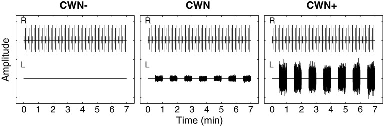
Schematic of the test condition (CWN, center panel) and control conditions (CWN− and CWN+, left and right panels, respectively). The click train delivered to the right ear is shown in the top half of each panel, and the noise delivered to the left ear is shown in the bottom half. The click train is the same for all conditions. For the sake of visual clarity, the number of clicks shown has been reduced by a factor of 200. In the CWN− control condition, no acoustic noise stimulus is presented to the left ear, as indicated by the flat horizontal line. In the CWN test condition and CWN+ control condition, acoustic noise is turned on and off in 30-s intervals.
Analysis
Detection of MEMR
Before considering MOC shifts, it is critical to establish whether any level differences observed might be influenced by the MEMR. MEMR activation reduces sound transmission through the middle ear primarily at low frequencies, with smaller effects at frequencies above 1 kHz (Møller 1962; Rabinowitz 1977). Activation of the MEMR has been shown to reduce OAE amplitudes (Whitehead et al. 1991). Many studies of MOC shifts using TEOAEs have therefore inferred the absence of MEMR activation by using noise levels that do not elicit the MEMR as assessed using standard clinical measurements employing a 226-Hz probe tone (e.g., Collet et al. 1990; De Boer and Thornton 2008; De Ceulaer et al. 2001). However, others have suggested that subclinical activation of the MEMR may be sufficient to impact measurement of MOC shifts (Feeney and Keefe 2001; Guinan et al. 2003), which would limit the usefulness of clinical measurement criteria. Sensitive nonclinical methods for MEMR detection have been described in the literature, for instance, using SFOAEs (Goodman and Keefe 2006; Guinan et al. 2003). In the present study, MEMR activation was detected using the TEOAE click stimulus as a probe.
If the sound pressure recordings of the click stimuli are time windowed around the clicks, they can be examined for level differences occurring when the noise is on versus off. The p1,2 (suppressor) click was time windowed starting 2 ms before the peak of the click and ending 2 ms after the peak of the click. The windowed clicks were then filtered using a 1/3-octave bandpass finite impulse response (FIR) filter centered at 1 kHz. Within this time window, the energy is expected to be dominated by stimulus energy because TEOAE energy around 1 kHz has a much longer expected round-trip travel delay (Tognola et al. 1997). A possible exception involves cases where strong synchronous spontaneous emissions are present. The effect of this was not specifically examined in the current study. If this did affect results, it would tend to make MEMR detection overly sensitive, erring on the conservative side.
After time windowing and filtering, the RMS amplitude of each filtered click was computed. The top row of Figure 2 shows examples of stimulus levels across time for three different subjects in the test and control conditions. Interleaving of contralateral noise off and on is shown by blue and red dots, respectively. These panels demonstrate that drifts in stimulus levels occur across time. These drifts ranged from tenths of a decibel up to 1 dB or more. Some authors have described interleaving the contralateral noise on and off to account for these systematic changes (e.g., De Boer and Thornton 2008; Guinan et al. 2003; Hood et al. 1996, 2003). However, if there is a systematic monotonic trend of increasing or decreasing stimulus/TEOAE levels across time, interleaving by itself may not adequately account for this trend because the state that was presented second will always be different, on average, than the one that came first. In this study, it was found that if slow drifts were not removed by de-trending, all subjects showed statistically significant differences in stimulus levels, even in the control condition (CWN−) in which the noise generator was disconnected from the earphone.
FIG. 2.

Detection of MEMR activation. An example is shown for the test condition (CWN, center columns) and control conditions (CWN− and CWN+, left and right columns, respectively). Each column shows data obtained from a different subject. Each colored dot in the top and middle rows represents a click stimulus level. Blue dots show levels obtained with contralateral noise off, and red dots show levels obtained with contralateral noise on. The top row shows stimulus levels across time. A trend line is shown on top of the dots in black. The middle row shows stimulus levels after de-trending and artifact rejection. The bottom row shows empirical distribution functions (edfs) for the resampled differences. The edfs are shown as thin solid lines and the 99 % confidence intervals are shown by thick solid lines. Mean differences from measured data are shown by green dashed lines. Mean differences that fall within the confidence intervals (CWN− and CWN, in this figure) indicate no significant difference and are interpreted as MEMR absent. Mean differences that fall outside the confidence intervals (CWN+, in this figure) indicate a significant difference and are interpreted as MEMR present.
Slow drifts can potentially be removed with de-trending techniques such as a running average, low-pass FIR filter, or polynomial fit. However, in this data set, it was not uncommon to see sudden changes in signal level (e.g., the top right panel in Fig. 2). In such cases, a median filter is more effective at removing edge discontinuities without smearing. Accordingly, a median filter (Little and Jones 2010) was used to find the trend line. The trend line was adjusted by setting the maximum value to 0 dB, after which the trend line was converted to linear units. The original waveforms were then divided by the corresponding values on the adjusted trend line. The result of this process was to hold the waveform with maximum amplitude constant and increase all other amplitudes so that the trend was removed. The choice of the number of samples over which the median was computed, determined empirically, was 41 samples, corresponding to 3.7 s (approximately 12 % of the length of the 30-s interleaving). The median fit was subsequently smoothed using a 20-point mean smoother to remove small, spurious discontinuities. This number of samples provided the minimum amount of de-trending required so that recordings in the control condition with the noise generator disconnected (CWN−) did not show a significant difference between conditions. Trend lines are shown in black in the top row of Figure 2. Artifact rejection was applied to discard waveforms contaminated by intermittent noise (Goodman et al. 2009). Finally, the first five recordings on either side of the interleaving between noise off and noise on were discarded. Examples of stimulus levels after de-trending and artifact rejection are shown in the middle row of Figure 2.
The presence of MEMR was determined by comparing the mean differences in de-trended stimulus levels between the noise on and off conditions for statistical significance. Significant differences in stimulus levels were expected to result from changes in middle ear impedance due to MEMR activation. A statistical resampling with replacement (bootstrap) algorithm (Efron and Tibshirani 1993) was implemented using custom software written in MATLAB (The MathWorks, Inc.). Recall that the dataset consisted of one set of n = 2,400 recordings with contralateral noise off and one set of n = 2,400 recordings with contralateral noise on. For this statistical test, each recording was bandpass filtered at 1 kHz and time windowed to a length of 4 ms as described previously. The null hypothesis was that there was no difference between the two sample sets. Under this hypothesis, all the samples were considered as a single pool of samples (N = 4,800 recordings). The distribution of differences taken from this single pool was found by randomly selecting (with replacement) two resampled sets of 2,400 recordings each. The 2,400 recordings in each resampled set were averaged. The RMS amplitude of each average was calculated, and the two RMS values were subtracted to yield a single difference amplitude. This resampling operation was repeated 10,000 times. The 10,000 differences were sorted to create a resampled empirical distribution function (edf). This distribution showed the expected differences from sampling under the null hypothesis (i.e., there was no difference between the two sample sets of with and without contralateral noise). Finally, the actual mean difference value obtained between the two sample sets was compared to the resampled edf. The actual mean difference was considered significant at the level of α = 0.01 if it fell outside the 0.005 or 0.995 points (99 % confidence intervals) on the resampled edf. Rejection of the null hypothesis was interpreted to mean that the two sample sets had different amplitudes, and that the difference was due to MEMR activation, given that slow drift artifacts had been removed prior to statistical analysis. The bottom row of Figure 2 shows the edfs describing the decibel differences between recordings in the noise on and off conditions. The left and middle panels show that the observed mean difference lies within the 99 % confidence intervals of the edfs, indicating no significant difference and therefore no evidence of MEMR activation. The right panel shows that the observed difference lies outside the 99 % confidence intervals and is therefore indicative of MEMR activation, which would be expected given the presence of high-level CWN.
In a statistical approach such as this, alpha levels must be chosen as criteria for determining significance. Alpha levels must be chosen for the test of MEMR detection, as well as for the test of MOCR detection (as described later). There is an interaction between these two alpha levels in terms of the total number of significant MOC shifts detected. For instance, if the alpha levels for both tests are made the same, then more conservative (smaller) alpha levels for MEMR detection will result in more subjects being considered for MOC shifts, but this effect will be offset by the stringent MOCR detection, which will result in fewer subjects being identified as having a significant shift. In contrast, a less conservative (larger) alpha level will result in more instances of MEMR being identified and fewer subjects being considered for MOC shifts; however, the laxer MOC shift criterion may result in more spurious shifts being identified as MOC shifts. These tradeoffs are further complicated by the fact that the signals being considered (click stimuli vs. TEOAEs) have vastly different signal-to-noise ratios (SNRs). Determining the optimal alpha levels was beyond the scope of this study, and results are reported for alpha levels of 0.01.
Detection of MOCR
TEOAE recordings were analyzed using a manner similar to the analysis of stimulus recordings described in the previous section. The portions of TEOAE waveforms prior to the peak of the stimulus were discarded, after which, 2-ms cosine-squared ramps were applied to the onsets and offsets. Eleven overlapping, 1/3-octave bandpass filters were created using a Hann window-based design method. Filter order decreased as center frequency and bandwidth increased. The filter center frequencies spanned 1–10 kHz, and the filter orders ranged from 2000 to 200, which corresponded to filter group delays of 10.4 to 2.0 ms, respectively. The group delays of the filters were subtracted from filtered waveforms to ensure correct temporal alignment after filtering.
For TEOAEs at each filter center frequency, an analysis time window was determined based on the 95 % confidence intervals for the expected SFOAE latencies in humans reported by Shera et al. (2002). Delay at each frequency was computed as
 |
1 |
where τSFOAE is round-trip SFOAE delay in millisecond, f is frequency in kilohertz, and values for β and α are given in Table I of Shera et al. (2002). These times were used under the assumption that TEOAEs and SFOAEs are generated by linear coherent reflection (Kalluri and Shera 2007; Shera and Guinan 1999) and should therefore have similar latencies. The confidence intervals reported by Shera et al. (2002) were widened by a factor of 1.25 to account for potential differences due to higher stimulus levels (Schairer et al. 2006). The amplitudes of TEOAE signals and noise floors within each analysis window were estimated using a two-buffer method (Kemp et al. 1990). Each bandpass-filtered waveform was put into one of two analysis buffers in an alternating fashion. The signal was estimated by adding the two buffers and dividing by two. The noise floor was estimated by subtracting the two buffers and dividing by two. The signal and noise floor were quantified by the RMS amplitude (decibel SPL).
Figure 3 shows an example of mean 1 kHz TEOAE waveforms obtained with the contralateral noise off (thicker blue lines) and on (thinner red lines). Differences between the tracings can be seen, with amplitudes generally being smaller with noise on (red tracings). However, it is not possible to determine from these plots if the differences are statistically significant. In order to assess the statistical significance of MOC shifts, the distributions of the sampling means of the differences in RMS TEOAE levels with the noise turned off and on were estimated using the resampling with replacement algorithm described previously. Prior to computing the algorithm, RMS amplitudes of the filtered waveforms were calculated within the analysis windows (Fig. 4, top row). Examination of TEOAE levels across time showed less apparent trends relative to those seen in the stimulus levels across time. This is likely due to the large difference in SNRs (note the difference in scale between the top panel of Figs. 2 and 4). However, the presence of drift in the stimulus levels suggests that drift was also present in the TEOAE levels across time. Because of the differences in SNR, it was found that using the same de-trending operation on the TEOAE levels as the stimulus levels introduced new trends in the TEOAE levels and was therefore not appropriate. For the TEOAE levels, a 167-point median filter was used (in contrast to a 41-point median filter for the stimulus levels), and the fit was smoothed with a 20-point mean filter. This procedure removed the underlying trends and did not introduce any new apparent trends. Examples of de-trended TEOAE levels are shown in the middle panel of Figure 4.
FIG. 3.
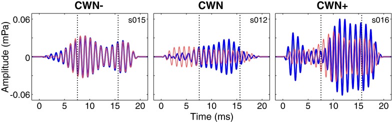
Mean TEOAE waveforms filtered at 1 kHz (11 filter center frequencies were examined in the current study, but only 1 kHz is shown here). Waveforms obtained with contralateral noise off and on are shown by thick blue and thinner red tracings, respectively. Time zero corresponds to the location of the click stimulus peak. Dotted vertical lines indicate the time range of the expected emissions (see text for details).
FIG. 4.

Detection of MOC shifts. Column layout is similar to that described in Figure 2 with regard to conditions and subjects. The top row shows TEOAE RMS amplitudes across time. Each colored dot represents the level of a filtered TEOAE waveform, with blue dots corresponding to contralateral noise off and red corresponding to contralateral noise on. A trend line is shown on top of the dots in black. The middle row shows RMS amplitudes after de-trending and artifact rejection. The bottom row shows empirical distribution functions (edfs) for the resampled differences. The edfs are shown as thin solid lines and the 99 % confidence intervals are shown by thick solid lines. Mean differences from measured data are shown by green dashed lines. Mean differences that fall within the confidence intervals (CWN−, in this figure) indicate no significant difference and are interpreted as a nonsignificant MOC shift. Mean differences that fall outside the confidence intervals (CWN and CWN+, in this figure) indicate a significant difference and may be interpreted as significant MOC shift. MOC shifts in the negative direction indicate that TEOAE amplitudes are smaller for the contralateral noise on than off.
After de-trending, edfs for the difference in RMS amplitudes of TEOAEs were obtained in the same manner as described for MEMR detection. An MOC shift was considered statistically significant when the observed difference in mean RMS amplitude between the noise on and off conditions fell outside the 0.005 and 0.995 points on the edf. Additionally, the MEMR was required to be absent in order for an MOC shift to be considered significant. If a significant difference was found between TEOAE levels but the MEMR was present, the result was considered inconclusive because the contribution of the MOCR could not be determined. Examples of edfs for determining significant MOC shifts are shown in the bottom panel of Figure 4.
Nonsignificant MOC shifts could be due to lack of MOCR. Alternatively, nonsignificant shifts could be due to poor SNR at a given frequency, making the results inconclusive. Within each analysis window, the presence or absence of TEOAE energy was determined by computing the mean SNRs. TEOAEs were considered present when the SNR was ≥6 dB. Recordings with SNR <6 dB were not statistically analyzed for MOC shifts.
RESULTS
Individual results
Figure 5 shows MOC shifts at all frequencies for the subset of subjects tested in the control conditions (CWN− and CWN+). MOC shifts are quantified as the decibel difference in RMS amplitude between TEOAEs obtained in the noise on and off conditions. Shifts in the negative direction indicate that TEOAE levels decreased in the presence of CWN. Shifts in which the MEMR was present are indicated by × markers. Even though MEMR was tested only at 1 kHz, if detected, the MEMR was considered a potential artifact at other frequencies, and therefore, all of that subject's MOC results were marked with an ×. For subjects participating in test and control conditions, MEMR was tested separately for each condition. As expected, in the CWN− condition (noise generator disconnected from the earphone), no MEMR activation was detected in any of the subjects (0/6), while in the CWN+ condition (high-level noise), MEMR activation was detected in all of the subjects (6/6).
FIG. 5.

Individual MOC shift results for the control conditions (CWN− on the left and CWN+ on the right). Each row shows results for a different frequency band. Within each row, the decibel difference between TEOAE recordings made with contralateral noise off and on is displayed. Negative values indicate a reduction in TEOAE level with contralateral noise on. Mean differences shown by × marks indicate subjects who had significant MEMR activation. Mean differences shown by circles indicate subjects who did not have significant MEMR activation. Filled red circles indicate significant MOC shifts, while open circles indicate nonsignificant MOC shifts. No markers are shown if TEOAE SNR was <6 dB at that frequency.
In Figure 5, MOC shifts occurring in the absence of MEMR activation are shown by circles. Significant MOC shifts (i.e., the mean difference in RMS amplitude falls outside the 99 % CIs of the resampled distributions) are shown as filled circles, while those that do not represent significant shifts are shown as open circles. No marker is shown if the TEOAE SNR was <6 dB. At the level of α = 0.01, a 1 % type I error rate (finding an MOC shift significant when it is not) is expected. In the CWN− condition, significant MOC shifts were seen only in subject 11 at 6.3 and 8.0 kHz. This represents an error of 3.2 % (2/63), which is not inconsistent with the small sample size examined in the current study. In contrast, it was expected that in the CWN+ condition, apparent MOC shifts would be seen often, especially at the lower frequencies where MEMR activation produces a strong effect. These shifts are presumably a mixture of MOCR and MEMR effects. No attempt was made in this study to disentangle the two effects. Rather, wherever MEMR activation occurred, the shifts were marked with an ×, as described above, so as to avoid misinterpretation.
Figure 6 shows MOC shifts for all individuals in the test condition (CWN presented at 30 dB SL). Shifts due to MEMR and MOCR are indicated with the markers as described above for Figure 5. Additionally, no markers are shown if the TEOAE SNR was <6 dB. Results obtained without and with de-trending are shown on the left and right, respectively, for each subject. MEMR activation was detected in 3/16 subjects (18.75 %). For the remaining subjects, significant shifts were seen primarily from 1.0 to 3.2 kHz, with fewer shifts seen at 4 kHz and above. The lack of significant MOC shifts above 4 kHz is likely due to low SNR, as discussed further at the end of the “Results” section.
FIG. 6.

Individual MOC shift results for the test condition (CWN). Each row shows results for a different frequency band. Within each row, the decibel difference between TEOAE recordings made with contralateral noise off and on is displayed. Mean differences shown by × marks indicate subjects who had significant MEMR activation. Mean differences shown by circles indicate subjects who did not have significant MEMR activation. Filled red circles indicate significant MOC shifts, while open circles indicate nonsignificant MOC shifts. No markers are shown if TEOAE SNR was <6 dB at that frequency. Vertical bars are used to demarcate results as boxes for each subject. Within each box, results obtained without de-trending are shown on the left and results obtained with de-trending are shown on the right.
In most cases, qualitatively similar results were obtained with and without de-trending (see Fig. 6). Across all 135 cases, there was a median absolute magnitude difference of 0.04 dB (mean = 0.10 dB). However, a wide range of differences were seen across frequencies and across individuals (0.0006–1.38 dB). Similar results were seen when considering only the subset of 68 cases in which a significant MOC shift was present (median = 0.06 dB, mean = 0.11 dB, range = 0.001–0.71 dB). De-trending resulted in a smaller shift in over half of all cases (69 %, 93/135). In 4 % (6/135) of cases, de-trending changed whether the MOC shift was significant. In five of these six cases, de-trending resulted in a significant shift. However, these are too few cases to make a generalization regarding whether de-trending generally increases or decreases the number of significant shifts seen. It appears for the majority of subjects, de-trending does not affect the ability to detect an MOC shift, making de-trending less of a concern when examining group data. However, when considering individual subjects, de-trending of TEOAE data appears warranted. Subsequent results are reported for de-trended data only.
Group results
Figure 7 shows data grouped by frequency for the CWN condition only. Data at each frequency include only those subjects with present emissions and no MEMR activation. Mean MOC shifts (top panel) show strong frequency dependence. At frequencies below 4 kHz, a majority of subjects without MEMR had significant MOC shifts (62–85 %). At 4 kHz, 5/13 (38 %) subjects had significant MOC shifts, and at the higher frequencies, the number of shifts was even smaller (8–23 %). The top panel of Figure 7 also shows that the directions of significant MOC shifts were almost always in the negative direction (65/68, 96 %), meaning that turning on the contralateral noise decreased TEOAE amplitudes, as expected.
FIG. 7.

Group MOC shift results as a function of frequency. Results are shown for the test condition (CWN) only. Top panel shows mean MOC shifts in decibel. Negative values indicate a reduction in TEOAE amplitude with contralateral noise on. Data representing statistically significant shifts are shown by filled red circles encompassed by white bars. Data representing nonsignificant shifts are shown by open circles encompassed by black bars. Bottom panel shows the magnitude of minimum detectable shifts in decibel. These values were obtained as the absolute value of the lower 99 % confidence interval of the resampled distributions. Significant and nonsignificant shifts are represented as described in the top panel.
MOC shift results were similar from 1.0 to 3.2 kHz, so group results were collapsed across this frequency range to examine overall trends in the data. The absolute magnitudes of MOC shifts had a median of 1.94 dB (range = 0.34–6.51 dB) and nonsignificant shifts had a median of 0.49 dB (range = 0.01–2.51 dB). In general, there was an overlap between the distributions of significant and nonsignificant mean shifts. Although absolute shifts larger than 2.51 dB were always significant, shifts of this magnitude accounted for only 20/57 (35 %) of significant shifts from 1.0 to 3.2 kHz. This suggests that using a simple shift magnitude cutoff value would not reliably distinguish significant from nonsignificant shifts.
It was of interest to examine the number of frequency bands at which each individual subject showed significant MOC shifts. This examination was restricted to the six frequency bands from 1.0 to 3.2 kHz because few subjects had significant MOC shifts in higher bands. In a given individual, the number of bands which showed a significant MOC shift ranged from 2 to 6, with a median of 5 (see Fig. 6). Only 3/13 (23 %) subjects had significant shifts in all six frequency bands.
The bottom panel of Figure 7 shows the smallest magnitudes of significant MOC shifts that were detectable using the methods described in this paper. This value was obtained as the absolute value of the lower 99 % confidence interval of the resampled distribution. The size of minimum detectable shifts demonstrated a large amount of individual variability. When collapsed across 1.0–3.2 kHz, minimum detectable shifts had a median value of 0.91 dB (range = 0.10–3.25 dB). There was no apparent difference between minimum detectable shifts associated with significant and nonsignificant MOC shifts. These data indicate that in some cases, very small shifts (tenths of a dB) can reach statistical significance.
Much of the variability in minimum detectable shift magnitudes was attributable to SNR, with higher SNR resulting in a smaller minimum detectable shift. Figure 8 shows a scatter plot of minimum detectable shifts as a function of SNR. Data from all frequencies (1.0–10.0 kHz) are included. To improve visualization, shifts at low frequencies (1.0–3.2 kHz) are shown as circles, and shifts at high frequencies (4.0–10.0 kHz) are shown as triangles. Minimum detectable shifts associated with significant and nonsignificant shifts are shown as filled red and unfilled markers, respectively. The solid black line is a robust bisquare-weighted fit of the form y = aebx, where a = 6.11 and b = −0.08. Dashed lines indicate the 99 % confidence intervals of the fit. Minimum detectable shifts decreased in magnitude with increasing SNR. The R2 value of the fit was 0.85, indicating that 85 % of the variance in minimum detectable shifts is explained by SNR. Frequencies below 4 kHz tended to have lower minimum detectable shifts presumably because they were associated with higher SNRs. Frequencies at 4 kHz and above had lower SNRs and higher minimum detectable shifts. This may explain why there were many nonsignificant MOC shifts at high frequencies. While a 6-dB SNR is generally considered adequate to detect the presence of TEOAEs, from Figure 8, it is clear that much higher SNRs (18–30 dB) are required to detect the magnitudes of MOC shifts that are typically seen (~2 dB, see Fig. 7, top panel).
FIG. 8.

Minimum detectable shift as a function of SNR. Data are shown for all frequencies and are grouped by low frequencies (<4 kHz, shown as circles) and high frequencies (≥4 kHz, shown as triangles). Statistically significant shifts (p < 0.01) are shown as filled red markers. Nonsignificant shifts are shown as unfilled markers. The solid black line is a robust exponential fit to the data of the form y = ae bx, where a = 6.11 and b = −0.08. Dashed lines indicate 99 % confidence intervals of the fit. R 2 value of the fit was 0.85.
DISCUSSION
Detecting significant MOCR shifts in individuals may have clinical applications, such as predicting susceptibility to noise-induced hearing loss and providing insight into difficulty hearing in noise. This paper demonstrates a method of detecting such shifts in individual subjects. Further research is needed to establish whether such an approach can provide clinically useful information. Future studies should consider the following technical issues when measuring MOC shifts.
Stimulus levels
The current study did not explore optimal presentation levels, either for TEOAE stimuli or for MOCR activators. Optimal levels involve interactions between click levels and CWN levels, as well as the stimulus bandwidth, extraction paradigm, and presentation rate, so levels cannot be chosen in isolation. This is a large parameter space, and further research is needed to determine the optimal combination. However, based on the results of the current study, a recommended starting place is to present TEOAE stimuli at 30 dB SL using a linear extraction paradigm and CWN at 30 dB SL. These suggestions are discussed in more detail below.
With regards to CWN levels, the current study used a fixed sensation level. One disadvantage of the fixed level approach is that it does not allow measurement of MOC shifts in a percentage of subjects with low MEMR activation thresholds. An alternative approach would be to optimize CWN levels for each subject. Individual optimization would use the highest activator level that did not activate the MEMR, presumably maximizing the measured MOC shift. However, the fixed level approach may be preferred because it allows for a comparison of MOC shifts across subjects that are less influenced by individual variability in MEMR sensitivity. It is unclear whether individually optimized or fixed MOC activator levels, or some combination of the two, would prove most clinically useful, and further research is needed in this area.
Regardless of which approach is used, the current results suggest that it is important to employ a sensitive MEMR test in each individual. Some previous studies have inferred lack of MEMR activation based on clinical immittance measurements (e.g., Collet et al. 1990; De Boer and Thornton 2008; De Ceulaer et al. 2001). However, it is possible that subclinical activation of the MEMR could confound or contaminate MOC shifts (Feeney and Keefe 2001; Guinan et al. 2003). Some studies have reported monitoring of MEMR activation using techniques that may be more sensitive than standard clinical measurements (Guinan et al. 2003; Goodman and Keefe 2006). Contralateral white noise levels used in current study (30 dB SL) were chosen based on previous reports (e.g., Hood et al. 1996), and it was found that 3 out of 16 subjects (19 %) had evidence of MEMR activation. Without careful MEMR detection methods, the shifts seen in these subjects may have been incorrectly attributed to MOCR activation.
Frequency range
Physiologic data in animals indicate that MOC innervation is densest in the mid-frequency region of the cochlea, though comparable data in humans are currently lacking (Guinan 2006). Previous MOC studies using TEOAEs in humans have shown the largest MOC shifts in the 1–4-kHz range (e.g., Berlin et al. 1993; Collet et al. 1990). However, few studies have measured TEOAEs at frequencies above 6 kHz (Goodman et al. 2009; Keefe et al. 2011), and these studies did not examine MOC shifts. The current study examined MOC shifts that included high frequencies by using TEOAE stimuli with a bandwidth extending to 10 kHz and a nonlinear extraction paradigm. Consistent with previous studies, the region below 4 kHz showed the most MOC shifts. Few MOC shifts were seen at higher frequencies.
Based on the current results, it appears that the lack of MOC shifts above 4 kHz is due to a weak MOCR effect on TEOAEs at high frequencies and/or the inability to detect MOC shifts because of poorer SNR. Because TEOAE SNRs in the current study were generally not sufficient at frequencies >4 kHz (see Fig. 8), it could not be determined whether MOCR effects were present at high frequencies. The lower SNRs at higher frequencies were due to a combination of higher noise floors and lower emission levels. The lower emission levels may have been cochlear in origin and/or due to middle ear transfer function. Measurement of MOCR effects at higher frequencies requires the use of a nonlinear paradigm due to the short cochlear delays of high-frequency TEOAEs (Goodman et al. 2009). In addition, longer averaging times would be needed to achieve sufficient SNRs at higher frequencies, and this might be an issue in terms of clinical feasibility. Further study is needed to answer the question of MOCR effects on high-frequency TEOAEs.
Future research into clinical applications of MOCR using TEOAEs may benefit from concentrating on frequencies ≤4 kHz because the longer latencies and higher SNRs of TEOAEs at these frequencies allow for more efficient measurement paradigms. Detection of MOCR effects at lower frequencies would most likely be optimized using a linear extraction paradigm. Compared to the double-evoked nonlinear paradigm used in the current study, a linear paradigm is significantly faster, obtaining the same number of averages in 1/3 of the time. In addition, a linear paradigm retains the entire emission, whereas the nonlinear method cancels the linear portion of the emission, potentially discarding information about MOC shifts. Finally, the use of a higher level suppressor stimulus in the nonlinear method likely partially activates the MOCR, which would reduce the size of measured MOC shifts (Guinan et al. 2003). It may also be possible to use a simple subtraction of the recordings made with and without contralateral noise to cancel stimulus artifact at high frequencies. Such a technique would presumably be more sensitive to MOC shifts than the double-evoked nonlinear paradigm used in this study. However, drift artifact is potentially still a problem because without perfect de-trending, the subtraction will leave small residual stimulus artifact that will overlap in time with high-frequency TEOAEs.
Averaging
The current study used a fixed number of recorded averages for all subjects. A more efficient measurement paradigm could adaptively change the number of recorded averages based on TEOAE SNR and the desired minimum detectable shift. For example, if the ability to detect MOC shifts of ≥1 dB was desired, an SNR of approximately 30 dB would be targeted (see Fig. 8). This SNR would be targeted at all frequencies of interest. One of the particular challenges of TEOAEs is that all the frequencies are measured at once, but the SNRs vary across frequency. Therefore, the number of averages needed would be dictated by the frequencies having the worst SNR. Averaging would continue until a certain percentage of frequencies met the target SNR or until a maximum number of averages was obtained.
Drift control
Interleaving noise and no-noise conditions are an important control for drift when performing MOC studies. In general, faster interleaving rates would provide a better drift control. However, there are limits on the rate of interleaving due to time constants associated with the onset and offset of MOCR (Backus and Guinan 2006). In the current study, an interleaving rate of 30 s was chosen. While this rate appears to have been adequate, it is possible that a somewhat faster interleave rate, such as 15 s, may provide better drift control.
Many previous studies of MOCR effects have not carefully controlled for slow drift. Some studies have used interleaving of noise on and noise off states to account for relatively slow changes across time (e.g., De Boer and Thornton 2008; Guinan et al. 2003; Hood et al. 1996, 2003). In the current study, interleaving by itself did not always provide adequate protection from contamination by slow drifts. Drifts have the potential to make MOC shifts more or less significant, depending on the direction of change. While these effects may cancel each other in group data, de-trending should not be omitted when determining MOC shifts in individuals.
MOCR frequency effects
Based on the results of this study, it appears that some normal-hearing subjects will show significant MOC shifts at some frequencies but not at others, even when there is an adequate SNR to permit detection (see for example, Fig. 6, subject 1 from 1.0 to 3.2 kHz). This is in agreement with previous work. In their study examining individual MOC shifts using SFOAEs, Backus and Guinan (2007) found that in a given individual, MOC shifts were sometimes present at a given frequency but absent at other nearby frequencies. In the current study, TEOAEs were analyzed in 11 1/3-octave frequency bands. No overall pattern was observed which would indicate weaker MOCR activation in any particular frequency region. This suggests that individual variability across frequency may be a common result. TEOAEs provide an efficient way to examine these individual patterns of MOC activation across frequency. Future studies may provide insight into the sources of this variability as well as the stability over time.
CONCLUSIONS
In individual subjects, MOC shifts quantified by changes in TEOAE amplitude can be examined for statistical significance using a resampling approach. Careful control of confounds (slow amplitude drifts and MEMR activation) is important to ensure accurate results. The magnitude of minimum detectable shifts is dependent on TEOAE SNR, making it important to obtain an adequate number of averages to attain high SNRs. In the current study, 50 % of detected MOC shifts had magnitudes between 1.1 and 2.9 dB. On average, detection of shifts of these magnitudes required SNRs of approximately 9–22 dB. Few shifts were seen at frequencies ≥4 kHz; however, the ability to measure shifts in this frequency range was limited by poor SNRs. Overlap was found in the magnitudes of MOC shifts that were significant and nonsignificant. This suggests that determining the presence of MOC shifts in an individual should be based on individualized resampling rather than using minimum shift criteria obtained from group data.
ACKNOWLEDGMENTS
The authors thank the two anonymous reviewers for their helpful comments regarding the manuscript. This work was supported by a 2010 Student Research Grant in Audiology and a 2010 Clinical Research Grant from the American Speech-Language-Hearing Foundation.
Contributor Information
Shawn S. Goodman, Phone: +1-319-3358761, FAX: 1-319-3358851, Email: shawn-goodman@uiowa.edu
Ian B. Mertes, Email: ian-mertes@uiowa.edu
James D. Lewis, Email: james-lewis@uiowa.edu
Diana K. Weissbeck, Email: diana.weissbeck@huskers.unl.edu
REFERENCES
- Backus BC. Bias due to noise in otoacoustic emission measurements. J Acoust Soc Am. 2007;121:1588–1603. doi: 10.1121/1.2434831. [DOI] [PubMed] [Google Scholar]
- Backus BC, Guinan JJ., Jr Time-course of the human medial olivocochlear reflex. J Acoust Soc Am. 2006;119:2889–2904. doi: 10.1121/1.2169918. [DOI] [PubMed] [Google Scholar]
- Backus BC, Guinan JJ., Jr Measurement of the distribution of medial olivocochlear acoustic reflex strengths across normal-hearing individuals via otoacoustic emissions. J Assoc Res Otolaryngol. 2007;8:484–496. doi: 10.1007/s10162-007-0100-0. [DOI] [PMC free article] [PubMed] [Google Scholar]
- Berlin CI, Hood LJ, Wen H, Szabo P, Cecola RP, Rigby P, Jackson DF. Contralateral suppression of non-linear click-evoked otoacoustic emissions. Hear Res. 1993;71:1–11. doi: 10.1016/0378-5955(93)90015-S. [DOI] [PubMed] [Google Scholar]
- Clarke EM, Ahmmed A, Parker D, Adams C. Contralateral suppression of otoacoustic emissions in children with specific language impairment. Ear Hear. 2006;27:153–160. doi: 10.1097/01.aud.0000204311.73871.41. [DOI] [PubMed] [Google Scholar]
- Collet L, Kemp DT, Veuillet E, Duclaux R, Moulin A, Morgon A. Effect of contralateral auditory stimuli on active cochlear micro-mechanical properties in human subjects. Hear Res. 1990;43:251–261. doi: 10.1016/0378-5955(90)90232-E. [DOI] [PubMed] [Google Scholar]
- Dallos P. The active cochlea. J Neurosci. 1992;12:4575–4585. doi: 10.1523/JNEUROSCI.12-12-04575.1992. [DOI] [PMC free article] [PubMed] [Google Scholar]
- De Boer J, Thornton ARD. Neural correlates of perceptual learning in the auditory brainstem: efferent activity predicts and reflects improvement at a speech-in-noise discrimination task. J Neurosci. 2008;28:4929–4937. doi: 10.1523/JNEUROSCI.0902-08.2008. [DOI] [PMC free article] [PubMed] [Google Scholar]
- De Ceulaer G, Yperman M, Daemers K, Van Driessche K, Somers T, Offeciers FE, Govaerts PJ. Contralateral suppression of transient evoked otoacoustic emissions: normative data for a clinical test set-up. Otol Neurotol. 2001;22:350–355. doi: 10.1097/00129492-200105000-00013. [DOI] [PubMed] [Google Scholar]
- Efron B, Tibshirani RJ. An introduction to the bootstrap. New York: Chapman and Hall; 1993. [Google Scholar]
- Feeney MP, Keefe DH. Estimating the acoustic reflex threshold from wideband measures of reflectance, admittance, and power. Ear Hear. 2001;22:316–332. doi: 10.1097/00003446-200108000-00006. [DOI] [PubMed] [Google Scholar]
- Garinis AC, Glattke T, Cone-Wesson BK. TEOAE suppression in adults with learning disabilities. Int J Audiol. 2008;47:607–614. doi: 10.1080/14992020802129402. [DOI] [PubMed] [Google Scholar]
- Goodman SS, Keefe DH. Simultaneous measurement of noise-activated middle-ear muscle reflex and stimulus frequency otoacoustic emissions. J Assoc Res Otolaryngol. 2006;7:125–139. doi: 10.1007/s10162-006-0028-9. [DOI] [PMC free article] [PubMed] [Google Scholar]
- Goodman SS, Fitzpatrick DF, Ellison JC, Jesteadt W, Keefe DH. High-frequency click-evoked otoacoustic emissions and behavioral thresholds in humans. J Acoust Soc Am. 2009;125:1014–1032. doi: 10.1121/1.3056566. [DOI] [PMC free article] [PubMed] [Google Scholar]
- Guinan JJ., Jr . The physiology of olivocochlear efferents. In: Dallos PJ, Popper AN, Fay RR, editors. The cochlea. New York: Springer; 1996. pp. 435–502. [Google Scholar]
- Guinan JJ., Jr Olivocochlear efferents: anatomy, physiology, function and the measurements of efferent effects in humans. Ear Hear. 2006;27:589–607. doi: 10.1097/01.aud.0000240507.83072.e7. [DOI] [PubMed] [Google Scholar]
- Guinan JJ, Jr, Backus BC, Lilaonitkul W, Aharonson V. Medial olivochochlear efferent reflex in humans: otoacoustic emission (OAE) measurement issues and the advantages of stimulus frequency OAEs. J Assoc Res Otolaryngol. 2003;4:521–540. doi: 10.1007/s10162-002-3037-3. [DOI] [PMC free article] [PubMed] [Google Scholar]
- Hood LJ, Berlin CI, Hurley A, Cecola RP, Bell B. Contralateral suppression of transient-evoked otoacoustic emissions in humans: intensity effects. Hear Res. 1996;101:113–118. doi: 10.1016/S0378-5955(96)00138-4. [DOI] [PubMed] [Google Scholar]
- Hood LJ, Berlin CI, Bordelon J, Rose K. Patients with auditory neuropathy/dys-synchrony lack efferent suppression of transient evoked otoacoustic emissions. J Am Acad Audiol. 2003;14:302–313. [PubMed] [Google Scholar]
- Kalluri R, Shera CA. Near equivalence of human click-evoked and stimulus-frequency otoacoustic emissions. J Acoust Soc Am. 2007;121:2097–2110. doi: 10.1121/1.2435981. [DOI] [PubMed] [Google Scholar]
- Keefe DH. Double-evoked otoacoustic emissions. I. Measurement theory and nonlinear coherence. J Acoust Soc Am. 1998;103:489–3498. doi: 10.1121/1.423058. [DOI] [PubMed] [Google Scholar]
- Keefe DH, Goodman SS, Ellison JC, Fitzpatrick DF, Gorga MP. Detecting high-frequency hearing loss with click-evoked otoacoustic emissions. J Acoust Soc Am. 2011;129:245–261. doi: 10.1121/1.3514527. [DOI] [PMC free article] [PubMed] [Google Scholar]
- Kemp DT, Ryan S, Bray P (1990) A guide to the effective use of otoacoustic emissions. Ear Hear 11:93-105 [DOI] [PubMed]
- Little MA, Jones NS (2010) Sparse Bayesian step-filtering for high-throughput analysis of molecular machine dynamics. Proc IEEE Int Conf Acoust Speech Signal Process, pp. 4162-4165
- Maison SF, Liberman MC. Predicting vulnerability to acoustic injury with a noninvasive assay of olivocochlear reflex strength. J Neurosci. 2000;20:4701–4707. doi: 10.1523/JNEUROSCI.20-12-04701.2000. [DOI] [PMC free article] [PubMed] [Google Scholar]
- Micheyl C, Collet L. Involvement of the olivocochlear bundle in the detection of tones in noise. J Acoust Soc Am. 1996;99:1604–1610. doi: 10.1121/1.414734. [DOI] [PubMed] [Google Scholar]
- Møller A. Acoustic reflex in man. J Acoust Soc Am. 1962;34:1524–1534. doi: 10.1121/1.1918384. [DOI] [Google Scholar]
- Muchnik C, Ari-Evan Roth D, Othman-Jebara R, Putter-Katz H, Shabtai EL, Hildesheimer M. Reduced medial olivocochlear bundle system function in children with auditory processing disorders. Audiol Neurootol. 2004;9:107–114. doi: 10.1159/000076001. [DOI] [PubMed] [Google Scholar]
- Rabinowitz (1977) Acoustic-reflex effects on the input admittance and transfer characteristic of the human middle-ear. Dissertation, Massachusetts Institute of Technology
- Schairer KS, Ellison JC, Fitzpatrick D, Keefe DH. Use of stimulus-frequency otoacoustic emission latency and level to investigate cochlear mechanics in human ears. J Acoust Soc Am. 2006;120:901–914. doi: 10.1121/1.2214147. [DOI] [PMC free article] [PubMed] [Google Scholar]
- Shera CA, Guinan JJ., Jr Evoked otoacoustic emissions arise by two fundamentally different mechanisms: a taxonomy for mammalian OAEs. J Acoust Soc Am. 1999;105:782–798. doi: 10.1121/1.426948. [DOI] [PubMed] [Google Scholar]
- Shera CA, Guinan JJ, Jr, Oxenham AJ. Revised estimates of human cochlear tuning from otoacoustic and behavioral measurements. Proc Natl Acad Sci USA. 2002;99:3318–3323. doi: 10.1073/pnas.032675099. [DOI] [PMC free article] [PubMed] [Google Scholar]
- Tognola G, Grandori F, Ravazzani P. Time-frequency distributions of click-evoked otoacoustic emissions. Hear Res. 1997;106:112–122. doi: 10.1016/S0378-5955(97)00007-5. [DOI] [PubMed] [Google Scholar]
- Veuillet E, Collet L, Duclaux R. Effect of contralateral acoustic stimulation on active cochlear micromechanical properties in human subjects: dependence on stimulus variables. J Neurophysiol. 1991;65:724–735. doi: 10.1152/jn.1991.65.3.724. [DOI] [PubMed] [Google Scholar]
- Whitehead ML, Martin GK, Lonsbury-Martin BL. Effects of the crossed acoustic reflex on distortion-product otoacoustic emissions in awake rabbits. Hear Res. 1991;51:55–72. doi: 10.1016/0378-5955(91)90007-V. [DOI] [PubMed] [Google Scholar]