Accuracy and response-time distributions for decision-making: linear perfect integrators versus nonlinear attractor-based neural circuits

Abstract

Animals choose actions based on imperfect, ambiguous data. “Noise” inherent in neural processing adds further variability to this already-noisy input signal. Mathematical analysis has suggested that the optimal apparatus (in terms of the speed/accuracy trade-off) for reaching decisions about such noisy inputs is perfect accumulation of the inputs by a temporal integrator. Thus, most highly cited models of neural circuitry underlying decision-making have been instantiations of a perfect integrator. Here, in accordance with a growing mathematical and empirical literature, we describe circumstances in which perfect integration is rendered suboptimal. In particular we highlight the impact of three biological constraints: (1) significant noise arising within the decision-making circuitry itself; (2) bounding of integration by maximal neural firing rates; and (3) time limitations on making a decision. Under conditions (1) and (2), an attractor system with stable attractor states can easily best an integrator when accuracy is more important than speed. Moreover, under conditions in which such stable attractor networks do not best the perfect integrator, a system with unstable initial states can do so if readout of the system’s final state is imperfect. Ubiquitously, an attractor system with a nonselective time-dependent input current is both more accurate and more robust to imprecise tuning of parameters than an integrator with such input. Given that neural responses that switch stochastically between discrete states can “masquerade” as integration in single-neuron and trial-averaged data, our results suggest that such networks should be considered as plausible alternatives to the integrator model.

Introduction

The making of timely choices based on ambiguous, impoverished stimulus information is a basic part of survival and success for all living things. The acquisition, processing and filtering of such information by sensory transduction organs and multiple central nervous system relays adds noise to an already noisy fragment of data. Thus, our ability to produce appropriate behavioral responses in choice situations is even more impressive than it might naïvely seem.

The dynamics of such decision-making processes has been studied primarily during perceptual decision-making via two-alternative forced choice tasks (Shadlen and Newsome 1996; Ratcliff and Rouder 1998; Platt and Glimcher 1999; Glimcher 2001; Gold and Shadlen 2001; Shadlen and Newsome 2001; Usher and McClelland 2001; Roitman and Shadlen 2002; Romo et al. 2002; Glimcher 2003; Romo et al. 2004; Smith and Ratcliff 2004; Huk and Shadlen 2005; Luna et al. 2005; Gold and Shadlen 2007; Ratcliff 2008; Stanford et al. 2010; Yoshida and Katz 2011). In such tasks, a subject makes one of two distinctive responses depending on which stimulus is present (or, alternatively, depending on which is the dominant stimulus in a mixture); performance is evaluated in terms of overall accuracy for a given response speed (or range of speeds).

These tasks have been the source of a wealth of models, each based either on simulations of neural activity (Wang 2002; Wong and Wang 2006; Wong et al. 2007; Beck et al. 2008) or on the mathematical analysis of diffusion in an effective potential (Ratcliff 1978; Zhang et al. 2009; Zhou et al. 2009; Zhang and Bogacz 2010), which can be derived from models of neural activity (Usher and McClelland 2001; Smith and Ratcliff 2004; Bogacz et al. 2006; Sakai et al. 2006; Roxin and Ledberg 2008; Eckhoff et al. 2011). Regardless of their bases, decision-making models are typically judged according to two distinct criteria. First, how good—or, as it is often stated, how close to optimal—is the model at producing correct responses in a timely manner, given limited evidence and noise in the system? Second, how well does the model reproduce key behavioral (Feng et al. 2009) and electrophysiological (Wang 2001; Ditterich 2006) results beyond the inevitable increase in accuracy with either increased stimulus presentation time or with increased difference between stimulus representations, which arises naturally in all models?

Signal detection theory tells us that perfect integration of the difference in evidence for two alternatives is the optimal method for choosing between these alternatives (Wald 1947; Wald and Wolfowitz 1948). A corollary of this result to which many neuroscientists ascribe is that perfect integration is therefore also the optimal framework in which to study the neural basis of decision-making (Gold and Shadlen 2007). That is, integrators, typically implemented as drift diffusion models with fixed thresholds (Ratcliff 1978), are thought to provide both the most optimal models of decision making, and to best reproduce the basic behavioral (Ratcliff and McKoon 2008) and neural data, the latter of which suggest accumulation of information across time, at least when spiking is averaged across trials (Roitman and Shadlen 2002; Ratcliff et al. 2003). Moreover, biologically realistic circuits of neurons can approximate such integrators (Wang 2002), further supporting the conclusion that they are the appropriate model type to explain decision making in the nervous system.

There remain reasons to question this conclusion, however. First, the proof of optimality implicitly assumes either unbounded integration or unlimited time for a response. It is less clear whether an integrator is still favored once biologically plausible constraints (Bertsekas 2005; Frazier and Yu 2007; Cisek et al. 2009; Nigoyi and Wong-Lin 2010; Zhang and Bogacz 2010; Eckhoff et al. 2011; Standage et al. 2011) enforce a timely readout of activity in the decision-making circuit. Even with perfect readout of the final state of the system, the perfect integrator may not be optimal if firing rates and response times are limited (Zhang and Bogacz 2010). Finally, any neural implementation of a perfect integrator requires both the precise tuning of connection strengths and low within-circuit noise (Seung 1996; Usher and McClelland 2001; Wang 2002; Miller et al. 2003; Eckhoff et al. 2009), such that more naturalistic conditions might again favor robust approximations to an integrator based on multiple discrete attractors (Koulakov et al. 2002; Goldman et al. 2003), for which performance can be enhanced by additional noise (Deco et al. 2009; Miller and Katz 2010; Deco et al. 2013).

Furthermore, some of the extant behavioral data actually favor non-integrator models over perfect integrators. While most models reproduce the positive skewness of response times (a longer tail in the distribution for slow response times) (Ratcliff and Rouder 1998; Usher and McClelland 2001; Wong and Wang 2006), if bias and starting conditions are fixed, only nonlinear models reproduce the oft-observed phenomenon of slower responses on error trials than correct trials (Ditterich 2006; Wong and Wang 2006; Broderick et al. 2009). Perfect integrators must implement two separate mechanisms to produce slow and fast error responses: the former are produced by trial-to-trial variability in stimulus strength, while the latter are produced by trial-to-trial variability in the initial state of the system (Ratcliff and Rouder 1998).

Relatedly, the fit between the extant electrophysiological data and the predictions of an integrator model may not be as strong as once thought. Specifically, it has recently become clear that apparent ramps in neural activity can in some circumstances be artifactual results of across-trial averaging. Hidden-Markov model analyses of multi-unit neural activity (Jones et al. 2007), for instance, suggest that in some systems neural activity jumps between discrete states (Seidemann et al. 1996; Deco and Rolls 2006; Deco and Marti 2007; Okamoto et al. 2007; Eckhoff et al. 2009; Eckhoff et al. 2011; Ponce-Alvarez et al. 2012) but see (Bollimunta et al. 2012) with timing that varies from trial to trial. In such situations, the standard procedure of averaging across trials aligned to stimulus onset obscures the inherent structure of the system, forcing the emergence of an apparent ramp (Marti et al. 2008; Miller and Katz 2011). Without multi-neuronal data, such discrete jumps in activity are particularly difficult to recognize (but see (Okamoto et al. 2007)) or disprove, and thus it is as of yet unclear whether the activity of classically-defined decision-making neural ensembles have such structure.

Here we investigate conditions under which an attractor-based neural circuit, whose dynamics is most naturally described as jumps between discrete states (Deco et al. 2009; Miller and Katz 2010), could produce more accurate decisions than a perfectly linear integrating circuit. We have previously demonstrated that a multi-state attractor network built to reproduce such “jumpy” single-trial responses can out-perform (in terms of percent correct identification of appropriate taste-related behavior) the same network set to perform integration (Miller and Katz 2010). Here we present a more complete, rigorous comparison of perfect integrator and discrete attractor-based models.

We begin with the introduction of a simple time limit (a feature of many, if not most, sensorimotor decisions); we chose to begin with this constraint in order to put the perfect integrator in the best position—a model is less likely to reach the decision threshold in a finite time (we refer to the model as being “undecided” in such trials) when that system’s initial state is a stable attractor than when it is smoothly integrating. We then assess a range of methods for resolving such “undecided” trials, including the minimally accurate method (“guessing”) whereby 50 % of the trials that do not reach threshold are treated as correct, and a perfect mathematical readout whereby the sign of the decision variable determines the response, irrespective of the threshold. In between these extremes, we assess several biologically realistic mechanisms for reducing or eliminating undecided trials, each of which (see Methods for detailed descriptions) consists of either abruptly (“forcing a response”) or smoothly (an “urgency-gating signal”) pushing the system in the direction of the sign of the decision variable.

After describing a large number of simulations, the vast majority of which demonstrate limitations of the integrator model, we proceed to: 1) briefly explain how these results are consistent with previous work; and to 2) more closely examine extant behavioral and electrophysical data in relation to the models.

The sort of urgency-gating signal used in our simulations, which behavioral (Cisek et al. 2009) and electrophysiological data (Ditterich 2006; Churchland et al. 2008; Broderick et al. 2009) suggest arises during decision-making, speeds the likelihood of a response as time passes, as a reflection of the increasing cost of time spent accumulating information without acting upon a decision (Drugowitsch et al. 2012). We incorporate three methods for producing such an urgency-gating signal; specifically, we compare the implementation used by Cisek et al. (2009) to explain the relative lack of importance or weighting of early evidence compared to late evidence—a temporally ramping multiplicative factor (i.e. gain modulation) applied to the inputs to the decision-making system (see also (Ditterich 2006; Eckhoff et al. 2009; Nigoyi and Wong-Lin 2010; Eckhoff et al. 2011; Standage et al. 2011))—with both a ramping additive input current to the system and ramping decreases in the decision threshold (Bertsekas 2005; Frazier and Yu 2007). Each such signal is stimulus-nonspecific and could be produced by slow decay or rise in concentration of a neuromodulator such as norepinephrine (Shea-Brown et al. 2008), so is distinct from an integrator or accumulator.

Our formalism is a greatly simplified description of the dynamics of true neural circuitry, but it is complex enough that we cannot produce a single formula to fit to quantities such as a reaction time distribution. Other models do produce such analytic formulae, which gives them the benefit that parameters—such as level of noise, or threshold for response—can be adjusted with relative ease to produce best fits to experimental data.(Ratcliff et al. 2003; Eckhoff et al. 2008; Roxin and Ledberg 2008; Feng et al. 2009). Nevertheless, use of now-standard optimization routines with repeated calculations of probability distributions render trivial the fitting of parameters to data for more complicated models such as ours.

Within this formalism, we are able to compare multiple models of decision-making under a range of conditions, adjusting a single nonlinearity parameter to contrast perfect integrators (i. e., models with a nonlinearity of zero in our formalism), such as the drift diffusion model, with nonlinear, attractor-based models—two types of models that both reproduce an impressive range of behavioral and electrophysiological results. We analyze the decision-making accuracy of each model and assess a number of mechanisms that could improve accuracy, in the context of sensitivity to their biological plausibility. Moreover, we measure robustness of the results to imperfect tuning of parameters of the sort that almost certainly arises when the model is implemented within the brain’s neural circuitry. These analyses demonstrate that under many realistic conditions, nonlinear circuits that are not perfect integrators produce more accurate and more robust decision-making than the perfect integrator—a conclusion that, while suggested before, has not been tested in such a parametric manner previously.

Materials and methods

Our results are based on the temporal dynamics of the probability distribution of neural firing rates in a bounded system with fixed thresholds (Kiani et al. 2008). The probability distribution evolves following a deterministic term in the dynamics, which adds a constant drift term toward threshold in the perfect integrator, or produces a small shift in the distribution in the model with barriers (see Fig. 1). All models include a diffusion term, D, representing the variance in firing rates due to noise—such noise is essential for decisions to be made in models with a barrier. We also produce trajectories of firing rate as a function of time, to generate individual trials that can be compared with experiment. However, our calculations of quantities such as decision-making accuracy and the distribution of responses times do not depend on sampling trials, and are exact to within the precision of our numerical calculations (to within 10⁻⁴ for any probability value).

Fig. 1.

Effective potential for an integrator or point-attractor system. a Perfect integrator with b = 0. b Triple-attractor (sextic potential) with b = 9. a, b Blue: effective potential with no input. Brown: effective potential with an input bias of 20

Analysis of decision-making circuitry via a firing-rate model

Groups of spiking neurons with recurrent self-excitation and recurrent cross-inhibition can implement winner-takes-all decision-making (Wang 2002). Two such groups are needed to generate a binary decision based on two inputs, whereby each group receives one input. During a trial in which the “correct” choice is made, the group with greater input becomes active, suppressing the group with weaker input. One can analyze a firing-rate model of this situation (Usher and McClelland 2001; Bogacz et al. 2006; Wong and Wang 2006; Wong et al. 2007; Standage et al. 2011) and find that given certain conditions, such as fast responses of inhibitory cells (Wong and Wang 2006; Zhou et al. 2009) the system can be reduced to a two-variable model, described by the mean firing rate of each of the two groups of excitatory cells.

In this paper, we consider forms of this two-variable model that, while simple, contain the key features of neural responses—namely neural firing rates that rise monotonically with excitatory input and decrease with inhibitory input, but in which total firing rate is bounded between zero and a maximal level, r _M. Under even more specific conditions, for instance when neural responses are linear and synaptic transmission is included (Usher and McClelland 2001; Bogacz et al. 2006a), or when excitation and inhibition are balanced, the two-variable model can be reduced to a single-variable (1D) model in terms of the difference in firing rates, r _D = r ₁ − r ₂, between the two pools (Appendix A). Such a single-variable model can be described by an effective potential (Appendix B, Fig. 1), wherein the stationary states of the system (minima or maxima of the potential), the tendency for the rate-difference to drift in one direction or another (the slope of the potential), and the difficulty for the system to change from one state to another (the height of barriers to be crossed) can be easily visualized. To make the model a perfect integrator requires a further constraint that the effective potential is flat (that is, showing no tendency to drift to any preferred rate-difference) in the absence of input.

The majority of our calculations are for single-variable systems, for which a single parameter determines the flatness of the effective potential and thus the proximity of the system to a perfect integrator. A potential with a positive quadratic term has a stable state—typically the initial state of the system—and is a leaky integrator rather than a perfect integrator. Following deviation from the stable state, the system drifts back with a time constant inversely proportional to the quadratic nonlinearity. A potential with a negative quadratic term, meanwhile, is unstable, such that once the system becomes shifted away from the potential’s maximum, it has a tendency to move further and further away.

The addition of a uniform applied current to all cells in the system, such as would arise from nonselective input from other cortical circuits, can switch a stable quadratic potential into an unstable one (I _S term in Eqs. (20–22)) but does not affect the potential of a linear integrator. If such a current ramps up over time, during the period in which a decision must be made, the effective potential of a non-linear system can gain an extra, negative quadratic component, the magnitude of which increases with said current. Just such a ramping negative quadratic component, which makes the symmetric spontaneous state less stable during the decision-making period, implements one version of the urgency-gating signal (Cisek et al. 2009; Standage et al. 2011) in our 1D model (via G _u(t) in Eq. (1))—we add the same term to all models, including the perfect integrator, to allow the integrator to also gain any possible advantages of such a gradual destabilization of “undecided” trials.

A more realistic and sophisticated analysis of coupled groups of neurons (Wang 2002; Wong and Wang 2006) indicates that, as total current is increased without bias, the system changes from having a single attractor state with both groups firing at low rates, to a tri-stable system with the original attractor plus two extra attractors with just either one of the groups firing at a high rate, and then to a bistable system in which the original attractor is lost. Further increases of input can produce another tristable system in which a high activity state for both cell-groups is introduced, which eventually becomes, at highest input currents, the only stable state. Thus, in our analysis of the neural dynamics underlying decision-making, we designed our simplified system such that it could possess as many as three stable attractor states.

To simulate such a system (i. e., one with up to three stable attractors), we assume a sextic (i.e. 6^th order) potential for the difference in firing rates. The potential is symmetric about the origin in the absence of biased input (and thus contains 3 terms with even powers, see Eqs. (2, 23)). We vary a nonlinearity (barrier) parameter (b), which scales all nonlinear terms equally, such that the location of all stable states is maintained while the barrier heights change (see Eqs. (2, 23)). In a perfect integrator, b = 0. If we set b < 0 (as in Fig. 3a) then the initial state becomes unstable.

Fig. 3.

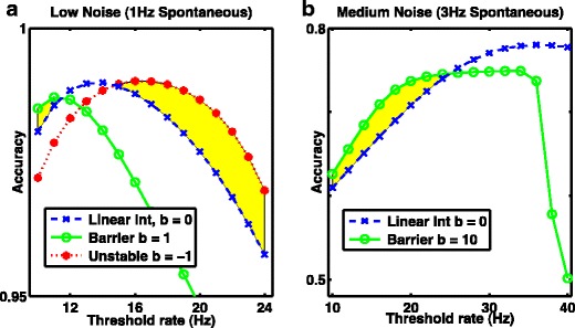
System with greatest accuracy depends on threshold. A system with a positive potential barrier (a stable point attractor) is more accurate when the threshold rate is low, while an inverted potential producing an unstable fixed point is more accurate when the threshold is high. The perfect integrator (linear, no potential barrier) is optimal at intermediate thresholds. a With low noise, D = 100Hz ² s ⁻¹, a low threshold (<20Hz) is optimal, while b with moderate noise, D = 900Hz ² s ⁻¹ a higher threshold (>20Hz) is optimal. a, b Blue dashed curve with crosses: linear integrator, b = 0. Green solid curve with open circles: nonlinear attractor model with barrier, a) b = 1, b) b = 10. a Dotted red curve with asterisks: unstable nonlinear model, b = −1. a, b Regions where nonlinear models are more accurate than the linear integrator are shaded yellow. Results are from 1D system with sextic potential and fixed thresholds with no other readout mechanism, so “undecided trials” are present

Stochastic fluctuations, or noise, are included in the model through a diffusion coefficient, D, which is proportional to the variance in firing rate of the spontaneous state, and is the rate of increase of variance with time in the perfect linear integrator. D contains two main components: 1) internal noise, D _I, within the recurrent circuit that implements any decision-making model and that arises from the high coefficient of variation of spike trains in vivo and the probabilistic nature of vesicle release in synaptic transmission; and 2) signal noise, D _S, in the inputs to the circuit, arising from these same neural processing properties as well as any signal transduction noise in sensory processing. Assuming independence of these two noise sources, the total noise variance is the sum of contributing terms, D = D _I + D _S, or equivalently, D _I = f _I D and D _S = (1 − f _I)D, where f _I is the fraction of total noise arising from sources internal to the circuit. Thus, when we measure a decision-making circuit’s optimal performance by scaling its inputs with a gain factor, g, the signal noise variance scales as g ², while the internal noise remains unchanged, leading to D = f _I D + g ²(1 − f _I)D = D(g ² + f _I − f _I g ²). This dependence, combined with i _d = g i ⁽⁰⁾ _d produces the curves in Figs. 4 and 6 as a function of input gain, g, with different fractions of internal noise, f _I.

Fig. 4.

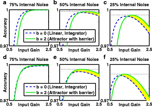
Fixed gain modulation, by scaling up or down the inputs, boosts accuracy. If the decision-making threshold is fixed, then response accuracy can be improved by scaling the input signal and input noise through gain modulation. a–c With moderate total noise (D = 900Hz ² s ⁻¹, equivalent to 3Hz spontaneous activity) in the control system at a gain of unity, accuracy can be increased by reducing the gain (decreasing signal and noise) which slows response times. Highest accuracy is achieved with a point attractor system (green curve) when 50 % or 25 % of the total noise arises from the internal decision-making circuitry. Optimal gain is below unity (to reduce signal and noise) unless more than 50 % of the noise is internal. d–f With low total noise (D = 100Hz ² s ⁻¹, equivalent to 1Hz spontaneous activity) in the control system at a gain of unity, accuracy can be increased by increasing the gain, which speeds up responses. Highest accuracy is achieved with a stable attractor system (green, solid curve) if 50 % of the total noise arises from the internal decision-making circuitry in d), but not 25 % in e-f). a, d 50 % of noise is internal, 50 % from stimulus. b-c, e-f 25 % of noise is internal, 75 % from stimulus. a-b, d-e “Undecided” trials are treated as guesses, ½ correct. c, f) Outcome of “undecided” trials determined by final sign of the decision variable (maximum accuracy). a–f Green solid curve: accuracy for the nonlinear point-attractor model with a barrier, a–c) b = 5, d–f) b = 1. a–f) Blue dashed curve: accuracy for the perfect integrator from the linear model with no barrier, b = 0. Shaded yellow: parameter region where the particular barrier model is more accurate. Black dashed horizontal line: optimal accuracy of attractor-based model

Fig. 6.

The nonlinear attractor-based model with a ramping (urgency) signal produces optimal accuracy even in low-noise systems. a-c Ramping signal, G _u(t) = 2 s ⁻¹, acts to destabilize the symmetric, spontaneous state. d–f Ramping signal causes a dynamic threshold reduction (from 20Hz at t = 0, linearly to zero by stimulus offset at t = 2 s) with G _u(t) = 0. a, d 75 % of the noise is internal, 25 % of noise scales with the stimulus as a function of gain. b, e 50 % of noise is internal, 50 % is input-dependent. c, f 25 % of noise is internal, 75 % is input-dependent. Linear integrator, b = 0. The threshold reduction used in d–f) eliminates undecided trials and “guessing” but the results are qualitatively identical to the use of the urgency signal. a–f Both methods for reducing the numbers of undecided trials boost performance more for the barrier model than the linear integrator (compare b–c and e–f with Fig. 4d–f). Green solid curve: accuracy for the nonlinear point-attractor model with a barrier, t = 2. Blue dashed curve: accuracy for the perfect integrator from the linear model with no barrier, t = 0. Shaded yellow: parameter region where the particular barrier model is more accurate. Black dashed horizontal line: optimal accuracy of attractor-based model

We define the threshold for decision-making—an absorbing boundary at which point the trial ends, with no further processing of inputs—to be at a rate-difference slightly larger than the unstable fixed points of the system. Any input bias produces a linear term in the potential (“tilting” it, Fig. 1). If sufficiently large (compared to the nonlinearity in the system), the bias alone can destabilize the initial (spontaneous) state and that of the non-preferred decision state. In the absence of stochastic noise, such a system’s response would perfectly follow the difference in inputs. By systematically varying the barrier height through the parameter, b we investigate the dynamics of jumps between stable states in comparison to gradual integration when noise is present.

Finally, we note that scaling relationships exist between variables, such that results for given values of noise variance, D, threshold, θ, and stimulus bias, I _D, are identical in the perfect integrator to those with respective values D′ = k ² D, θ′ = kθ and I ^′_D = kI _D To produce identical results in the attractor model, a scaling of the potential (see below) is also required such that U′(r _D) = k ² U(r _D /k) where U(r _D) is the potential describing the original attractor. This first scaling relationship allows a comparison of results with either different thresholds or different stimulus biases. A similar scaling relationship allows a comparison of results with different input durations, as results with noise variance, D, stimulus bias, I _D, and stimulus duration, t _off, are identical for the perfect integrator to those with D′ = k′D, I ^′_D = k ′ I _D and t ^′_off = t _off /k ′. The attractor model’s results are then identical if the effective potential is also scaled, from its original U(r _D) to U′(r _D) = k′U(r _D).

Thus our results with a single value of stimulus strength and duration are generalizable to other conditions.

Trajectories

In order to plot trajectories for the one-dimensional system, we simulate individual instances of the stochastic equation for the variation of rate differences as a function of time (using the forward Euler-Maruyama Method). In this case the dynamics follow:

$$\frac{d{r}_D}{\mathit{dt}}=-\frac{\mathit{dU}\left(r_D,t\right)}{d{r}_D}+\left[G_U\left(t\right)+F\left(t\right)\right]r_D+\sqrt{D}\eta \left(t\right)$$ 1

where η(t) is a white-noise term with zero mean and unit standard deviation, . G _U(t) and F(t) are respectively the urgency-gating signal and the forcing term (see below), each used in a subset of simulations.

Mechanisms of urgency-gating signals

We included an urgency-gating signal in a subset of simulations, on the basis of evidence suggesting stimulus-nonspecific ramping activity during behavioral tasks. Such a signal could provide a ramping additive current to both cell-groups, or could provide a ramping multiplicative gain modulation to all inputs. In the single-variable model, we assess and compare three different implementations of an additive ramping current, as well as one implementation of multiplicative gain modulation, totaling four different versions of urgency-gating signal.

First, we added a destabilizing quadratic term in the potential, G _U(t) in Eq. (1), which increased linearly from zero upon stimulus onset, to mimic an additive current. The motivation for including such an effect of an additive current is found in Eqs. (20–22), which show that in a nonlinear system and additive current destabilizes the spontaneous symmetric state with r _D = 0. We also incorporate such a term in the perfect integrator model of decision-making, as a fair comparison, but doing so renders the model no longer a perfect integrator.

Second, we implemented urgency-gating using the same term, G _U(t) in Eq. (1) to mimic an additive current, but with the trial-averaged linear ramp of gating signal produced by step functions on individual trials. Thus, the time at which G _U(t) stepped from zero to its maximum, was drawn from a uniform probability distribution within the interval of the stimulus duration. Such simulations (data not shown) produced similar, but slightly more accurate responses than those with the linearly ramping input.

Our third method of implementing an additive urgency-gating signal is to decrease the threshold from its standard value at stimulus onset to zero by the end of the stimulus. This third method is instantiated if decisions are reached when the rate of an individual pool in the 2D model reaches a fixed value (rather than the rate-difference between the two pools reaching a fixed value). In such a case, the increase in individual firing rates caused by an additive increase in current leads to a reduction in the threshold for the difference in firing rate (intuitively, the symmetric point with r _D = 0 is closer to threshold if the two cell-groups are firing more, so each closer to their individual thresholds). With such an implementation, the perfect integrator remains a perfect integrator, albeit with dynamic thresholds.

The first and third methods are implementations of two separate consequences of linearly ramping additive current to the full two-variable system. Thus, when we implement an additive urgency-gating signal in the two-variable system, we do not use these separate methods, but simply add the term G _u(t) directly to the separate inputs for each neural group.

Finally, we included a subset of simulations with an urgency-gating signal consisting of a multiplicative increase in the inputs. Assuming a conductance-amplification, we multiplied the signal by [1 + G _u(t)] and the noise variance term, D, by [1 + G _u(t)]² where G _u(t) was a linearly ramping function. Note that, when making a decision based on the difference in two inputs, a multiplicative gain increases the effective stimulus (as the difference in inputs scales with the gain) whereas an additive urgency-gating signal has no impact on the effective stimulus (the difference in inputs is unchanged).

Forcing a choice

In simulations with weak input bias and low noise, the perfect integrator with a fixed threshold may fail to perform optimally simply because it fails to reach the threshold, even though the weight of integrated evidence is biased toward correct choice. However, the attractor model always produces more such “undecided” trials, because it is a “leaky integrator” whose neural firing rates inevitably drift back towards zero (and zero rate difference) in the absence of noise. Thus, compared to chance guessing, any method for producing readout of trials that do not reach threshold has more potential to enhance accuracy of an attractor-based model than the perfect integrator. Models with an urgency-gating signal are less prone to such “undecided” trials, though they still can arise, except if the urgency signal is incorporated by threshold reduction, in which case all trials reach the threshold.

One commonly used manner of “forcing” an “undecided” trial is simply to take the sign of the value of the rate-difference as the indicator of choice (sometimes this is termed the “Interrogation Paradigm” (Bogacz et al. 2006)). While such perfect readout is biologically unlikely, we present the results of such perfect readout in a subset of figures.

We also implemented a forced choice in a more biophysical manner, similar to that with which we implement the additive urgency-gating signal, but with one difference: rather than adding a linearly ramping modest unbiased input to the system (G _U(t) in Eqs. (1–2)), to force a choice, we instead added a large, constant unbiased input for the 100 ms prior to the necessary response time (F(t) in Eqs. (1–2)). That is,

$$U\left(r_D,t\right)=b\left(r_D^2-\beta r_D^4+\gamma r_D^6\right)-I_D\left(t\right)\left(r_D+\mathit{\delta \alpha }{r}_D^3\right)-\epsilon I_S\left(t\right)b{r}_D^2-\left[G_U\left(t\right)+F\left(t\right)\right]r_D^2$$ 2

where F(t) is a step function equal to I _F for t _off − 0.1 < t < t _off and equal to 0 otherwise.

We should point out that our use of F(t) in Eq. (2) allows us to force a choice by causing the final difference in firing rates to move away from zero for all systems, including the perfect integrator. Our analyses show that such a forcing is only easily achievable in a nonlinear system for which the dynamics of rate-differences depend on the total input current. This effect is visible in Eq. (22), as the negative quadratic term in the effective potential that is proportional to the sum of stimulus currents. Such a term appeared in the dynamic equations for the rate difference (Eqs. (16) and (20–21)) and is proportional to the nonlinearity in the firing rate curve for both quadratic and cubic versions. In a linear system, adding additional input equally to two groups has no impact on their difference of firing rates. It is only in the nonlinear attractor formalism above, an equal increase in applied current to all cells in a decision-making network leads to an increase in the difference in firing rates, ultimately forcing a choice. Machens and Brody (Machens et al. 2005) used essentially the same mechanism in a task with three epochs to produce a forced choice following integration of evidence. Even though the rate equations do not justify our inclusion of such a term for the perfect integrator, we do include the term in a model-independent manner so as to avoid any favoring of attractor models.

Compelled response inputs

Most models of tasks with a constant stimulus can reproduce the key results of improved accuracy with increased signal strength of decision-making time, and a unimodal, positively skewed distribution of response times. However, models’ predictions of the effects of temporal variation of the stimulus during decision-making can be more varied. For example, while perfect integrators weight all evidence equally, attractor models give most weight to evidence immediately before the decision; unstable models, meanwhile, give most weight to early information. Thus, examinations of two tasks with non-constant stimuli allowed us to more thoroughly evaluate and compare linear and nonlinear models.

In the first task, stimulus reversal, the sign of the stimulus in the single-variable model is switched at the midpoint of the total duration. Such a switch corresponds to a reversal of direction in a moving-random-dot perceptual experiment (Rüter et al. 2012).

The second task follows a pair of recent studies (Salinas et al. 2010; Shankar et al. 2011), which examined decision-making in monkeys trained to initiate a response (in a two-alternative forced choice task) in advance of the presentation of any information that might indicate which response is correct. In order to simulate such a task, we use the two-variable model with the mean current and any urgency-gating signal, G _U(t) applied equally to the two cell-groups commencing at the start of the simulation but only apply the difference in current at the midpoint, t _off/2, using a total duration of t _off = 500 ms.

Solving the time evolution of the probability density function

In order to assess the decision-making accuracy of different systems over ranges of parameters, our principle method is to solve the time-evolution of the probability density function, P(r _D, t) over a fixed stimulus duration of 2 s in a system with absorbing boundaries marking the decision threshold. The probability density function indicates the likelihood of the rate-difference, r _D, at a particular value at a given time, t. A single calculation of the probability density function can take the place of a large number of simulated trials (and in fact describes the exact probability of any possible outcome for a trial) so its calculation is a much more efficient method for describing the system than brute force simulation.

The dynamics of the probability density function follow the Fokker-Plank equation, which includes two terms (Eq. (3)). The first, diffusive term contains the effects of noise and spreads out the probability density function as time progresses, adding variability. The second, deterministic term causes the system to follow any input bias or move toward an attractor state according to the deterministic rate equations (e.g. Eq. (9)). Thus the Fokker-Plank equation can be written as:

$$\begin{array}{l}\frac{\partial P\left(r_D,t\right)}{\partial t}=-\frac{D}{2}\frac{{\partial }^{2}P\left(r_D,t\right)}{\partial r_D^2}-\frac{\partial }{\partial r_D}\left[P\left(r_D,t\right)\frac{\mathit{dU}\left(r_D,t\right)}{d{r}_D}\right]\hfill \\ \begin{array}{lllllllllllll}\hfill & \hfill & \hfill & \hfill & \hfill & \hfill & \hfill & \hfill & \hfill & \hfill & \hfill & \hfill & =-\frac{D}{2}\frac{{\partial }^{2}P\left(r_D,t\right)}{\partial r_D^2}+\frac{\partial }{\partial r_D}\left[P\left(r_D,t\right)\frac{d{r}_D}{\mathit{dt}}\right]\hfill \end{array}\hfill \end{array}$$ 3

where the effective potential, U(r _D,t), is stimulus-dependent and can in general possess three attractor states (Fig. 1). For our standard parameters, with a choice-threshold set at ±20Hz, we fix the location of attractor states at 0 and ±30Hz with the unstable fixed points at ±17Hz. Our results do not qualitatively depend on these values, so long as the threshold for making a response is not much greater than the highest stable steady states of the system (i.e. a rate-difference of ±30Hz with these parameters). Indeed, quadratic and quartic potentials (with a single steady state at r _D = 0) produce almost identical results to the sextic potential (data not shown). We vary the stability of attractors (i.e. the height of barriers between stable states) through a single parameter, b. This parameter is zero for a perfect integrator, greater than zero for a model with a stable initial state, and less than zero for a model with an unstable initial state.

We assume the probability density function to be initiated as a δ-function at zero rate-difference (P(r _D, 0) = δ(r _D)) denoting a hard reset, so that the firing rates of the two groups are equal at the beginning of any trial. For each time step of the calculation, we accumulate the probability distribution crossing either threshold as the probability that a response has been reached in that time interval. We then set the probability distribution to zero outside the threshold (that is we assume absorbing boundaries and a fixed threshold as suggested by electrophysiological data (Kiani et al. 2008)).

The total fraction of responses categorized as “correct” corresponds to the sum over all time steps of the accumulated probability distribution reaching the positive threshold. The total fraction of responses deemed incorrect is a similar sum of the distribution reaching the negative threshold. We assess percent correct/incorrect and response latencies in a range of networks with different parameters, as shown in Table 1. D in this table is the level of noise variance, which determines likelihood of errors and spread of response times, values of which were chosen to lead to spontaneous firing rates in the absence of inputs, in the range of 1Hz to 5Hz, as is typical of cortical excitatory neurons. The input bias, I _D(t), is the strength of the signal to be integrated. The range of the urgency-gating signal, G _U(t), determines how easily the system can switch from a strongly stable to a strongly unstable spontaneous state over the course of stimulus presentation. The time to stimulus-onset, t _on, determines the amount of variability in the system at the time of stimulus onset. In the majority of protocols, the stimulus remained for a fixed duration, up to a time, t _off, at which time we either forced a response (see above) or assigned “undecided” trials (the fraction that had not reached threshold) equally as “correct” or “error” trials, or assigned all trials with a final value of r _D > 0 as correct and those with r _D < 0 as incorrect (perfect mathematical readout).

Table 1.

Parameters for Fokker-Planck equations for 1-D effective potential

Parameter	Symbol	Standard Value	Range	Units
Diffusion constant (noise variance)	D	900	100; 900; 2500	Hz 2 s −1
Bias term	i D	20	20	–
Stimulus duration	t off	2	2–∞	s
Choice threshold	θ	20	10–100	Hz
Time constant	τ	0.010	0.010	s
Quadratic term	α	0–60	0–60	–
Quartic factor	β	4/900	4/900; 1/900	–
Sextic factor	γ	β/1200	β/1200; β/4800	–
Urgency gating maximum	G maxU	0	0–20	–
Forcing term	I F	0	0; 200	–
Input gain	g	1	0–3	–
Internal fraction of noise	f I	N/A	0.25, 0.5, 0.75	–

Probability density function for two variables (2D)

To ensure that our results for the single-variable system with an effective potential apply to the complete system with two variables (Table 2), we went on to simulate the evolution of the probability density function using the two rate variables, r ₁ and r ₂ (rather than just their difference, r _D = r ₁ − r ₂). Equations (6) and (17) describe the deterministic terms ($\frac{d{r}_1}{\mathit{dr}}\mathrm{and}\frac{d{r}_2}{\mathit{dt}}$). Adding a diffusion term (D′ = D/2) leads to:

$$\frac{\partial P\left(r_1,r_2,t\right)}{\partial t}=-\frac{D\prime }{2}\left[\frac{{\partial }^{2}P}{\partial r_1^2}+\frac{{\partial }^{2}P}{\partial r_2^2}\right]+\frac{\partial }{\partial r_1}\left[P\frac{d{r}_1}{\mathit{dt}}\right]+\frac{\partial }{\partial r_2}\left[P\frac{d{r}_2}{\mathit{dt}}\right]$$ 4

Table 2.

Parameters for 2-D Fokker-Planck equations

Parameter	Symbol	Standard Value	Range	Units
Diffusion constant (noise variance)	D′ = D/2	450	50; 450; 1250	Hz 2 s −1
Choice threshold	θ	20	20	Hz
Time constant	τ	0.010	0.010	s
Maximum rate	r M	100	100	Hz
Maximum current	I M	200	200	–
Sum of stimuli	I S	40	40–80	–
Bias of stimuli	I D	0.8	0.8	–
Stimulus Duration	t off	2	0.1–∞	s
Nonlinearity	b	0–0.5	0–0.5	–

We simulated the system on a discrete mesh with Δr = 0.2Hz, and confirmed key results using a finer mesh (Δr = 0.05Hz). Similarly we confirmed all results to be accurate to better than 1 part in 1000 with a decrease in Δt by a factor of 10 and to match the equivalent one-dimensional simulations of a quartic potential (Eq. (22)).

Simulation details

We simulated all dynamical equations in Matlab (Mathworks, Natick, MA) using the forward Euler-Maruyama method. Time steps, Δt, were chosen such that results did not change by more than 1 part in 10,000 using a 10-fold lower time step. This led to Δt = 2 × 10⁻⁶  s for all cases with D = 2500Hz ² s ⁻¹and Δt = 5 × 10⁻⁵  s for D = 100Hz ² s ⁻¹ in the absence of a forcing current and Δt = 1 × 10⁻⁵  s in all other cases. For Fokker-Plank simulations the “spatial” grid used Δr _D = 0.2Hz, though key results were verified (unchanged to 1 part in 1000) using a finer mesh with Δr _D = 0.05Hz. Code is available by visiting the website: http://people.brandeis.edu/~pmiller/Decision_code.

Results

Optimality of single-variable models

Single variable models are those in which the difference in firing rates is the only variable of importance—i. e., in which the dynamics of the system and response times depend only on the rate-difference between two neural groups. For such models an effective potential can be produced whose slope describes the direction of deterministic change in rate-difference. A static model is one whose parameters do not change over time—equivalently, after stimulus onset the effective potential is static. This represents a neural circuit with fixed connections responding to a constant input, and thus does not contain any urgency-gating signal. Below, we examine optimality in this sort of model, describing first the basic result and then the results of various parameter manipulations.

Decision-making accuracy with attractors and barriers to diffusion

In our standard simulations, starting with a “moderate” noise level of D = 900Hz ² s ⁻¹, we find that increasing the nonlinearity factor from zero—i. e., turning the network from an ideal integrator into a network that hops from attractor to attractor—improved accuracy (Fig. 2a, solid green trace). The nonlinearity factor produces a barrier to noise-driven diffusion, reducing the spread of the probability distribution. This had two, opposing results. First, noise-driven errors—namely incorrect responses—became rarer with increasing barrier height (Fig. 2a, dashed red trace). At the same time, the number of “undecided” trials, for which threshold is not reached in the allotted 2 s of decision time, increased with barrier height (Fig. 2a, dot-dashed magenta trace); beyond an optimal barrier height, the mean response time took longer than the allowed decision time. However, for a range of barrier heights, the dominant effect was reduction in the error probability—the greatest accuracy was achieved with a non-zero barrier.

Fig. 2.

Probability of incorrect response decreases with increasing height of effective potential barrier. a Moderate noise, D = 900Hz ² s ⁻¹, equivalent to 3Hz spontaneous activity. b Low noise, D = 100Hz ² s ⁻¹, equivalent to 1Hz spontaneous activity. a, b Dotted blue = correct responses; Dashed red = incorrect responses; Dot-dashed magenta = no response (undecided); Solid green = minimum accuracy = correct + (undecided)/2; Solid black = maximum accuracy = probability of final rate greater than zero. Results are from 1D system with sextic potential and fixed thresholds

In the lower-noise system (D = 100 Hz ² s ⁻¹) introduction of a barrier via a positive nonlinearity did not improve accuracy (Fig. 2b, solid green trace), because even without a barrier to diffusion of firing rates, the threshold was often not reached within the 2 s of integration time. Thus, the number of undecided trials (Fig. 2b, dot-dashed magenta trace), rather than the number of incorrect responses (Fig. 2b, dashed red trace), became the rate-limiting factor on accuracy in this case.

The negative impact of undecided trials in models with a barrier to diffusion is greatly ameliorated if the response can be determined by a perfect readout of the final sign of the decision variable (Fig. 2b, solid black trace). Since such perfect readout is unlikely in a real biological system, in later sections we will assess how biologically plausible mechanisms can improve accuracy of otherwise “undecided” trials towards that of a perfect readout.

To summarize, Fig. 2 shows that given a specific fixed input, a specific fixed threshold and a specific time limit for responses, an integrator can be, but need not, be the most accurate model, even though adding that time limit causes more “undecided” trials in the nonlinear model. Adding a barrier in Fig. 2a improves accuracy because it slows responses; the integrator responds in much less time than the 2 s available, but more of the quickest responses are errors.

Adjustment of response times via changing the location of a fixed threshold

In a later section we will go more deeply into an assessment of optimality when taking response time into account, but in the following two subsections we examine methods whereby the system could be improved simply by optimizing static parameters. We assess two methods that have reasonable claims to biological plausibility, namely adjustment of the decision threshold (as in (Lo and Wang 2006; Simen et al. 2006; Simen et al. 2009; Bogacz et al. 2010)—this subsection) and modulation of input gain (as in (Brown et al. 2005; Shea-Brown et al. 2008; Eckhoff et al. 2009)—see next subsection).

We assessed the system’s accuracy as a function of the static decision-making threshold—i.e. the firing rate needed to produce a response—under both low noise conditions (in which the perfect integrator produced many “undecided” responses) and high noise conditions (in which the perfect integrator reached threshold too quickly compared to the time available for stimulus integration). In the system with low noise, we found that the accuracy of the perfect integrator was greatest at a threshold below the standard level used in Fig. 2 (20Hz), while the optimal accuracy of a system with moderate noise was achieved at a threshold above the standard level. In both low and moderate noise, parametric variation of the threshold demonstrated the optimal accuracy of the perfect integrator was better than the optimal accuracy of any nonlinear system with a static barrier produced by a positive nonlinearity (Fig. 3a, dashed blue versus solid green traces). Rendering the initial state unstable via a negative nonlinearity, however, reliably resulted in improved accuracy and the highest absolute accuracy, for a non-integrator (Fig. 3a, dotted red trace). Yellow regions represent improvement in accuracy realized by inclusion of non-linearity.

Optimal performance via adjusting the level of a fixed input gain is constrained by internal circuit noise

The early stages of sensory processing modulate the amplitude and gain of any external signal, quite possibly moving them toward the optimal range for later processing. Indeed, it has been suggested that one function of norepinephrine is to produce precisely such gain modulation of the inputs to and within the decision-making circuitry (Brown et al. 2005; Eckhoff et al. 2009). Thus it is reasonable to ask what effect scaling of the inputs—and of any associated noise—has on accuracy, and whether optimization of this static parameter favors integrators, stable attractors, or unstable fixed points.

Of course, the “associated noise” is actually a sum of two sources of noise—input and internal (i.e. within the decision-making circuit). The former of these most likely scales with input gain (Gold and Shadlen 2000, 2003), while the latter does not. We therefore examined how performance was affected by parametric adjustments of the proportion of the total noise making up each fraction. Specifically, for a given proportion of internal noise at a gain of unity, whose value we held constant, we scaled both the input signal and the standard deviation of the input noise by a factor—the input gain—that we parametrically varied. Such an effect would arise by a scaling of the conductance of afferent synapses.

We found, in the system which possessed “medium” noise at a gain of unity, that the optimal accuracy of the model with a stable attractor and barrier (Fig. 4, solid green traces) is higher than that of the integrator (Fig. 4, dashed blue traces), except at a very low fraction (≤ 10 %) of internal noise (Fig. 4a–c). This medium noise system benefits from a reduction of input gain, because in our standard protocol (with a gain of unity) decisions were made more quickly—and thus with more errors—than is optimal. Reductions in input gain (which reduce the signal) can improve decision-making accuracy when they reduce the noise in the system sufficiently.

Since “undecided” trials are rare in the system with medium noise, implementing a perfect readout of the final state of the system (Fig. 4c, the maximum accuracy condition) has little impact on these results, except to further enhance the advantage of the attractor model (which has more undecided trials) over the perfect integrator.

Reduction of noise helps the attractor model less, because noise actually drives the stochastic transitions constituting a decision. Thus in Fig. 4b at the lowest input gains, the barrier model is more accurate if more noise is internal, so not scaled away (compare Fig. 4b green trace near zero gain with the same trace in Fig. 4a). Such a seemingly paradoxical result of enhanced accuracy with decreased signal to noise ratio, seen also in our spiking-neuron simulations of the task (Miller and Katz 2010), is actually a reliable phenomenon, akin to stochastic resonance, often observed in models with a stable initial state (Gammaitoni and Hänggi 1998; Gluckman et al. 1998; McDonnell and Abbott 2009; Miller and Katz 2010).

For the low noise system, optimal accuracy for the integrator (Fig. 4d–f, dashed blue traces) is below that of the attractor model with a barrier (Fig. 4d–f, solid green traces) if internal noise is > 50 % of the total, though differences between the two are miniscule. In the standard system (i. e. with unit gain) with low noise, accuracy is limited by the number of undecided trials, and thus improves as gains increase from unity. The improvement is larger if the increase in signal does not come with a concomitant increase in noise, which is the case when the dominant contribution to the noise is internal (compare Fig. 4d and e). If the “undecided” trials are settled based on the sign of the decision variable (i.e. the maximum accuracy condition, Fig. 4f) then accuracy increases considerably in all systems, but more so for the attractor model, such that it’s accuracy matches the perfect integrator even if only 25 % of the noise is internal. Since performance in the attractor system (under standard conditions) was more limited by undecided trials than was performance of the perfect integrator, in all cases the attractor system benefits more by any increase above unit gain (Fig. 4d–f, solid green traces), so the already-observed advantage over the perfect integrator only increases (Fig. 4d).

In summary, if a noise-free circuit were possible, the integrator could produce optimal accuracy, but if even a relatively small fraction (≥ 15 % of D = 900Hz ² s ⁻¹) of the total noise in the decision-making circuitry is internal rather than arising from inputs, non-integrators achieve greater accuracy than the perfect integrator.

Decision-making accuracy in models with an urgency-gating signal

An urgency-gating signal is a method for speeding up the likelihood of a response as time passes, and for settling otherwise undecided trials. It has been suggested to explain behavioral data in some tasks (Cisek et al. 2009), and has been further suggested to allow greater accuracy in decision-making tasks than a true perfect integrator (Standage et al. 2011). The urgency-gating signal can be instantiated as a ramping multiplicative gain in the inputs, or a lowering of threshold with time, or a reduction of the stability of the initial, undecided state with time. We investigate and provide results for all three alternatives (and justify the third one, since it is novel).

In nonlinear models with an initial point attractor and barrier the initial, undecided state will be destabilized by a ramping input current (Eqs. (21–22)), increasing the likelihood of response. Moreover, such a ramping input current can multiplicatively increase the effect of any input bias (Eqs. (21–22)), thus providing a particularly simple biological implementation of urgency-gating. Such an unbiased ramping input current has no effect on rate-differences in a linear, perfect integrator, but to ensure a fair comparison, we added equivalent urgency signals to every single-variable model (see Methods). To summarize, we implement the urgency signal, equally for all types of barrier, either as a linearly increasing term, which destabilizes the initial spontaneous state (Fig. 5, dot-dashed green curve), or as a linearly decreasing threshold, which reaches zero by the end of the stimulus (Fig. 5, dashed red traces).

Fig. 5.

Addition of a ramping (urgency) signal boosts optimal accuracy and favors increased barrier height. a For the low noise system (D = 100Hz ² s ⁻¹) the urgency gating signal boosts performance for both linear integrator (b = 0) and point attractor models (b > 0), though more so for larger barriers, such that optimal accuracy arises in a model with a barrier (black asterix, b = 1). An urgency signal that destabilizes the initial state (dot-dashed, green trace, G _u(t) = 1.5 t) can produce greater accuracy than one that causes a reduction in thresholds (dashed red trace). b For the moderate noise system D = 900Hz ² s ⁻¹, a destabilizing urgency gating signal (dot-dashed green trace, G _u(t) = 5 t) reduces accuracy for the linear integrator (b = 0) but boosts accuracy for models with a large barrier, increasing optimal accuracy and increasing the optimal barrier height (black asterix, b = 18). An urgency signal which acts to reduce thresholds (dashed red trace) is less accurate, but again its optimal accuracy is for an attractor model with a barrier. Both forms of urgency signal cause threshold to be reached in over 99.9 % of trials for linear integrators and for nonlinear barrier systems, so “undecided trials” are lost. a–b Blue solid curve: no urgency signal. Red dashed curve: urgency signal by linearly ramping reduction of thresholds to zero. Green dot-dashed curve: urgency signal by slowly increasing the destabilization of the initial state

We find that optimal accuracy (Fig. 5 black asterisks on dot-dashed green traces) is achieved when nonlinearity provides a diffusive barrier such that the urgency-gating signal does not render the initial attractor state unstable until near the end of the stimulus duration. In all simulation conditions, an appropriate combination of barrier height and urgency-gating signal could be found that produced better accuracy than a perfect integrator (Fig. 5, y-intercepts), even one with linearly decreasing thresholds (Fig. 5, dashed red). Similarly, when we parametrically varied the level of the static threshold (as in Fig. 3), we ubiquitously found that some model with a positive nonlinearity to produce an initial barrier, combined with an urgency-gating signal, always produced greatest accuracy (data not shown).

In fact, a nonlinear, temporally varying system could perform better than the perfect integrator even when thresholds were specifically chosen to be optimal for the integrator and unchanged thereafter. In a system with high noise (D = 2500Hz ² s ⁻¹, corresponding to 5Hz spontaneous activity), for instance, the optimal threshold for the perfect integrator was found at a rate higher than that of the high-rate attractor states of the sextic potential. Such a rate prevented decisions from being made (and producing chance performance) given moderate nonlinearity. However, an alternative potential with attractor states at r _D = ±80Hz enabled a nonlinear system to reach the high threshold of 60Hz and perform better than the perfect integrator.

Our main result—optimal accuracy arises from a combination of an attractor model with an urgency-gating signal—was maintained when we parametrically varied the fixed input gain (Fig. 6, solid green curves). In Fig. 6 we present the results for the low-noise system (the only case where the perfect integrator was more accurate than the attractor model in our standard conditions), and find than with the inclusion of an urgency-gating signal an attractor model (solid green curve) produces optimal accuracy, regardless of whether the signal is implemented by destabilizing the initial state (Fig. 6a–c) or by linearly decreasing thresholds to zero (Fig. 6d–f), and regardless of whether the system is dominated by internal noise (Fig. 6a,d) or by input noise (Fig. 6c,f).

Decision-making accuracy when responses are forced

The long-standing analytic proof (Wald 1947; Wald and Wolfowitz 1948) of perfect integration as the optimal process for making a two-alternative forced choice for any fixed time interval (and conversely the process requiring the minimum time to reach a given accuracy) assumes either an unlimited duration with fixed thresholds, or an absence of threshold combined with a readout that perfectly responds to any difference in total accumulation of inputs.

A biological readout mechanism, however, is unlikely to reproduce such perfect analytic results. More likely is something resembling the mechanisms that we instantiate above, or the one below, wherein we force a response in such trials by rendering the undecided state of low firing rate difference unstable—by “forcing” a response to threshold. Such instability would arise in practice via a strong global input current in any nonlinear model.

A forcing term applied in the final 100 ms of the trial (instantiated as a large, negative quadratic addition to the effective potential, see Methods) led to qualitatively the same result as an urgency-gating signal, in that it improved accuracy of nonlinear models more than perfect integrators. The fraction of undecided trials fell to below 10⁻⁸ in all cases—a change favoring attractor models, which otherwise generated more undecided trials. Even in the low noise case, if 50 % of the noise is internal then at an optimal level of gain, an attractor model with a barrier (b = 1) is more accurate than the perfect integrator.

It might appear surprising that such a forcing term would produce better than chance responses from undecided trials in a barrier model—after all, while the system remains in its initial stable state, it has not integrated any of the prior input. However, the boost in accuracy provided by the forcing term can be understood from the shape of the effective potential prior to addition of the forcing term (Fig. 7a1–c1). The biasing current causes the stable “undecided” state to be offset from zero on the side of correct responses. Thus, when a response is forced, the otherwise undecided responses will more likely become correct responses than errors. This shift in the stable fixed point—which marks the peaks of the probability distribution for “undecided” trials—also explains why perfect readout improves performance for the barrier model beyond chance guessing, in Figs. 2 and 4c, f. Since the barrier model typically has more undecided responses without a forcing term, then the benefit of a forcing term can favor the barrier model more than a perfect integrator.

Fig. 7.

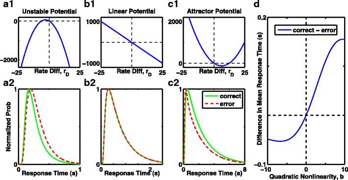
Expectation of faster or slower error responses depends on curvature of the nonlinear 1D model. a1), b1), c1) Effective potentials include a bias current, which produces correct responses at positive rate-difference r _D. a1) Fixed point of the unstable potential (where dr _D/dt = 0) is shifted left of the origin, so crossed on error but not correct trials, leading to slower error responses in a2. b1) Linear potential has constant gradient, leading to equal shapes of correct and error response distributions in b2. c1) Stable fixed point of the potential with a barrier is shifted to the right, so crossed on correct, but not error trials, leading to slower correct responses compared to errors in c2. a2), b2, c2) The corresponding response time distributions (scaled to a peak of 1, for easy comparison of the shapes—the number of errors is so much fewer than number of correct responses that shapes of the original distributions can not be visibly compared). Green solid curves: scaled distribution of correct response times. Red dashed curves: scaled distribution of error response times. a1), a2) b = −1. b1), b2) b = 0. c1), c2) b = 1. D Summary of the difference in mean response times as a function of quadratic curvature of the effective potential, or the stability of the initial fixed point (negative curvature is unstable, positive curvature is stable, zero curvature is marginally stable and equivalent to an integrator). Systems with an unstable fixed point produce slower errors, while systems with a stable fixed point produce faster errors. Simulations contained no fixed time limit, so a threshold was always reached

Explaining the above: the role of response time distributions for non-integrators and integrators

Given that the perfect integrator is often described to provide the optimal trade-off between mean reaction time and accuracy, it is quite reasonable to ask why we observe higher accuracy with a nonlinear system combined with an urgency-gating signal in all circumstances. The answer to this question can be found in examinations of simulations with a range of input currents and no time limit for decision-making. For both the perfect integrator and the nonlinear system, accuracy increased and reaction time decreased with increased input bias (input bias being the difference in input currents, representing coherence in motion tasks). At high input bias the nonlinear model with urgency-gating is more accurate than the linear integrator, although reaction time is slower; this situation reverses at low input bias, when the slower input-induced dynamics allow more time for the urgency-gating signal to effect a response. Figure 8a summarizes these data, showing that there is no input bias for which the nonlinear system produces both higher accuracy (Fig. 8a, dashed blue trace) and faster mean response times (Fig. 8a, green trace) than the perfect integrator. On the contrary, as expected, for all combinations of nonlinear system assessed, we found a small range of inputs for which the perfect integrator did produce more correct responses with a faster reaction time—just as predicted by standard theory.

Fig. 8.

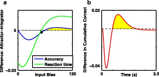
Mean response time or accuracy, but not both, can be improved with a nonlinear system and urgency-gating signal. a Difference in accuracy (blue) and difference in mean response time in units of seconds (green) between the nonlinear system with urgency-gating signal (NL + Urgency, which has discrete attractor states after stimulus onset at low input bias), and the perfect integrator as a function of input bias. b Difference in cumulative distribution of correct responses over the course of the stimulus presentation with a fixed input bias of 58 (black asterix in a), where mean response times are approximately equal, but performance is slightly higher with the perfect integrator. Note the middle epoch (shaded yellow) denoting the range of times for which the nonlinear system has produced more correct responses. Thus the nonlinear system with urgency-gating signal can produce better performance for fixed stimulus durations within this time interval. a–b All curves are with moderate noise, D = 900Hz ² s ⁻¹ and response threshold, θ = 20. The perfect integrator is linear with b = 0 and G _U(t) = 0 while the system with discrete attractors is nonlinear with a barrier given by b = 5 and has an added urgency-gating signal of G _U(t) = 7.5 t. In order to obtain the full response time distribution, stimulus duration was not limited, so threshold was always reached

Any apparent contradiction with our prior results is resolved in Fig. 8b, which shows the cumulative fraction of correct responses for two systems with the same mean response times. Since the shapes of the distribution of response times differ between nonlinear and integrator systems, there is a range of response times for which the nonlinear system with urgency gating produces more correct responses than the perfect integrator, even if eventually, once all responses are produced and counted, the perfect integrator is more accurate. This effect arises because the response time distribution of the perfect integrator has greater skew—for the same mean response time the integrator has more very slow responses—a simple and direct consequence of the urgency signal ensuring responses are timely. Thus, it is the limited stimulus duration with fixed response time that allowed us to recognize nonlinear systems with an urgency signal to have consistently greater accuracy than the perfect integrator (Fig. 8b).

Rate of accumulation of reward in the absence of a time limit

By limiting stimulus duration and response time, one necessarily affects the number of rewards that can be delivered (and achieved) within a particular length session. This variable is commonly known as the “reward rate.” Optimization of performance in decision-making tasks is the same as maximization of reward rate. Manipulation of the maximum achievable reward rate also has an impact on the optimal model, which we explore below.

In decision-making tasks with no fixed response time, the maximum achievable reward rate can be manipulated by varying the inter-trial interval (ITI), because the reward rate is equal to the probability of being correct (the accuracy) divided by the total time per trial (mean response time plus ITI) (Swensson 1972; Balci et al. 2011). The ITI determines where one should operate in the speed-accuracy tradeoff. When the ITI is long compared to the decision-making time, it is more important to take the time to be accurate, as each error is relatively costly; if the ITI is short, meanwhile, it can be worth making more errors, as the increase in the rate of trials initiated in a given period may compensate for the errors. Thus, when measuring reward rate in the absence of any constraints on stimulus duration or response time, an unstable, fast but error-prone system is optimal when the ITI is short (Fig. 9a, solid red trace), whereas the more accurate but slower attractor system is optimal when the ITI is long (Fig. 9a, dashed blue trace). The perfect integrator, meanwhile, is optimal at just a single, specific value of intermediate ITI (in this case approximately 5 s—Fig. 9a, dot-dashed green trace).

Fig. 9.

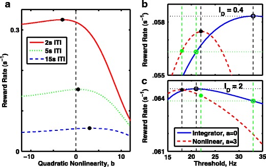
Optimal performance, measured as mean reward rate, depends on the inter-trial interval, the stimulus bias and threshold rate. a In the absence of a time limit for decisions, so threshold is always reached, reward rate is maximized with an unstable system (negative quadratic curvature), which forces faster, less-accurate responses is the inter-trial interval (ITI) is low (e.g. 2 s, red curve) but is maximized with a stable point attractor (positive curvature, indicating a barrier) if slower responses are less penalized due to a long inter-trial interval (e.g. 15 s, blue curve). A perfect integrator, exemplified by the linear system (curvature = 0, vertical dashed line) is optimal at a single, specific inter-trial interval, slightly less than 5 s (green line). All curves are with D = 400Hz ² s ⁻¹, with stimulus bias, i _D = 20 and with threshold, θ = 20Hz. Red solid curve: ITI = 2 s. Green dot-dashed curve: ITI = 5 s. Blue dashed curve: ITI = 15 s. The absence of time limit ensures an absence of “undecided” trials. b, c Reward rate with an ITI of 15 s for the perfect integrator (blue solid curve) and a barrier model (red dashed curve) as a function of static threshold. b Standard stimulus bias, i _D = 20. c Large stimulus bias, i _D = 50, leads to lower value for the optimal threshold rate. b, c Blue solid curve, linear integrator with a = 0; red dashed curve, nonlinear model with a = 3; black open circle, performance of linear integrator when threshold is optimal; black asterisk, performance of nonlinear model when threshold is optimal; green open circle, performance of linear integrator when threshold is optimal for the alternative stimulus; green asterisk, performance of nonlinear model when threshold is optimal for the other stimulus

For all systems studied in this situation with no fixed time limit, an optimal reward rate was achieved without an urgency signal. The primary consequence of an urgency-gating signal was to increase the barrier height corresponding to the maximum reward rate (i.e. shifted the peaks of curves in Fig. 9a to the right). However, the overall maximum reward rate was slightly reduced in these cases (data not shown). This result can be understood if the urgency-gating signal is characterized as a way to ensure a response in a given time window, so the signal is of value when stimulus duration or the time window for response is fixed.

The results of Fig. 9a were all produced with a fixed static threshold. Given our results in Figs. 3 and 8, as well as longstanding theoretical proofs (Wald 1947; Wald and Wolfowitz 1948), one might expect that for any particular fixed level of input an optimal threshold can be chosen for the integrator so that its rate of reward accumulation is greater than that of any other system. Indeed, this is the case: we show two examples in Fig. 9b–c, in which, with a 15 s ITI, the perfect linear integrator can be made to outperform the barrier model. Figure 9b demonstrates results for the same signal used in Fig. 9a, where the barrier model accumulates reward more rapidly at a threshold of 20Hz, because the integrators optimal threshold is much higher, at 35Hz. However, it is worth pointing out that with stronger input bias (just as with reduced ITI) the optimal threshold is lower for all systems. In fact the optimal threshold shifts more with changes in input for the linear perfect integrator than it does for the barrier model (compare Fig. 9b with Fig. 9c). Thus we find that even though the perfect integrator performs better when both systems are optimized for a given input and ITI, under many changes in the task—such as with a new input strength—one can easily find that the barrier model performs better than the perfect integrator at the previously optimized thresholds (green asterisks are higher than green circles in both Fig. 9b and c). Thus, in a laboratory setting with over-trained animals, where the inputs and task design have been learned over weeks or months, the integrator model will likely be optimal; in a natural environment however, in which the typical strength and frequency of an input may not be known a priori, the barrier model will likely be optimal.

Extending our results to two-variable models

All of the above results made use of a model with a one-dimensional (1D) effective potential. To extend and validate these results, we also simulated the full two-variable system, using a firing-rate curve that could range from linear (α = 0) to cubic (α = 1) (Fig. 10a). In so doing, we were able to map from a perfect integrator to an attractor-based system with a fixed point at the origin. At the broadest level, the results of these latter simulations are simple to describe: the two-variable system recapitulates the results of the 1D system (i. e., demonstrating the frequent sub-optimality of the perfect integrator).

Fig. 10.

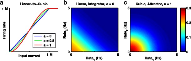
Models for a 2-variable decision-making from linear, perfect integrator to cubic, nonlinear attractor. a The parameter a, dictates the degree of nonlinearity, by adding a cubic term to the piece-wise linear portion of the firing-rate curve. b, c The steady state probability distribution of the pair of firing rates in the absence of input for the linear perfect integrator in b and the cubic nonlinear model in c. Spontaneous rates are constrained in the 2D system (unlike the perfect integrator in 1D) because of the threshold nonlinearity at zero rate (firing rates can not be negative, so noise-driven drift is constrained). b For the linear system (perfect integrator) for a given sum of the two rates, the probability density is independent of the difference in firing rates, whereas c) the nonlinear system constrains the difference in firing rates to produce elliptical contours of constant probability. Results are with D′ = 450Hz ² s ⁻¹, equivalent to D = 900Hz ² s ⁻¹ in the 1D system. Steady state distributions are shown, so no time-limit is included

Advantages of the two-variable model

The full two-variable model, while more computationally intensive, provided at least 3 advantages over the single variable model: First, use of the 2-variable system allowed us to directly relate the level of noise in the system to the range of spontaneous firing rates prior to stimulus presentation, demonstrating that the low noise and medium noise simulations used here correspond to approximate levels of 1Hz or 3Hz spontaneous activity respectively (see Appendix D); second, it allowed us to test the dependence of our main conclusions on whether fixed thresholds were separate for each group (i.e. if either r ₁ or r ₂ reach a threshold, a situation akin to competing accumulator models of decision-making or race models) or based on the difference in firing rates (i.e. if r _D = r ₁ − r ₂ reaches a threshold, as occurs in the 1D system and the drift diffusion model); third, and arguably of greatest importance, it allowed us to relax constraints needed in the 1-dimensional system to ensure that the difference in firing rates did not depend on the sum of rates (see Requirements for an Effective Potential in Appendix B)—in particular the requirement ε = (W _S − W _x) = 0 that led to Eqs. (2) and (20), an essential condition for a single-variable nonlinear model—and thus to study the robustness of linear and nonlinear systems to mistuning of parameters (Fig. 11).

Fig. 11.

Robustness to mistuning increases with nonlinearity and an urgency-gating signal in 2D system. a Linear system (a = 0, blue dashed curve) is a perfect integrator with balanced cross-inhibition (W _X = 0.5 where it outperforms the nonlinear system (green solid curve). With increased cross-inhibition (reducing stability) the nonlinear system (which enhances stability of the spontaneous state) is more accurate than the linear system. Note that in both cases, accuracy of the most optimal system (peaks of curves) exceeds that of the perfect integrator (linear, W _X = 0.5). b Urgency-gating is included as a multiplicative gain term (max = 1, leading to an eventual doubling of stimulus and 4-fold increase in). The ramping multiplicative gain improves performance of the linear system but the nonlinear system with an initial barrier has the higher optimal accuracy. c Urgency-gating (max = 0.1) is included by an additional unbiased ramping current, with decision-threshold set at a fixed rate-difference (|r ₁ − r ₂| = 20Hz). Performance of the linear system deteriorates rapidly with imperfect tuning, and it is unaffected by an urgency-gating signal. The nonlinear system with attractors is more robust to a decrease in cross-inhibition, where its performance is significantly boosted by the urgency-gating signal (compare with a). d Urgency-gating included exactly as in c) but thresholds are at fixed individual population rates (r ₁ = 20Hz or r ₂ = 20Hz). a–d Dashed blue curve with asterisks: linear system with . Solid green curve with open circles: nonlinear attractor-based system with a = 0.1. Yellow shaded area indicates the range of parameters where the nonlinear system outperforms the linear system (which produces a perfect integrator at W _X = 0.5). Low-noise, D′ = 50Hz ² s ⁻¹ (equivalent to D = 100Hz ² s ⁻¹ in the 1D system and 1Hz spontaneous activity) with a fixed duration of 2 s. Panels a-c) include the effect of “undecided” trials, while the urgency signals in panel d) ensure threshold is reached on over 99.9 % of trials

Robustness to parameter mistuning

Perfect integration requires perfect tuning of parameters (δ = 0 in Eq. (9)). Since such perfect tuning is unlikely in a real biological system (a fact that is widely discussed in the literature (Renart et al. 2003; Meyer-Baese et al. 2009; Bouvrie and Slotine 2011)), it is important to assess how accuracy of our various models—the linear system, a static nonlinear system, and a nonlinear system combined with an urgency-gating signal—deteriorate with mistuning. The answer, as shown in Fig. 11, is clear: across a variation of ±10 % in the level of cross-inhibition, the nonlinear system with an urgency-gating signal (Fig. 11, solid green traces)—instantiated as either a ramping input current (Fig. 11c–d) or a ramping input gain (Fig. 11b)—was most robust than a linear integrator, and produced the highest level of accuracy across the parameter range.

Thresholds of single-group firing rate versus firing rate difference

The two-variable system allows us to assess whether a model with separate fixed thresholds for each group (i.e. if either r ₁ or r ₂ reach a threshold, a situation akin to competing accumulator models of decision-making or race models) performs differently from a system with a threshold based on the difference in firing rates (i.e. if r _D = r ₁ − r ₂ reaches a threshold, as occurs in the 1D system and the drift diffusion model). It might be reasonable to expect such differences, because an input current could conceivably raise the rates of two cell-groups nearly equally, failing to appreciably increase the difference in their firing rates, but causing a response based on reaching a single group’s individual firing rate threshold.

In reality, however, basing the decision-making threshold on the individual firing rate of a group of neurons, rather than the firing-rate difference between groups, introduced few qualitative differences in accuracy of nonlinear systems, although in the presence of either an urgency-gating (ramping) input or an input forcing a response the type of threshold did matter for the accuracy of a linear system. Since adding an additional, symmetric input current has no effect on the difference in firing rates of a linear system (unlike the nonlinear system), such an urgency-gating or forcing current is ineffective in the linear system if the threshold is based on difference in firing rate. However, when the threshold is an absolute firing rate, the additional input current does indeed hasten a decision in the linear system, boosting accuracy. Such a situation corresponds to a monotonic decrease in threshold with time for the 1D linear model—a manipulation that favored the attractor model over the perfect integrator. Indeed, we found that accuracy in a 2D linear system with an urgency-gating current and individual rate thresholds (Fig. 11d) resembles that of a linear system with urgency gating via input gain and rate-difference thresholds (shown in Fig. 11b, dashed blue trace) and was similarly bested by the nonlinear attractor model (Fig. 11d, solid green trace).

Forcing a response in the 2-variable system

Given the finite time window for making a response, we found on many trials that threshold was not reached within the response window. We treated such trials as driving a random response. However, the perfect integrator always maximized the probability that r ₁ > r ₂ for a fixed duration of stimulus with I ₁ > I ₂, so by treating trials with r ₁ > r ₂ as chance when threshold was not reached, it could be argued that we may have unfairly disadvantaged this model. To examine this possibility, we added an input to the system to force a response based on the final rates, expecting that such a forced response could favor the integrator in all situations.

To achieve this, we added a “forcing current” in the last 100 ms of a 2-s stimulus period. We simulated the best-case scenario for the perfect integrator using the low-noise case, for which it produced more undecided responses than the optimal nonlinear urgency-gating model (and thus could benefit most from the “forcing” of undecided responses).

In the case where the threshold was one of rate-difference, a forcing-current, like an urgency-gating signal has no effect in the linear system (the perfect integrator), since the rate-difference is independent of the sum of input currents. On the other hand, in the nonlinear system, such a forcing-term improved optimal accuracy (data not shown) by reducing the number of undecided trials.

To further favor the perfect integrator, we used fixed population-rate thresholds—i.e. a decision is made depending whether r ₁ or r ₂ first reaches threshold, irrespective of magnitude of the difference, r ₁ − r ₂. We found that adding a forcing current with such thresholds improved accuracy considerably, to 99.89 % correct for the perfect integrator (linear system with α = 0). However, even in this situation—even when efforts were made to maximally enhance performance of the perfect integrator model—accuracy was higher in the stable attractor system with a nonlinearity (α = 0.1), which produced 99.95 % correct responses even in the absence of an urgency-gating signal. In summary, while both models were almost perfectly accurate, the linear perfect integrator, under optimal circumstances, produced twice as many errors as the nonlinear system with diffusive barriers.

Comparison of models with behavioral and electrophysiological data

While we have shown that attractor models can be more accurate than perfect integrators, their relevance in neuroscience depends on whether they are supported by behavioral or electrophysiological data. In this section we address this issue, both in cases where the drift diffusion model (a perfect integrator) has been successful, and with regard to some tasks whose results are particularly difficult to reproduce within the framework of the perfect integrator.

Response time distributions for correct and error trials

Attractor systems and perfect integrators give rise to notably different response time distributions. A perfect integrator produces identically shaped distributions of response times for error trials and correct trials, assuming that the starting point—the state of the decision-making circuit upon stimulus onset—is at the midpoint between the two boundaries (Ratcliff 1978; Farkas and Fülöp 2001). Many attractor-based models (Wong and Wang 2006), meanwhile, easily produce an error-response time distribution that peaks later than the correct-response time distribution—a pattern that is frequently observed in human (Luce 1986) and monkey behavioral data (Roitman and Shadlen 2002; Mazurek et al. 2003).

In fact, we observe that error responses can in fact be faster or slower than correct responses, depending on whether the initial state is stable or unstable at the time of response (Fig. 7), causing trajectories to cross the fixed point of the system on correct trials or error trials respectively. To reproduce such results within the perfect integrator framework requires the addition of trial-to-trial variation in either stimulus bias (for slower errors) or initial state of the system (for faster errors) (Ratcliff and Rouder 1998).

Moreover, attractor models can therefore reproduce another oft-observed feature of behavioral studies (Purcell et al. 2010)—that of relatively slower errors switching to relatively faster errors in situations where all responses are faster (Fig. 12). This effect is achieved in the attractor framework by altering the input gain across sessions—high noise and input gain leads naturally to faster responses, and thus to faster errors. With low input gain and low noise, the urgency-gating signal reduces barriers over time until responses arise predominantly via destabilization of the initial state, and errors are slower. Integrator models can achieve a similar result by a reduction of threshold in tasks where responses should be fast (Ratcliff and Rouder 1998); thus, the two explanations could be differentiated from neural recordings—does threshold or, alternatively, the input gain (hence slope of activity) change as a function of the speed-accuracy tradeoff in a task?

Fig. 12.

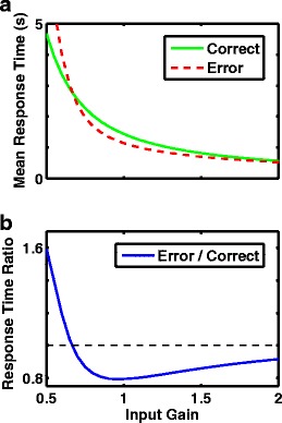
In an attractor model with urgency gating, gain modulation can reproduce the observed shift from slower to faster errors as response time decreases. a Mean response times on error trials and correct trials both decrease as input gain increases in an attractor model (b = 2) with low noise (D = 100Hz ² s ⁻¹) and an urgency gating signal (G _U(t) = t/15). b Ratio of mean error response times to correct response times for the parameters of (a). a–b No time limit was used for these simulations, so threshold was always reached

A curious and related phenomenon arises when strong nonlinearity is combined with a strong urgency-gating signal. In such cases the probability of producing a “slow” error could become greater than the probability of producing a correct response. Because of this, performance of the nonlinear model worsens with increased stimulus duration. In such a regime, the optimal strategy requires switching responses—as has been observed to occur in paradigms sensitive to when a subject deliberately changes his/her mind (Resulaj et al. 2009)—if threshold is not yet reached by the time when the probability distributions for correct and error responses cross over.

Stimulus reversal

If the strong stimulus is reversed at the midpoint of the total stimulus presentation (Fig. 13a) during a situation in which the presentation intervals are short, our simulations using nonlinear models predicts a range of stimulus duration for which the second, reversed stimulus should dominate (Fig. 13c) the decision process, with increasing dominance as the total presentation time increases. This effect has been observed in behavioral data and termed paradoxical integration (Rüter et al. 2012), for the reason that it is not reproducible in a standard, perfect integrator.

Fig. 13.

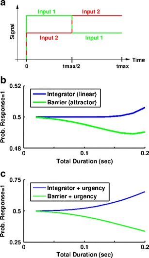
Double-stimulus protocol can favor second stimulus in attractor systems. a In the protocol, the sign of stimulus bias is reversed at the midpoint (tmax/2) of the total duration (tmax), which can vary. b With no urgency-gating signal, G _U(t) = 0, the attractor model produces a small bias toward the second stimulus. The bias increases with total stimulus duration for small durations. Blue dashed curve = perfect integrator, b = 0. Green solid curve = triple attractor with b = 11. For both curves D = 400Hz ² s ⁻¹ (corresponding to2Hz spontaneous activity). c With an urgency-gating signal, G _U(t) = 240 t, responses become more likely as time progresses, so for the triple attractor model (green, b = 25) the second stimulus strongly dominates the response, as seen in behavioral data (Silver et al. 2012). The linear, integrator model retains dominance of the first stimulus (unlike behavioral data). Blue dashed curve = perfect integrator, b = 0. Green solid curve = triple attractor with b = 25. For both curves D = 100Hz ² s ⁻¹. b-c Inputs were strong enough for these simulations that threshold was always reached

An attractor system with an urgency-gating signal reproduces this effect naturally (Fig. 13c), as responses can be dominated by the later signal when any barrier is lower or the initial state is rendered unstable. Paradoxical integration can also occasionally arise in an attractor system with barriers and no urgency-gating signal (Fig. 13b), because errors are relatively fast in a barrier system, such that incorrect responses during the first stimulus (which favor the second stimulus) occur relatively frequently. However, the conditions under which our single-stage system (with or without urgency-gating) emphasizes the second stimulus over the first are not conditions under which the first stimulus alone produces high response accuracy. Thus, while an attractor-based model can explain more of the data than a single integrator, the two-stage model suggested by others (Rüter et al. 2012) remains essential to explain the full range of consecutive-stimulus data. In the two-stage model, a first circuit receives direct stimulus-dependent inputs during stimulus presentation, while a second circuit, which implements the drift-diffusion model (Ratcliff 1978) receives inputs, commencing at stimulus offset, from the buffered final activity of the first circuit. It is noteworthy that in the proposed two-stage decision-making system, the first stage must be an attractor-based “leaky integrator” rather than a perfect integrator (Rüter et al. 2012).

Bimodal response time distributions in a compelled response task reproduced by a non-integrator

An interesting result that can be used to further test our competing models of decision making is the bimodality in the distribution of correct response times observed in vivo in a compelled saccade task (Salinas et al. 2010; Shankar et al. 2011). In this task, a signal cues the monkey to make its response even before the stimulus information became available. We simulate such a protocol with a two-variable model, by commencing the diffusion process (and any urgency-gating signal if present) before adding the bias term favoring a particular response (Fig. 14a).

Fig. 14.

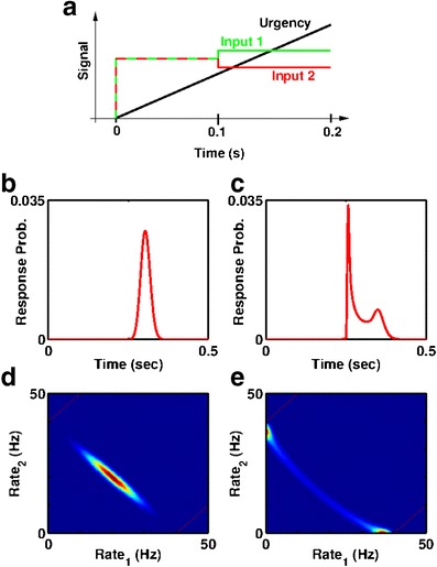
Nonlinear model with an urgency-gating signal reproduces bimodal response distributions in a compelled saccade task in the 2D system. a In the task, the “Go” signal appears (at t = 0) before any input bias (from t = 0.1 s to t = 0.2 s). b, d Results for a perfect integrator (linear model). c, e Results for a nonlinear, attractor model with an urgency-gating signal. b–c Distribution of threshold-crossing times for correct responses. d−e The probability distribution at the mid-point of the task, immediately preceding input bias. b–e Inputs were strong enough for these simulations that threshold was always reached

It proved difficult (though not impossible) to produce this sort of bimodal distribution of response times using a tuned linear system as a perfect integrator; such a system necessarily produces a unimodal probability distribution of firing rates. That is, given $\frac{d{r}_D}{\mathit{dt}}=I_D\left(t\right)+\mathit{D\eta }\left(t\right)$, the solution of the Fokker-Planck equation is $P\left(r_D,t\right)=\frac{1}{\sqrt{2\mathit{\pi Dt}}}exp\left\{-\frac{{\left[r_D-〈r_D\left(t\right)〉\right]}^2}{2\mathit{Dt}}\right\}$ where 〈r _D(t)〉 = ∫ ^t ₀ I _D(t ′)dt ′, a unimodal Gaussian. Only when the input to be integrated was scaled in a highly nonlinear manner as a function of time could bimodal response time distributions be observed with a linear model (Broderick et al. 2009); when we added a forcing term to all of our decision-making models, for example, a second peak in response times arose following onset of the forcing current. However, a sigmoidal time-dependence of the input gain (a fairly severe constraint) was essential for this result; without it, all of our simulations with a perfect integrator resulted in unimodal distributions of response times (Fig. 14b).

On the other hand, a nonlinear system naturally produces a bimodal probability distribution (Fig. 14c) once the fixed point at r _D = 0 becomes unstable (Fig. 14e). That is, any time the symmetric input to the system (before any bias is applied) is sufficient to destabilize the symmetric fixed point but insufficient to force a response, the bimodal probability distribution can lead to a bimodal distribution of correct response times. Indeed, Fig. 14c demonstrates that a nonlinear system with an additive urgency-gating signal reliably leads to a bimodal distribution of correct responses.

It is important to distinguish between predictions regarding individual subjects’ distributions of response times and those observed after averaging across subjects. Bimodal group distributions (Simen et al. 2009) can be fit by mixing two different models of decision-making, and it is reasonable to assume that different models would fit behavior of different subjects. However, in the compelled response task considered here (Shankar et al. 2011), the bimodal distribution arose from a series of trials from the same subject. Thus, the only models that can fit the data are those in which a single set of parameters produces such a bimodal distribution—the nonlinear system achieves this with much greater ease than the perfect integrator.

Single-trial electrophysiological data

The basic properties of simulated single-trial firing-rate trajectories differed depending on whether the system was linear or nonlinear, and on whether an urgency-gating signal was present or absent, and thus could also be used to evaluate models. Note, however, that this is only true for single-trial analyses—activity averaged across trials, a la peri-stimulus time histograms, may well provide an unreliable estimate of these single-trial firing properties (see Section 1).

Introducing sufficient nonlinearity in the effective potential reproduced the results of our prior work (Miller and Katz 2010), in that the time for transition from half-threshold to threshold became fast compared to both the mean time to reach half-threshold and the trial-to-trial standard deviation in threshold crossing times (Table 3). That is, firing rates changed suddenly as the system hopped from one attractor to the next—changes that occurred at slightly different times on different trials. By contrast, the linear models produce broader transitions with less variability across onset times than time to make the transition itself—integrative “ramps” of activity.

Table 3.

Summary of single-trial trajectories in 1-D system. The parameters producing greatest accuracy under our standard conditions are found in the rows where both a > 0 and dG _U/dt > 0 In both cases, T ₁ > T ₁₂: the mean time from stimulus onset to half-threshold is significantly greater than the time to complete the transition. The final column is the correlation across trials between (time to reach half-threshold) and T ₁₂ the time from half-threshold to threshold

D(Hz 2 s −1)	a	dG U/dt (s −1)	T 1	T 12	ρ
100	0	0	.75	.78	−.03
100	0	3	.75	.48*	−.20*
100	3	0	1.65	.77*	−.03
100	3	3	1.00	.29*	−.40*
900	0	0	.42	.55	−.04
900	0	3.5	.29	.28	−.24*
900	9	0	.60	.50	.003
900	14	3.5	.58	.37*	−.29*

These differences can be observed in Fig. 15, which compares the average firing-rate trajectories (n = 100 simulated trials) aligned first to stimulus onset (the PSTH, Fig. 15a) and next to the mid-point of the trajectory (Fig. 15b). The linear perfect integrator would appear to possess a steeper slope according to the standard PSTH, but alignment of trials to each trajectory’s midpoint reveals the significantly sharper transition in the model with urgency-gating signal and attractors.

Fig. 15.

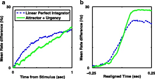
Realignment of trajectories of the difference in firing rate reveals sharper transitions in attractor models. a For each model, mean of 100 correct trajectories of firing-rate difference, r _d(t), aligned to stimulus onset, as in a peri-stimulus time histogram. b Mean of same 100 trajectories for each model, but with each trial realigned to the time its smoothed trajectory reaches 15Hz. a–b Dashed blue curve: linear perfect integrator, b = 0, G _u(t) = 0 (accuracy = 0.708). Solid green curve: more optimal attractor model with urgency-gating, b = 0, G _u(t) = 5 t (accuracy = 0.738)

An urgency-gating signal in particular enhanced the “jumpiness” of single-trial firing trajectories in trials with late decisions, because trials in which responses are later are those with a stronger urgency-gating input, which forces a faster shift of rates toward threshold, at the time of response. These trends were more noticeable in simulations of the low-noise system with D = 100Hz ² s ⁻¹ (Table 3) as noise fluctuations dominated individual trajectories with higher levels of noise.

In summary, neurons in nonlinear attractor networks tend to jump suddenly from one firing rate to another at times that are controlled by system noise (and thus differ from trial to trial), whereas neurons in a perfect integrator produce smoothly ramping firing rate trajectories. Across-trial averages of these processes may well be similar, and “jumpiness” of single-trial, single-neuron spike trains is notoriously difficult to analyze; thus, relating the results of these models to real data requires the simultaneous collection of multiple spike trains, which in attractor models jump in synchrony. There have been few such examinations thus far, but most of those that have been presented suggest either sudden coherent jumps (Seidemann et al. 1996; Jones et al. 2007; Ponce-Alvarez et al. 2012) or combinations of jumps and ramps (Bollimunta et al. 2012).

Discussion

The motivation for the analyses that we have presented is three-fold. First, there is ample justification in the literature (see references in Section 1) to doubt that a perfect integrator is optimal (or even desirable) for decision-making in neural circuitry under realistic environmental constraints. Second, the necessity of fine-tuning of parameters to produce a perfect integrator makes it reasonable to ask whether attractor-based models might provide more robust explanations of decision-making. Third, our analyses of neural data in gustatory cortex during taste processing (Jones et al. 2007) suggest that decisions in the taste system may be reached via “jumps” between multi-neuronal attractor states rather than via continuously varying “ramps” that are produced by an integrator.

Our results suggest that given environmental and neural constraints, perfect integrators are less accurate and less robust than attractor-based models. Furthermore, we have found attractor models to be more compatible with certain behavioral and electrophysiological data.

Accuracy of decision-making

Under a number of conditions, a perfect integrator proves to be less optimal for producing two-alternative forced choice decisions than a system based on transitions between attractors. The simplest such system—three attractors, one for an initial undecided state and one for each of the two decision states—performs better under two general conditions. First, if the mean time to threshold is much shorter than a fixed response time—such as when the system is particularly noisy—the incorporation of barriers to diffusion within the attractor-based model slows down the random walk such that the actual input bias plays a stronger role in decision-making process than it does in the perfect integrator model. Alternatively, in the absence of a time limit for responses, when optimality is measured by maximum reward rate, then attractor-based models can perform better than a perfect integrator if the inter-trial interval is much longer than mean response times.

Furthermore, within the fixed response time paradigm, model mechanisms for ensuring timely responses, such as the inclusion of a forcing or an urgency-gating signal—an addition that is directly supported by psychophysical (Cisek et al. 2009) and electrophysiological (Leon and Shadlen 2003; Janssen and Shadlen 2005; Genovesio et al. 2006; Mita et al. 2009; Churchland et al. 2011) evidence—further improves the advantage of the nonlinear system over a perfect integrator. Although the forcing or urgency-gating signal, here implemented as a temporal jump or ramping of non-specific input, served to destabilize the baseline undecided attractor state, under most conditions the majority of responses were made before such destabilization was complete. Similar effects have been observed when an adaptation current was added to a model of perceptual bistability (Moreno-Bote et al. 2007; Theodoni et al. 2011a; Theodoni et al. 2011b). Thus, in many cases, the trajectories of neural activity under parameters producing greatest accuracy correspond more to one of a stochastic jump between discrete attractor states, than the gradual ramping produced within a perfect integrator (Table 3).

For all of the simulations presented here, the external input signal (the bias, or stimulus strength) remained fixed at a single value. Our results generalize to other input signals, however, because each system is mathematically identical to an alternative system whose inputs, threshold and standard deviation of noise are all scaled by the same multiplicative factor (assuming the attractor/barrier is also appropriately scaled, see Methods). Similarly, our results are not confined to a unique stimulus duration, because a system whose noise variance, barrier height and stimulus strength are scaled by the same multiplicative factor, remains mathematically identical if the stimulus duration is divided by that factor. Thus, ubiquitously, we find that if all parameters are fixed except one, then by adjusting that parameter so as to speed up responses, a crossover is reached after which an attractor-based model is more accurate than a perfect integrator. For example, in all systems—even those with low noise or high threshold, which favor the perfect integrator—a sufficiently strong stimulus bias can always causes the accuracy of the perfect integrator to be bested by the nonlinear model. This is a direct consequence of the attractor model reducing the probability of an incorrect response: the accuracy of attractor models is limited by the slowing of correct responses to produce more undecided trials; if mean response time is sufficiently fast compared to stimulus duration, such limitation is avoided. As a consequence, even without an urgency-gating signal, for any fixed set of conditions—signal strength, noise level, threshold value—for very long stimulus durations, any sufficiently stable attractor model is more accurate than a perfect integrator.

Our results do not in any way contradict well-established theories demonstrating the optimality of the integrator under particular conditions. When there is no time limit for a free response, for instance, a perfect integrator is more accurate for any given mean response time. Furthermore, even in the more realistic situation of fixed stimulus duration, an unbounded integrator is more accurate if the decision is determined by the response bias (i.e., the difference in firing rates between neural pools) at any time in the stimulus period (Wald and Wolfowitz 1948). Equivalently, if inputs can be scaled without changing the signal-to-noise ratio—i. e. assuming no internal noise—then the optimal accuracy for the perfect integrator is highest for any fixed duration. These conditions underlie the bulk of models studied, and so underlie the suggestion that an integrator is universally optimal.

Our study includes multiple conditions, and, we believe, takes into account several important constraints found in nature. First, environmental stimuli can have limited duration, and the time available for making a response may be limited. While using mean response time as a measure of optimality assumes that each additional moment of delay is equally detrimental, we also consider the opposite case, where additional delay beyond a fixed interval is highly detrimental, as responses must be made within a given, fixed duration. Second, the range of integration is limited by the bounds on neural firing rates (Zhang and Bogacz 2010). Third, the neural circuit performing the integration of noisy evidence contributes its own noise. Note that the capabilities of the perfect integrator are limited by the combination of these last two conditions—noise within the circuit causes random variability in neural spiking, which is finite compared to the bounded range of firing rates. Without such internal noise, inputs can always be scaled (by appropriate synaptic strengths) such that for a given input signal-to-noise ratio the integrator fairs best (Fig. 4e). However, given such constraints, the perfect integrator is rarely the optimal system in terms of rate of reward accumulation even in the absence of a time limit for response (Fig. 9). Long intertrial intervals favor attractor models with a barrier (and corresponding higher accuracy but slower responses) while short intertrial intervals favor systems with an unstable initial state upon stimulus onset (cf (Wang 2002)).

Readout of trials that do not reach threshold

One possible shortcoming of the simplest formulation of our model was the presence of “undecided” trials—trials in which the decision variable had not reached either threshold by the requisite response time. While in reality this “problem” affected the attractor model with its barriers to integration more than it did the perfect integrator, the balance of the Results section largely consisted of a consideration a number of possible methods for resolving such situations. At one extreme, that of lowest accuracy (Fig. 2), we assumed subjects would choose to guess a response without bias, if at the end of the decision period threshold was not reached. Such guessing could arise if the signal was too weak, or the limited response time too short, to allow a reliable percept to form. Even this scheme, which was relatively disadvantageous for the attractor-based models, led to fewer accurate decisions for the perfect integrator (Figs. 2 and 4).

At the other extreme, that of maximum accuracy, we simply read out mathematically the sign of the decision variable at the required response time for such “undecided” trials. Such perfect readout further favored the attractor models, increasing their advantage over the perfect integrator (Figs. 2a and 4d). However, since such perfect readout is unlikely in a biological setting, we validated our conclusions by assessing the consequences of other more realistic methods—in particular, a sudden, strong “forcing current” at decision time, or alternatively several variants of urgency-gating signal—for ensuring responses were timely.

Thus, in a subset of analyses, an added urgency-gating signal, which linearly ramps across the stimulus-decision interval (Ditterich 2006), improved the advantage of the nonlinear model. Ramping peri-stimulus time histograms, as observed in several cortical areas of primates (Romo et al. 1999; Brody et al. 2003; Janssen and Shadlen 2005; Genovesio et al. 2006; Mita et al. 2009; Jun et al. 2010), could provide the biological substrate for such a signal. The urgency-gating signal acts as an external control signal to the circuit, shifting its fixed points and thus its function. Such shifts may arise from the stimulus inputs themselves (Wong and Wang 2006; Wong et al. 2007) or from an external switching signal (Machens et al. 2005).

The urgency-gating signal can affect the decision-making process in a number of ways, depending on the nature of the signal and on the readout mechanism. First, the signal could provide a multiplicative gain modulation on the inputs, or an additive unbiased input current. Second, the decision can be made when the difference in firing rates between two populations of cells reaches a threshold or when a single population’s firing rate reaches threshold. Effects were almost identical, except in one case to be described in the following paragraph. In all cases, the improvement in accuracy of the attractor-based model by reducing undecided trials led to it besting the perfect integrator.

With an additive urgency-gating signal, the sum of the population-average firing rates of the two decision-making pools increases for all types of circuits, but only for an attractor-based model does the difference in firing rates also increase. Thus, if a behavioral response is based on a difference in firing rates, the urgency-gating signal does not affect the linear integrator (Fig. 11c, dashed blue curve is identical to Fig. 11a, dashed blue curve). Beyond demonstrating such a difference between attractors and perfect integrators in Fig. 11b, we do not consider or include this difference in other comparisons of their performance. Rather, in 1D models, we either add a destabilizing term (Fig. 5, green dot-dashed trace and Fig. 6a–c) to gradually increase any difference in firing rates in all models (the process that automatically arises in nonlinear 2D models) or we monotonically decrease the response threshold, to represent the rates of individual populations being pushed toward fixed boundaries (Fig. 5, red dashed trace and Fig. 6d–f). Our results did not depend on the precise mechanism—in all cases the attractor-based model bested the perfect integrator.

While the ramping signal appears similar to the output of an integrator, it does not require an integrator, as the signal is independent of any stimulus properties and need have no specific temporal dependence, so long as it is monotonic. Indeed, the ramping of the urgency-gating signal could—just like the apparent ramping of activity in the decision-making circuitry—arise from step-like changes of activity on individual trials (Okamoto et al. 2007; Miller and Katz 2010), so we also simulated the urgency-gating signal as a step change of unbiased input current.

Step-like urgency-gating signals in attractor models increased accuracy to levels above those generated by such signals in the perfect integrator—in fact, an appropriately timed and sized step-input, such as this sort of urgency gate, could always, when combined with an attractor, produce greater accuracy than a ramping urgency gate (data not shown). Such step-like urgency-gating signals are equivalent to our use of a forcing signal to ensure a response, but were lower strength and with randomly-varying onset times. The random variability in timing would lead to the appearance of a gradual ramp of the inputs upon averaging across trials. Recordings from cells providing such an urgency-gating signal would be needed to determine whether the input is ramping or jumping on a trial-by-trial basis.

Comparison with integrator models

Many models incorporating a nonlinearity related to the firing rate responses of neurons serve as perfect integrators only when the total stimulus input dwells in a narrow range, because the quadratic term in an effective potential needs to be precisely canceled by the total input current (e.g. to set the term linear in r _D to zero in Eq. (20)); this is true for most line attractor models, all of which can be integrators (Seung 1996; Seung et al. 2000; Wang 2002; Miller et al. 2003). Such fine tuning of parameters is less essential in model integrators based on the position of an activity “bump” in ring-attractors (Zhang 1996; Compte et al. 2000; Song and Wang 2005) where an approximate equivalence of the long-term mean firing rates of different cells in the circuit is sufficient to produce the necessary continuum of fixed points (Renart et al. 2003). Indeed, near perfect integration has been demonstrated in such a spiking-neuron model circuit for the encoding of head direction (Song and Wang 2005). However, when ring attractors integrate by such continuous movement of the location of a bump of activity (which does not require fine tuning) they do not actually show the monotonic ramping of neural activity observed in decision-making tasks (Shadlen and Newsome 2001; Roitman and Shadlen 2002), nor is it clear how a signal to be integrated by such a model could perform the necessary reset of the “bump” to a specific, stimulus-independent ring location. A system with stable attractors, meanwhile, requires neither a reset signal nor fine-tuning to produce highly accurate decision-making responses when the baseline attractor remains deterministically stable upon stimulus onset. In fact, our stable attractor models were robust to a wide range of specific input parameters.

An animal’s goal in virtually any task is to maximize reward. Arriving at the optimal strategy with which to do this depends fundamentally on balancing the cost of making errors with the cost of taking more time to respond (Simen et al. 2006; Simen et al. 2009; Balci et al. 2011). Adjusting the optimal speed-accuracy tradeoff by varying the inter-trial interval (Fig. 9) again demonstrates that the perfect integrator is not universally the best decision-making system (Zhang and Bogacz 2010). In sum, and when analyzing systems under different experimental conditions, both unstable and attractor-based models should also be considered.

Comparison with behavioral data

Several behavioral tasks have probed the mechanisms underlying decision-making with a stimulus that changes over the course of the decision interval. For example, if the stimulus favors one response then switches to favor the opposite response, the resulting shift in distribution of response times is, in one experiment, reproduced by both a nonlinear model and a perfect integrator (Wang 2002; Huk and Shadlen 2005; Wong et al. 2007; Cisek et al. 2009) and, in another experiment, reproduced by a nonlinear model with an urgency-gating signal but not by a perfect integrator (Cisek et al. 2009). In a similar task with two successive, opposite stimuli, responses are dominated by the second stimulus and more so with increasing (but equal) stimulus duration (Silver et al. 2012). Again, a perfect integrator does not reproduce such results. Moreover, in compelled response tasks (Shankar et al. 2011), in which the cue for a response precedes any stimulus information, the resulting bimodal distribution of response times is not reproduced by a perfect integrator (unless the input gain changes sharply over time (Broderick et al. 2009)). Yet all of these features can be reproduced in a system with attractors and an urgency-gating signal.

Comparison with electrophysiological data

The stable attractor and perfect integrator models make different predictions regarding single-trial analysis of electrophysiological data. A hallmark of stochastic transitions is the large variability in the time of commencement and completion of a transition compared to the duration of the transition itself. The presence of an urgency-gating signal as a gradually ramping input current, meanwhile (Eqs. (17, 18, 20)), should cause later transitions to be even more rapid than earlier transitions, as seen in Table 3. These predictions are contrary to the behavior of an integrator like the drift-diffusion model with the proposed trial-to-trial variability of input bias.

Electrophysiological analysis is complicated by the fact that spikes of single neurons only poorly represent activity of the network as a whole. In particular, the signature of our results—a rapid jump in neural activity between two levels, rather than a slow ramping—is typically lost and unidentifiable in the noisy fluctuations of inter-spike intervals of a single neuron (though see (Okamoto et al. 2007) for single-neuron data supporting rate jumps). Moreover, the typical approach to electrophysiological analysis—an averaging of data across trials aligned on stimulus onset—specifically obscures the single-trial dynamics that distinguish between perfect integration and attractor-based transitions. Thus, it is almost impossible to test these predictions in single-neuron data. However, the now commonplace measurement of spike trains from multiple neurons simultaneously allows one to use more sophisticated analyses, such as Hidden Markov modeling (Abeles et al. 1995; Gat et al. 1997; Jones et al. 2007), and in general to more easily extract differences in trial-to-trial dynamics of underlying states of network activity. At least in the realm of taste decisions, such analyses demonstrate stochastic state transitions during taste processing—transitions which arguably culminate in a two-alternative decision of palatability (Miller and Katz 2010). Single-trial analysis of neural activity in other decision-making tasks is needed to determine whether perfect integration of evidence or attractor-hopping is the more general method for making choices.

Appendix A: Linear models

The drift-diffusion model is an example of a perfect integrator, which can be related to the activity of two groups of neurons if the decision is based on the difference in firing rates of the two groups, and the input to the drift-diffusion model is the difference in inputs to the two neural groups (termed input bias in this paper). Others have described this connection between two-variable and single-variable models before (Usher and McClelland 2001; Bogacz et al. 2006). In Appendix A, we repeat the substance of these analyses using the formalism in this paper, as these methods will allow us to map our two-variable model system with nonlinear firing rate curves of neurons into a single-variable effective potential in Appendices B and C.

Requirements for a perfect integrator

If the spiking rate of each neural group, i (i = 1, 2) is given by r _i and the neural dynamics have a natural time constant, τ, then $\tau \frac{d{r}_i}{\mathit{dt}}=-r_i+f\left(I_i^E,I_i^I\right)$ where f(I ^E, I ^I) is the response of the group of cells to excitatory input current, I ^E and inhibitory input current I ^I. In the simplest models, the response can be written as a weighted difference of input currents f (I  ^E, I ^I) = f (I  ^E − αI  ^I) = f (I), so the firing rate response depends on the sum of recurrent excitation, cross-inhibition and applied current as: I _i = W _S g(r _i) − W _x h(r _j) + I ^app_i(i = 1, 2; j ≠ i) where the functions g(r) and h(r) respectively determine the excitatory and inhibitory current as a function of presynaptic firing rate.

The coupled equations for the dynamics of two groups of cells can produce perfect integration of the difference of inputs, if we assume that: (1) the functions g(r) and h(r)are linear (current into a postsynaptic cell is a linear function of presynaptic firing rate); (2) the function f(I) has a linear range (firing rate of cells is linear in their inputs over some range); and (3) W _S and W _x are appropriately chosen (the strengths of connections are tuned).

Deterministic rate equations can produce fixed points, meaning no change of rate occurs when the rates of both neural groups are at the values given by the fixed point. A fixed point can produce a stable or unstable state depending on whether the dynamics lead the rates to change back toward their values at the fixed point or to move further away following a small deviation. Stable states are often termed attractors, because in the vicinity of the fixed point the rates are deterministically driven to approach the fixed point. The strength of this drive, combined with how much the rates must change away from the fixed point to avoid such a drive to return (termed escaping the basin of attraction) determine how strong an input or noise fluctuation must be to cause the system to change from one stable state to another.

In the following, we show how relaxation of the linearity assumption for f(I) leads to a stable state of “indecision” at low total input that becomes unstable with increasing total input. This motivates our use of attractors and our implementation of an urgency-gating signal as a ramping input current throughout this paper.

To produce a perfect integrator, we set g(r) = h(r) = r and assume f(I) is piece-wise linear:

$$f\left(I\right)=\left\{\begin{array}{c}\hfill 0\mathit{if}I\le 0\hfill \\ \hfill I\frac{r^M}{I^M}\mathit{if}0<I<I^M\hfill \\ \hfill r^M\mathit{if}I\ge I^M\hfill \end{array}\right.$$ 5

where r ^M is the maximum firing rate and I ^M is the input current that produces maximal firing.

We define the sum and difference of the rates of the two cell-groups as r _S = r ₁ + r ₂, r _D = r ₁ − r ₂ and the sum and difference of their inputs as I _S = I ^app_i + I ^app₂, I _D = I ^app_i − I ^app₂.

Thus we can solve the coupled equations:

$$\begin{array}{l}\tau \frac{d{r}_1}{\mathit{dt}}=-r_1+f\left(W_{S}g\left(r_1\right)-W_{x}h\left(r_2\right)+I_1^{\mathit{app}}\right)=-r_1+\left(W_S{r}_1-W_x{r}_2+\frac{I_S+I_D}{2}\right)\frac{r^M}{I^M}\hfill \\ \tau \frac{d{r}_2}{\mathit{dt}}=-r_2+f\left(W_{S}g\left(r_2\right)-W_{x}h\left(r_1\right)+I_2^{\mathit{app}}\right)=-r_2+\left(W_S{r}_2-W_x{r}_1+\frac{I_S-I_D}{2}\right)\frac{r^M}{I^M}\hfill \end{array}$$ 6

to obtain independent dynamics for the sum and differences in rates (Usher and McClelland 2001; Bogacz et al. 2006):

$$\begin{array}{l}\tau \frac{d{r}_S}{\mathit{dt}}=-r_S\left[1-\left(W_S-W_x\right)\frac{r^M}{I^M}\right]+I_S\frac{r^M}{I^M}\hfill \\ \tau \frac{d{r}_D}{\mathit{dt}}=-r_D\left[1-\left(W_S+W_x\right)\frac{r^M}{I^M}\right]+I_D\frac{r^M}{I^M}\hfill \end{array}$$ 7

provided the rates remain in the linear region, such that |r _D| ≤ r ^M and |r _D| ≤ r _s ≤ 2r ^M − |r _D|. In this paper we use τ = 10 ms, on the order of the membrane time constant—a value that is appropriate if synaptic time constants are faster and synaptic input is not dominated by slow NMDA currents (see (Wong and Wang 2006)).

If $\left(W_S+W_x\right)=\frac{I^M}{r^M}$, the difference between the rates of the two groups is directly proportional to the time-integral of the difference in inputs, as shown by many others (Usher and McClelland 2001; Bogacz et al. 2006). In general, if we define a mistuning parameter, $\left.\delta =1-\left(W_S+W_x\right)\frac{r^M}{I^M}\right)$ and set $\epsilon =\left(W_S-W_x\right)\frac{r^M}{I^M}$ then the sum of firing rates converges to the steady state, $r_{{}^S}^{\infty }=\frac{r^M}{1-\epsilon }\frac{I_S}{I^M}$, as the equations simplify:

$$\tau \frac{d{r}_S}{\mathit{dt}}=-r_S\left(1-\epsilon \right)+r^M\frac{I_S}{I^M}$$ 8

and

$$\tau \frac{d{r}_D}{\mathit{dt}}=-\delta r_D+I_D\frac{r^M}{I^M}$$ 9

Under conditions of perfect tuning, such that δ = 0 then Eq. (9) defines a perfect integrator. If δ > 0 then Eq. (9) defines a leaky integrator, as firing rates drift back to zero in the absence of input, and reach a steady state (instead of constantly increasing) with a fixed input bias, I _D. If δ < 0 then Eq. (9) represents an unstable system.

For the model system to produce a binary response, we assume the difference in rates must reach a predetermined positive or negative threshold. Such a threshold must be lower than the steady state summed firing rate, r ^∞_S in these models as perfect integration is lost once any rate drops to zero (as happens once r _D = r _S).

Appendix B: Requirements for an effective potential

If the dynamics of r _D depends only on r _D and not on the sum of rates, r _S (as is true for Eq. (7)) then we can ignore r _S when calculating the result of a decision-making process whose outcome depends only on r _D. In such an event, the system is essentially one-dimensional, allowing the full probability distribution to be solved relatively rapidly—an approach that is more powerful than sampling trajectories one at a time, as it produces precise values for the probability of finding any rate-difference at any given time.

When the system’s relevant dynamics depends only on a single variable, so is one-dimensional (1D), an effective potential (Figs. 1 and 7) can be useful to depict stable points of the system and the relative likelihood of the systems state to move in one direction or another. An effective potential, U(r _D), based on the difference in firing rates, r _D, of two groups of cells can be defined up to an arbitrary constant via:

$$\frac{d{r}_D}{\mathit{dt}}=-\frac{\mathit{dU}\left(r_D\right)}{d{r}_D}$$ 10

The linear system (Eqs. (5, 7–9)) provides a clear example where such an effective potential can be defined, for r _D. In this case (combining Eq. (9) and Eq. (10)) the effective potential is given by:

$$U\left(r_D\right)=\frac{\delta }{2\tau }{r}_D^2-\frac{I_D}{\tau }\frac{r^M}{I^M}{r}_D$$ 11

where $\delta =1-\left(W_S+W_x\right)\frac{r^M}{I^M}$ The integrator is leaky if δ > 0, which then produces a positive quadratic term in the effective potential (Usher and McClelland 2001). In our test of robustness (Fig. 11) we vary the recurrent cross-inhibition, W _x, such that if W _x < 0.5 then δ > 0 and the initial state of the linear system is stable, whereas if W _x > 0.5 then δ < 0 and the initial state of the linear system is unstable.

Nonlinear firing rate curves

Firing rate curves of neurons are rarely linear, or piece-wise linear. In the following two subsections we explore how nonlinearity of neural responses affects the single-variable description of the decision-making process. We first describe general conditions whereby a nonlinear firing rate curve for the neurons can still lead to a single-variable model and an effective potential. We then describe the results when a quadratic term is added and in the final subsection include a cubic term. Of particular interest is how the total input current, I _S, can interact with any nonlinearity in the neural response to alter the shape of the effective potential and how the bias current, I _D, gains multiplicative factors which can strengthen or weaken the input signal as a function of nonlinearity and firing-rate difference, r _D.

The cubic (but not the quadratic) firing rate curve is used for all two-variable model calculations and results in this paper (Fig. 11).

Generalized nonlinear firing rate curves

For more general, nonlinear functions of neural firing rate as a function of inputs, an effective potential for the variable r _D can be produced—i.e. the dynamics of r _D depends only on r _D—if the excitatory self-coupling and inhibitory cross-coupling strengths are balanced to each pool such that ε = (W _S − W _x) = 0. Such a balance is unlikely in practice, but necessary, given the biological reality of nonlinear neural responses, to produce a single variable model, such as the commonly used drift diffusion model (Ratcliff 1978) or any other single-variable model (Eckhoff et al. 2008; Zhang et al. 2009; Zhou et al. 2009; Zhang and Bogacz 2010). If such a balance can be assumed then:

$$\begin{array}{l}\tau \frac{d{r}_1}{\mathit{dt}}=-r_1+F\left(r_1-r_2;I_S+I_D\right)\hfill \\ \tau \frac{d{r}_2}{\mathit{dt}}=-r_2+F\left(r_2-r_1;I_S-I_D\right)\hfill \end{array}$$ 12

in which case, a Taylor expansion of the general nonlinear function, F(Δr; I ^app) about F(0; I _S) leads to:

$$\begin{array}{c}\hfill \tau \frac{d{r}_S}{\mathit{dt}}=-r_S+2F\left(0;I_S\right)+2{\displaystyle {\sum }_{n=1}^{\infty }\frac{1}{\left(2n\right)!}{\displaystyle {\sum }_{r=0}^{2n}{C}_r^{2n}{r}_D^{2n-r}{I}_D^r\frac{{\partial }^{2n}F}{\partial r_D^{2n-r}\partial I_D^r}}}\hfill \\ \hfill \tau \frac{d{r}_D}{\mathit{dt}}=I_D\frac{\partial F}{\partial I_D}-r_D\left(1-2\frac{\partial F}{\partial r_D}\right)+2{\displaystyle {\sum }_{n=1}^{\infty }\frac{1}{\left(2n+1\right)!}{\displaystyle {\sum }_{r=0}^{2n+1}{C}_r^{2n+1}{r}_D^{2n+1-r}{I}_D^r\frac{{\partial }^{2n+1}F}{\partial r_D^{2n+1-r}\partial I_D^r}}}\hfill \end{array}$$ 13

where all derivatives of F are calculated at F(0; I _S). Note that the dynamics for the difference in rates, r _D, are independent of r _S (as they are for the linear model, Eq. (7)) so can be described by a single-variable (1D) model. Such a 1D model can be represented by an effective potential, U(r _D), defined via Eq. (10) $\left(\frac{\mathit{dU}\left(r_D\right)}{d{r}_D}=-\frac{d{r}_D}{\mathit{dt}}\right)$. In the absence of a bias current (i.e. if I _D = 0) we see from Eq. (13) that $\frac{d{r}_S}{\mathit{dt}}$ depends on even powers of r _D whereas $\frac{d{r}_D}{\mathit{dt}}$ depends on odd powers of r _D. The latter result means that the effective potential, U(r _D) is a series of even powers in r _D (so symmetric about the origin) in the absence of bias current. For the simulations within this paper, we include the first three terms in such a series (a quadratic, a quartic and a sextic term), to allow the baseline potential to have up to three attractor states.

Quadratic firing rate curve

We can relax the assumption of linearity of the firing-rate curve, by adding a quadratic term, such that

$$f\left(I\right)=\left\{\begin{array}{cc}0\hfill & \hfill \mathit{if}I\le 0\hfill \\ \hfill I\frac{r^M}{I^M}\left[1+a\frac{I-I^M}{I^M}\right]\hfill & \hfill \mathit{if}0<I<I^M\hfill \\ r^M\hfill & \hfill \mathit{if}I\ge I^M\hfill \end{array}\right.$$ 14

where 0 ≤ a ≤ 1. A quadratic term is the simplest form of nonlinearity, so we include it here to demonstrate the impact of nonlinearity in the cleanest manner, before progressing to inclusion of a cubic term—which allows the firing rate to rise from a baseline of zero and to saturate without discontinuity in its derivative—in the next subsection.

With W _S = W _x (i.e. ε = 0) and $\delta =1-\left(W_S+W_x\right)\frac{r^M}{I^M}$ the dynamics of the sum of rates of the two pools depends on both sum and differences in rates:

$$\tau \frac{d{r}_S}{\mathit{dt}}=-r_S+r^M\frac{I_S}{I^M}\left(1-a\right)+a{r}^M\frac{I_S^2+I_D^2}{2{\left(I^M\right)}^2}+a{r}_D\frac{I_D}{I^M}+a\frac{r_D^2}{2r^M}{\left(1-\delta \right)}^2$$ 15

producing a steady state summed rate that according to the final term increases with the difference in rates and according to the fourth term increases more for correct decisions whereby the product of r _D and I _D is positive.

However, the dynamics for the difference in rates does not depend on the sum of rates:

$$\tau \frac{d{r}_D}{\mathit{dt}}=r^M\frac{I_D}{I^M}\left(1-a\frac{I^M-I_S}{I^M}\right)-r_D\left[\delta +\left(1-\delta \right)a\left(\frac{I^M-I_S}{I^M}\right)\right]$$ 16

The latter result allows us to follow the dynamics of a single variable, the difference in firing rates, r _D and to produce an effective potential, U(r _D) such that $\frac{d{r}_D}{\mathit{dt}}=-\frac{\mathit{dU}\left(r_D\right)}{d{r}_D}$ (see previous section). In the absence of any nonlinearity in the firing-rate curves (α = 0) and with perfect tuning of feedback weights (δ = 0) the effective potential is linear, with a slope proportional to the difference in applied currents (the bias). Adding a quadratic term to the firing-rate curve (0 < α ≤ 1) or imperfect tuning (0 < δ ≤ 1) leads to a quadratic potential, with a point attractor at in the absence of input. If the input is weak, the system maintains an attractor (stable fixed point) near the origin, but given sufficient input (if $I_S>I^M\left[1+\frac{\delta }{\left(1-\delta \right)a}\right]$) the fixed point becomes unstable as the curvature of the potential changes sign. We note that the nonlinear system can produce perfect integration of the difference in inputs if the total input is adjusted precisely such that $I_S=I^M\left[1+\frac{\delta }{\left(1-\delta \right)a}\right]$, in which case rate of change of r _D is again proportional to I _D.

It is worthwhile noting that nonlinearity in the system causes a scaling in the integration term for the input bias, I _D In particular, if the summed current to the system, I _S, ramps up over time then the effect of an unchanging input bias, I _D, increases multiplicatively over time. As shown by Wong and others (Wong et al. 2007; Zhou et al. 2009), this suggests one possible implementation of the suggested gain-modulating urgency-gating signal (Cisek et al. 2009) is a simple monotonic increase of unbiased input to a nonlinear decision-making circuit.

Cubic firing rate curve

If we add a cubic term to the firing rate curve (Fig. 10a) we can in principle remove all discontinuities in it (by setting α = 1 in the following equation):

$$f\left(I\right)=\left\{\begin{array}{ll}0\hfill & \mathit{if}I\le 0\hfill \\ \left(1-a\right)r^M\frac{I}{I^M}+a{r}^M\left[3{\left(\frac{I}{I^M}\right)}^2-2{\left(\frac{I}{I^M}\right)}^3\right]\hfill & \mathit{if}0<I<I^M\hfill \\ r^M\hfill & \mathit{if}I\ge I^M\hfill \end{array}\right.$$ 17

In this case, again by setting W _S = W _x (i.e. ε = 0) and setting a linear dependence of postsynaptic input on presynaptic firing rate, the dynamics for the difference in firing rates of two pools is independent of the sum of their rates. The time dependence of the sum of rates, r _S, depends on both r _S and r _D:

$$\begin{array}{l}\tau \frac{d{r}_S}{\mathit{dt}}=-r_S+\left(1-a\right)r^M\frac{I_S}{I^M}+\frac{3a{r}^M}{2}\left\{{\left(\frac{I_S}{I^M}\right)}^2+{\left[\left(\frac{r_D}{r^M}\right)\left(1-\delta \right)+\frac{I_D}{I^M}\right]}^2\right\}\hfill \\ \begin{array}{cccc}\hfill \hfill & \hfill \hfill & \hfill \hfill & \hfill -\frac{a{r}^M}{2}\left\{{\left(\frac{I_S}{I^M}\right)}^3+3\left(\frac{I_S}{I^M}\right){\left[\left(\frac{r_D}{r^M}\right)\left(1-\delta \right)+\frac{I_D}{I^M}\right]}^2\right\}\hfill \end{array}\hfill \end{array}$$ 18

which can reduce with δ = 0 to:

$$\begin{array}{c}\hfill \tau \frac{d{r}_S}{\mathit{dt}}=-r_S+\left(1-a\right)r^M\frac{I_S}{I^M}+\frac{3a{r}^M}{2}\left\{{\left(\frac{I_S}{I^M}\right)}^2+{\left[\left(\frac{r_D}{r^M}\right)+\frac{I_D}{I^M}\right]}^2\right\}\hfill \\ \hfill -\frac{a{r}^M}{2}\left\{{\left(\frac{I_S}{I^M}\right)}^3+3\left(\frac{I_S}{I^M}\right){\left[\left(\frac{r_D}{r^M}\right)+\frac{I_D}{I^M}\right]}^2\right\}.\hfill \end{array}$$ 19

The dynamics of the rate-difference, r _D, is independent of r _S and follows:

$$\begin{array}{c}\hfill \tau \frac{d{r}_D}{\mathit{dt}}=r^M\frac{I_D}{I^M}\left[1-a+3a\frac{I_S}{I^M}-a\frac{3I_S^2+I_D^2}{2{\left(I^M\right)}^2}\right]\hfill \\ \hfill -r_D\left(\delta +a\left(1-\delta \right)\left[1-3\frac{I_S}{I^M}+3\frac{I_S^2+I_D^2}{2{\left(I^M\right)}^2}\right]\right)\hfill \\ \hfill -3a{\left(1-\delta \right)}^2\frac{r_D^2}{2r^M}\frac{I_D}{I^M}-\frac{a}{2}{\left(1-\delta \right)}^3\frac{r_D^3}{{\left(r^M\right)}^2}\hfill \end{array}$$ 20

which is clearly independent of r _S, allowing us to again write an effective potential for the dynamics, such that $\frac{d{r}_D}{\mathit{dt}}=-\frac{\mathit{dU}\left(r_D\right)}{d{r}_D}$ If the system is tuned such that δ = 0 then the dynamics simplify to produce:

$$\begin{array}{c}\hfill \tau \frac{d{r}_D}{\mathit{dt}}=r^M\frac{I_D}{I^M}\left[1-a+3a\frac{I_S}{I^M}-a\frac{3I_S^2+I_D^2}{2{\left(I^M\right)}^2}\right]\hfill \\ \hfill -a{r}_D\left(1-3\frac{I_S}{I^M}+\frac{3I_S^2+3I_D^2}{2{\left(I^M\right)}^2}\right)-3a\frac{r_D^2}{2r^M}\frac{I_D}{I^M}-\frac{a}{2}\frac{r_D^3}{{\left(r^M\right)}^2}\hfill \end{array}$$ 21

corresponding to an effective potential of

$$\begin{array}{c}\hfill U\left(r_D\right)=-r_D\frac{r^M}{\tau }\frac{I_D}{I^M}\left[1-a+3a\frac{I_S}{I^M}-a\frac{3I_S^2+I_D^2}{2{\left(I^M\right)}^2}\right]\hfill \\ \hfill +r_D^2\frac{a}{2\tau }\left(1-3\frac{I_S}{I^M}+\frac{3I_S^2+3I_D^2}{2{\left(I^M\right)}^2}\right)+r_D^3\frac{a}{2\tau r^M}\frac{I_D}{I^M}+r_D^4\frac{a}{8\tau {\left(r^M\right)}^2}.\hfill \end{array}$$ 22

It is worth noting that any bias, I _D as well as contributing to a linear term in the effective potential acts to stabilize the undecided state via its multiplicative increase of the quadratic term of the potential, while reducing the effect of the bias via a cubic term of the potential. As is the case with a quadratic firing rate curve, the total current, I _S, if large enough is able to destabilize an otherwise stable initial state, while appropriate choice of I _S can cause the quadratic term in the potential to vanish, so that for small r _D the system behaves similarly to a perfect integrator. However, in general, perfect integration is never achieved with a cubic firing rate curve, as the effective potential always contains a quartic component (and a cubic component in the presence of a stimulus bias). Thus, in our formulation with a sextic potential, we allow any quadratic term to be able to vanish upon stimulus onset, but not any higher order terms in the potential.

Appendix C: Effective potential formalism

These analyses of simple systems motivate our simulations of a single-variable (1D) system in two ways. First, they suggest that it is reasonable to extend a decision-making system based on an integrator into one based on a leaky integrator, as in the absence of input the difference in rates follows $\tau \frac{d{r}_D}{\mathit{dt}}=-b{r}_D$ An Ornstein-Uhlenbeck process results from the inclusion of noise in the system. Such a process has been investigated in the context of two-alternative forced choice decision-making and shown in some circumstances to perform better than a perfect integrator (Eckhoff et al. 2008; Zhou et al. 2009; Zhang and Bogacz 2010). Second, the above analyses suggest those features of neural circuits that cause nonlinearities in an effective potential also determine how applied currents alter the dynamics of the system. This allows us to modify the effective potential in the presence of stimulus inputs in a manner that depends on the pre-stimulus nonlinearity.

Since, in the absence of input a decision-making system can possess three attractor states, our pre-stimulus potential used in the majority of 1D calculations is sextic:

$$U\left(r_D,t\right)=b\left(r_D^2-\beta r_D^4+\gamma r_D^6\right)$$ 23

where b, β and γ are parameters defining the structure of the network. Specifically, b, scales the nonlinearity, increasing heights of barriers and depths of attractors, scaling inversely with the times constant for deterministic rate changes. The coefficients of the higher order terms in the potential, β and γ, determine the location of the unstable fixed points (the points beyond which rates must pass to escape the initial stable state) and the stable fixed points of high rate. That is, with neither input bias (I _D = 0) nor an urgency signal (G _U = 0) the system possesses fixed points (where $\frac{d{e}_D}{\mathit{dt}}=0$ and the potential has a maximum or minimum, $\frac{\mathit{dU}}{d{r}_D}=0$) at r _D = 0 (stable), $r_D^2=\frac{\beta }{2\gamma }-\sqrt{{\left(\frac{\beta }{2\gamma }\right)}^2-\frac{1}{\gamma }}$ (unstable) and $r_D^2=\frac{\beta }{2\gamma }+\sqrt{{\left(\frac{\beta }{2\gamma }\right)}^2-\frac{1}{\gamma }}$ (stable). Note that when the nonlinearity parameter, b, is negative, the stability of all steady states reverse. For our standard parameters, with a choice-threshold set at ±20Hz, we fix the location of attractor states at 0 and ±30Hz and the unstable fixed points at ±17Hz via fixed values of β = 4/900 and γ = β/1200. Our results do not qualitatively depend on these values, so long as the threshold for making a response is not much greater than the highest stable steady state firing rates of the system (i.e. 30Hz with these parameters). Indeed, a quadratic potential (with a single steady state at r _D = 0) produces almost identical results (data not shown). We vary the stability of attractors (i.e. the height of barriers between stable states) through the parameter b, which is zero for a perfect integrator. In our results with a quadratic potential, we vary b, while setting β = γ = 0.

Upon stimulus presentation the potential shifts, in its most general form as:

$$U\left(r_D,t\right)=b\prime \left(r_D^2-\beta r_D^4+\gamma r_D^6\right)-i_D\left(t\right)\left(\xi r_D-\zeta r_D^3\right)-\epsilon i_S\left(t\right)b{r}_D^2-G_U\left(t\right)r_D^2$$ 24

where $i_D\left(t\right)=\frac{I_D\left(t\right)}{I^M}$ is the difference between two stimulus currents (the bias), $i_S\left(t\right)=\frac{I_S\left(t\right)}{I^M}$ is the sum of the two stimulus currents and G _U(t) is a linearly ramping urgency gating signal. A comparison of Eq. (24) with the cubic firing-rate formalism (Eq. (22)) allows us to equate terms, such that $b\prime =\left\{\delta +a\left(1-\delta \right)\left[1+3\frac{I_S^2+I_D^2}{2{\left(I^M\right)}^2}\right]\right\}/\tau$, $\beta =\frac{a{\left(1-\delta \right)}^3}{2{\left(r^M\right)}^2\left[\delta +a\left(1-\delta \right)\right]}$, ε = 3(1 − δ)/(2τI ^M), $\xi =\frac{r^M}{I^M}\left\{1-a\left[1-3\frac{I_S}{I^M}-\frac{3I_S^2+I_D^2}{2{\left(I^M\right)}^2}\right]\right\}/\tau$ and ζ = a(1 − δ)²/2(τI ^M r ^M). Since nonlinearity in the firing rate curve (a) can simultaneously deepen attractor wells by increasing the nonlinearity in the potential (b), while decreasing the effective signal strength through a reduction in the proportionality constant, ξ, we also implemented 1D simulations for which increasing b coincided with decreasing ξ. The parameter ζ is set to zero in most simulations, but can be given non-zero values to assess the effects of the stimulus current on changing the shape of the potential (as suggested by Eqs. (21–22)) beyond the necessary addition of a linear term. With our parameters for the firing rate model, the value of ζ was small (ζ = .05a = .0005b), and its inclusion did not produce any significant changes in the results.

Appendix D: Realistic pre-stimulus noise-induced spontaneous activity

One advantage of the 2-variable (2D) system is that it produces a more realistic description of spontaneous network activity than can be achieved with the 1D system. Since the 1D system—which only represents the difference in rates of two groups—does not take into account the actual firing rate of each group, it also cannot take account of the rate of a cell-group passing zero and becoming negative. Thus the 1D representation is only valid if the sum of firing rates is significantly greater than the typical difference in firing rates. When the sum of the firing rates of the two neural groups is low—as it is in periods of spontaneous firing—the difference in firing rates in the 1D system can easily surpass the sum of rates and render the model non-biophysical. To maintain realism of the model, a hard boundary should be enforced, ensuring that individual firing rates are non-negative, so that the difference of firing rates never exceeds the sum. Such enforcement requires a 2D system. Thus, we begin our investigation of 2-D models with an analysis of spontaneous activity, the variability of which determines the variability in the starting point at the onset of any stimulus processing.

In decision-making models, variability in the starting-point reduces the model’s accuracy by producing a random initial bias in favor of one input or another. In our standard 1D simulations we assume the decision-making process begins from an unbiased starting point, namely a δ-function at the origin. In practice, one might expect an attractor-based system with a fixed point to better constrain the starting point for decision-making, because a perfect integrator accumulates random noise in the interval between stimuli (Larsen and Bogacz 2010). Indeed, a general problem for integrator models is the fact that they necessarily integrate noise, and thereby encounter an ever increasing, indeterminate offset error in the absence of input—a problem handled using a reset at the time of stimulus onset (see (Roitman and Shadlen 2002) for electrophysiological evidence of such a reset). However, if a 1D system possesses an attractor state, the firing rates remain within its vicinity, so no reset is needed (Larsen and Bogacz 2010). We wished to assess the importance of these factors in the 2D model, which can reliably reproduce the variability wrought by spontaneous activity.

Figure 10 shows that in the absence of stimulus, the difference between the 2D linear model (Fig. 10b) and 2D nonlinear model (Fig. 10c) is less distinct than the qualitative difference between an attractor model with no drift and an integrator with noise-induced drift described above. Note, however, that the linear model is only an integrator when firing rates of both cell-groups lie on the linear portion of the piece-wise linear firing rate curve. Because the magnitude of the rate-difference cannot surpass the rate-sum (firing rates cannot be negative) any system with two coupled neural groups can only be an integrator in the range − r _S < r _D < r _S. With insufficient input, the linear system possesses an attractor state of zero firing rates for both cell-groups, just like the nonlinear model.

Figure 1b, c are produced with a noise term of D = 900Hz ² s ⁻¹. The typical firing rates of spontaneous activity depend on the level of noise in the system (here we assume input noise as well as internal noise to be present in the absence of a stimulus). In the linear model, one can solve for the steady-state of the sum of firing rates in the absence of inputs, as diffusion in a quadratic potential with a reflecting boundary at the origin:

$$\tau \frac{d{r}_S}{\mathit{dt}}=-r_S+\mathit{D\eta }\left(t\right)\mathrm{if}\mathrm{and}\mathrm{only}\mathrm{if}0<r_S.$$

The solution yields $P\left(r_S\right)\propto exp\left(-\frac{r_S^2}{\mathit{D\tau }}\right)\mathrm{erf}\left(\frac{r_S}{\sqrt{\mathit{D\tau }}}\right)$. Thus, assuming a time constant of τ = 10 ms in our formalism with noise levels given by D = 100Hz ² s ⁻¹, 900Hz ² s ⁻¹ or 2500Hz ² s ⁻¹, typical levels of spontaneous activity are 1, 3 or 5 Hz respectively (where $〈r_S〉\sim \sqrt{\mathit{D\tau }}$) Thus one can assess whether reasonable levels of the noise term are incorporated into a model of a decision-making system via the levels of noise-driven spontaneous activity so produced.

In practice, results of simulations of the decision-making process starting from the equilibrium probability distribution in the absence of inputs differed little from those simulations starting from a δ-function at the origin. That is, a variation of 1-5Hz in the initial values of the firing rate was too small, compared to either the threshold of 20Hz or the variability in rates produced by noise during stimulus presentation, to significantly impact the decision-making process.

A difference between linear and nonlinear models can be seen in the shapes of the probability distributions in Fig. 10b, c. For the linear model, the difference in firing rates, r _D, has a uniform probability distribution (for a given rate-sum, r _S, it has no preferred value of rate-difference, r _D). This leads to a negative correlation between the firing rates, r ₁ and r ₂, of the two cell-groups in the linear model. By contrast, the difference in rates always peaks at zero for the nonlinear system, which produces near-circular contours of constant probability in the limit a = 1 (Fig. 10c). In such a case, the probability density is approximately proportional to $exp\left(-\frac{r_1^2+r_2^2}{2{\sigma }^2}\right)$ such that the two firing rates are uncorrelated. Thus the nonlinear system can have uncorrelated firing rates between two groups of cells in the absence of input, but a negative correlation between them (as in all decision-making circuits) once input is applied. Such a shift toward more negative cross-correlations after a stimulus is applied is a unique feature of the nonlinear model that in the future could be tested via multi-unit electrophysiological recordings.

References

- Abeles M, Bergman H, Gat I, Meilijson I, Seidemann E, Tishby N, Vaadia E. Cortical activity flips among quasi-stationary states. Proceedings of the National Academy of Sciences of the United States of America. 1995;92:8616–8620. doi: 10.1073/pnas.92.19.8616. [DOI] [PMC free article] [PubMed] [Google Scholar]
- Balci F, Simen P, Niyogi R, Saxe A, Hughes JA, Holmes P, Cohen JD. Acquisition of decision making criteria: reward rate ultimately beats accuracy. Attention, Perception, & Psychophysics. 2011;73:640–657. doi: 10.3758/s13414-010-0049-7. [DOI] [PMC free article] [PubMed] [Google Scholar]
- Beck JM, Ma WJ, Kiani R, Hanks T, Churchland AK, Roitman J, Shadlen MN, Latham PE, Pouget A. Probabilistic population codes for Bayesian decision making. Neuron. 2008;60:1142–1152. doi: 10.1016/j.neuron.2008.09.021. [DOI] [PMC free article] [PubMed] [Google Scholar]
- Bertsekas DP. Dynamic Programming and Optimal Control. Belmont: Athena Scientific; 2005. [Google Scholar]
- Bogacz R, Brown E, Moehlis J, Holmes P, Cohen JD. The physics of optimal decision making: a formal analysis of models of performance in two-alternative forced-choice tasks. Psychological Review. 2006;113:700–765. doi: 10.1037/0033-295X.113.4.700. [DOI] [PubMed] [Google Scholar]
- Bogacz R, Hu PT, Holmes PJ, Cohen JD. Do humans produce the speed-accuracy trade-off that maximizes reward rate? Quarterly Journal of Experimental Psychology. 2010;63:863–891. doi: 10.1080/17470210903091643. [DOI] [PMC free article] [PubMed] [Google Scholar]
- Bollimunta A, Totten D, Ditterich J. Neural dynamics of choice: single-trial analysis of decision-related activity in parietal cortex. The Journal of neuroscience: the official journal of the Society for Neuroscience. 2012;32:12684–12701. doi: 10.1523/JNEUROSCI.5752-11.2012. [DOI] [PMC free article] [PubMed] [Google Scholar]
- Bouvrie, J., Slotine, J.J. (2011). Synchronization and Redundancy: Implications for Robustness of Neural Learning and Decision Making. Neural Computation 23, 2915–2941. [DOI] [PubMed]
- Broderick T, Wong-Lin KF, Holmes P. Closed-form approximations of first-passage distributions for a stochastic decision-making model. Applied Mathematical Research Express. 2009;2009:123–141. doi: 10.1093/amrx/abp008. [DOI] [PMC free article] [PubMed] [Google Scholar]
- Brody CD, Hernández A, Zainos A, Lemus L, Romo R. Timing and neural encoding of somatosensory parametric working memory in macaque prefrontal cortex. Cerebral Cortex. 2003;13:1196–1207. doi: 10.1093/cercor/bhg100. [DOI] [PubMed] [Google Scholar]
- Brown E, Gao J, Holmes P, Bogacz R, Gilzenrat M, Cohen JD. Simple neural networks that optimize decisions. International Journal of Bifurcation and Chaos. 2005;15:803–826. [Google Scholar]
- Churchland AK, Kiani R, Shadlen MN. Decision-making with multiple alternatives. Nature Neuroscience. 2008;11:693–702. doi: 10.1038/nn.2123. [DOI] [PMC free article] [PubMed] [Google Scholar]
- Churchland AK, Kiani R, Chaudhuri R, Wang XJ, Pouget A, Shadlen MN. Variance as a signature of neural computations during decision making. Neuron. 2011;69:818–831. doi: 10.1016/j.neuron.2010.12.037. [DOI] [PMC free article] [PubMed] [Google Scholar]
- Cisek P, Puskas GA, El-Murr S. Decisions in changing conditions: the urgency-gating model. Journal of Neuroscience. 2009;29:11560–11571. doi: 10.1523/JNEUROSCI.1844-09.2009. [DOI] [PMC free article] [PubMed] [Google Scholar]
- Compte A, Brunel N, Goldman-Rakic PS, Wang XJ. Synaptic mechanisms and network dynamics underlying spatial working memory in a cortical network model. Cerebral Cortex. 2000;10:910–923. doi: 10.1093/cercor/10.9.910. [DOI] [PubMed] [Google Scholar]
- Deco G, Marti D. Extended method of moments for deterministic analysis of stochastic multistable neurodynamical systems. Physical Review. E, Statistical, Nonlinear, and Soft Matter Physics. 2007;75:031913. doi: 10.1103/PhysRevE.75.031913. [DOI] [PubMed] [Google Scholar]
- Deco G, Rolls ET. Decision-making and Weber’s law: a neurophysiological model. European Journal of Neuroscience. 2006;24:901–916. doi: 10.1111/j.1460-9568.2006.04940.x. [DOI] [PubMed] [Google Scholar]
- Deco G, Rolls ET, Romo R. Stochastic dynamics as a principle of brain function. Progress in Neurobiology. 2009;88:1–16. doi: 10.1016/j.pneurobio.2009.01.006. [DOI] [PubMed] [Google Scholar]
- Deco, G., Rolls, E. T., Albantakis, L., Romo, R. (2013). Brain mechanisms for perceptual and reward-related decision-making. Progress in Neurobiology, 103, 194–213. [DOI] [PubMed]
- Ditterich J. Evidence for time-variant decision making. The European Journal of Neuroscience. 2006;24:3628–3641. doi: 10.1111/j.1460-9568.2006.05221.x. [DOI] [PubMed] [Google Scholar]
- Drugowitsch J, Moreno-Bote R, Churchland AK, Shadlen MN, Pouget A. The cost of accumulating evidence in perceptual decision making. The Journal of neuroscience: the official journal of the Society for Neuroscience. 2012;32:3612–3628. doi: 10.1523/JNEUROSCI.4010-11.2012. [DOI] [PMC free article] [PubMed] [Google Scholar]
- Eckhoff P, Holmes P, Law C, Connolly PM, Gold JI. On diffusion processes with variable drift rates as models for decision making during learning. New Journal of Physics. 2008;10:nihpa49499. doi: 10.1088/1367-2630/10/1/015006. [DOI] [PMC free article] [PubMed] [Google Scholar]
- Eckhoff P, Wong-Lin KF, Holmes P. Optimality and robustness of a biophysical decision-making model under norepinephrine modulation. The Journal of neuroscience: the official journal of the Society for Neuroscience. 2009;29:4301–4311. doi: 10.1523/JNEUROSCI.5024-08.2009. [DOI] [PMC free article] [PubMed] [Google Scholar]
- Eckhoff P, Wong-Lin K, Holmes P. Dimension reduction and dynamics of a spiking neural network model for decision making under neuromodulation. SIAM Journal on Applied Dynamical Systems. 2011;10:148–188. doi: 10.1137/090770096. [DOI] [PMC free article] [PubMed] [Google Scholar]
- Farkas Z, Fülöp T. One-dimensional drift-diffusion between two absorbing boundaries: application to granular segregation. Journal of Physics AA: Mathematical and General. 2001;34:3191–3198. [Google Scholar]
- Feng S, Holmes P, Rorie A, Newsome WT. Can monkeys choose optimally when faced with noisy stimuli and unequal rewards? PLoS Computational Biology. 2009;5:e1000284. doi: 10.1371/journal.pcbi.1000284. [DOI] [PMC free article] [PubMed] [Google Scholar]
- Frazier, P. I., Yu, A. J. (2007). Sequential hypothesis testing under stochastic deadlines. In J. C. Platt, et al. (Eds.), Advances in Neural Information Processing Systems (NIPS), vol. 20 (p. 953).
- Gammaitoni L, Hänggi P. Stochastic Resonance. Reviews of Modern Physics. 1998;70:223–287. [Google Scholar]
- Gat, I., Tishby, N., Abeles, M. (1997). Hidden markov modeling of simultaneously recorded cells in the associative cortex of behaving monkeys.
- Genovesio A, Tsujimoto S, Wise SP. Neuronal activity related to elapsed time in prefrontal cortex. Journal of Neurophysiology. 2006;95:3281–3285. doi: 10.1152/jn.01011.2005. [DOI] [PMC free article] [PubMed] [Google Scholar]
- Glimcher PW. Making choices: the neurophysiology of visual-saccadic decision making. Trends in Neurosciences. 2001;24:654–659. doi: 10.1016/s0166-2236(00)01932-9. [DOI] [PubMed] [Google Scholar]
- Glimcher PW. The neurobiology of visual-saccadic decision making. Annual Review of Neuroscience. 2003;26:133–179. doi: 10.1146/annurev.neuro.26.010302.081134. [DOI] [PubMed] [Google Scholar]
- Gluckman BJ, So P, Netoff TI, Spano ML, Schiff SJ. Stochastic resonance in mammalian neuronal networks. Chaos. 1998;8:588–598. doi: 10.1063/1.166340. [DOI] [PubMed] [Google Scholar]
- Gold JI, Shadlen MN. Representation of a perceptual decision in developing oculomotor commands. Nature. 2000;404:390–394. doi: 10.1038/35006062. [DOI] [PubMed] [Google Scholar]
- Gold JI, Shadlen MN. Neural computations that underlie decisions about sensory stimuli. Trends in Cognitive Sciences. 2001;5:10–16. doi: 10.1016/s1364-6613(00)01567-9. [DOI] [PubMed] [Google Scholar]
- Gold JI, Shadlen MN. The influence of behavioral context on the representation of a perceptual decision in developing oculomotor commands. The Journal of Neuroscience: the Official Journal of the Society for Neuroscience. 2003;23:632–651. doi: 10.1523/JNEUROSCI.23-02-00632.2003. [DOI] [PMC free article] [PubMed] [Google Scholar]
- Gold JI, Shadlen MN. The neural basis of decision making. Annual Review of Neuroscience. 2007;30:535–574. doi: 10.1146/annurev.neuro.29.051605.113038. [DOI] [PubMed] [Google Scholar]
- Goldman MS, Levine JH, Major G, Tank DW, Seung HS. Robust persistent neural activity in a model integrator with multiple hysteretic dendrites per neuron. Cerebral Cortex. 2003;13:1185–1195. doi: 10.1093/cercor/bhg095. [DOI] [PubMed] [Google Scholar]
- Huk AC, Shadlen MN. Neural activity in macaque parietal cortex reflects temporal integration of visual motion signals during perceptual decision making. The Journal of Neuroscience: the Official Journal of the Society for Neuroscience. 2005;25:10420–10436. doi: 10.1523/JNEUROSCI.4684-04.2005. [DOI] [PMC free article] [PubMed] [Google Scholar]
- Janssen P, Shadlen MN. A representation of the hazard rate of elapsed time in macaque area LIP. Nature Neuroscience. 2005;8:234–241. doi: 10.1038/nn1386. [DOI] [PubMed] [Google Scholar]
- Jones LM, Fontanini A, Sadacca BF, Miller P, Katz DB. Natural stimuli evoke dynamic sequences of states in sensory cortical ensembles. Proceedings of the National Academy of Sciences of the United States of America. 2007;104:18772–18777. doi: 10.1073/pnas.0705546104. [DOI] [PMC free article] [PubMed] [Google Scholar]
- Jun JK, Miller P, Hernandez A, Zainos A, Lemus L, Brody CD, Romo R. Heterogenous population coding of a short-term memory and decision task. The Journal of Neuroscience: the Official Journal of the Society for Neuroscience. 2010;30:916–929. doi: 10.1523/JNEUROSCI.2062-09.2010. [DOI] [PMC free article] [PubMed] [Google Scholar]
- Kiani R, Hanks TD, Shadlen MN. Bounded integration in parietal cortex underlies decisions even when viewing duration is dictated by the environment. The Journal of Neuroscience: the Official Journal of the Society for Neuroscience. 2008;28:3017–3029. doi: 10.1523/JNEUROSCI.4761-07.2008. [DOI] [PMC free article] [PubMed] [Google Scholar]
- Koulakov AA, Raghavachari S, Kepecs A, Lisman JE. Model for a robust neural integrator. Nature Neuroscience. 2002;5:775–782. doi: 10.1038/nn893. [DOI] [PubMed] [Google Scholar]
- Larsen T, Bogacz R. Initiation and termination of integration in a decision process. Neural Networks. 2010;23:322–333. doi: 10.1016/j.neunet.2009.11.015. [DOI] [PubMed] [Google Scholar]
- Leon MI, Shadlen MN. Representation of time by neurons in the posterior parietal cortex of the macaque. Neuron. 2003;38:317–327. doi: 10.1016/s0896-6273(03)00185-5. [DOI] [PubMed] [Google Scholar]
- Lo CC, Wang XJ. Cortico-basal ganglia circuit mechanism for a decision threshold in reaction time tasks. Nature Neuroscience. 2006;9:956–963. doi: 10.1038/nn1722. [DOI] [PubMed] [Google Scholar]
- Luce RD. Response Times. New York: Oxford University Press; 1986. [Google Scholar]
- Luna, R., Hernández, A., Brody, C.D., Romo, R. (2005). Neural codes for perceptual discrimination in primary somatosensory cortex. Nature Neuroscience 8, 1210–1219. [DOI] [PubMed]
- Machens CK, Romo R, Brody CD. Flexible control of mutual inhibition: a neural model of two-interval discrimination. Science. 2005;307:1121–1124. doi: 10.1126/science.1104171. [DOI] [PubMed] [Google Scholar]
- Marti D, Deco G, Mattia M, Gigante G, Del Giudice P. A fluctuation-driven mechanism for slow decision processes in reverberant networks. PLoS One. 2008;3:e2534. doi: 10.1371/journal.pone.0002534. [DOI] [PMC free article] [PubMed] [Google Scholar]
- Mazurek ME, Roitman JD, Ditterich J, Shadlen MN. A role for neural integrators in perceptual decision making. Cerebral Cortex. 2003;13:1257–1269. doi: 10.1093/cercor/bhg097. [DOI] [PubMed] [Google Scholar]
- McDonnell MD, Abbott D. What Is Stochastic Resonance? Definitions, Misconceptions, Debates, and Its Relevance to Biology. PLoS Computational Biology. 2009;5:e1000348. doi: 10.1371/journal.pcbi.1000348. [DOI] [PMC free article] [PubMed] [Google Scholar]
- Meyer-Baese A, Koshkouei AJ, Emmett MR, Goodall DP. Global stability analysis and robust design of multi-time-scale biological networks under parametric uncertainties. Neural Networks: the Official Journal of the International Neural Network Society. 2009;22:658–663. doi: 10.1016/j.neunet.2009.06.051. [DOI] [PubMed] [Google Scholar]
- Miller P, Katz DB. Stochastic transitions between neural states in taste processing and decision-making. Journal of Neuroscience. 2010;30:2559–2570. doi: 10.1523/JNEUROSCI.3047-09.2010. [DOI] [PMC free article] [PubMed] [Google Scholar]
- Miller P, Katz DB. Stochastic Transitions between States of Neural Activity. In: Ding M, Glanzman DL, editors. The Dynamic Brain: An Exploration of Neuronal Variability and Its Functional Significance. New York: Oxford University Press; 2011. pp. 29–46. [Google Scholar]
- Miller P, Brody CD, Romo R, Wang XJ. A recurrent network model of somatosensory parametric working memory in the prefrontal cortex. Cerebral Cortex. 2003;13:1208–1218. doi: 10.1093/cercor/bhg101. [DOI] [PMC free article] [PubMed] [Google Scholar]
- Mita A, Mushiake H, Shima K, Matsuzaka Y, Tanji J. Interval time coding by neurons in the presupplementary and supplementary motor areas. Nature Neuroscience. 2009;12:502–507. doi: 10.1038/nn.2272. [DOI] [PubMed] [Google Scholar]
- Moreno-Bote R, Rinzel J, Rubin N. Noise-induced alternations in an attractor network model of perceptual bistability. Journal of Neurophysiology. 2007;98:1125–1139. doi: 10.1152/jn.00116.2007. [DOI] [PMC free article] [PubMed] [Google Scholar]
- Nigoyi R, Wong-Lin K. Abstract #246 Computational and Systems Neuroscience (CoSyNe) Salt Lake City: Frontiers in Neuroscience; 2010. Time-varying gain modulation on neural circuit dynamics and performance in perceptual decisions. [Google Scholar]
- Okamoto H, Isomura Y, Takada M, Fukai T. Temporal integration by stochastic recurrent network dynamics with bimodal neurons. Journal of Neurophysiology. 2007;97:3859–3867. doi: 10.1152/jn.01100.2006. [DOI] [PubMed] [Google Scholar]
- Platt ML, Glimcher PW. Neural correlates of decision variables in parietal cortex. Nature. 1999;400:233–238. doi: 10.1038/22268. [DOI] [PubMed] [Google Scholar]
- Ponce-Alvarez A, Nacher V, Luna R, Riehle A, Romo R. Dynamics of cortical neuronal ensembles transit from decision making to storage for later report. The Journal of Neuroscience: the Official Journal of the Society for Neuroscience. 2012;32:11956–11969. doi: 10.1523/JNEUROSCI.6176-11.2012. [DOI] [PMC free article] [PubMed] [Google Scholar]
- Purcell BA, Heitz RP, Cohen JY, Schall JD, Logan GD, Palmeri TJ. Neurally constrained modeling of perceptual decision making. Psychological Review. 2010;117:1113–1143. doi: 10.1037/a0020311. [DOI] [PMC free article] [PubMed] [Google Scholar]
- Ratcliff R. A theory of memory retrieval. Psychological Review. 1978;85:59–108. [Google Scholar]
- Ratcliff R. Modeling aging effects on two-choice tasks: response signal and response time data. Psychology and Aging. 2008;23:900–916. doi: 10.1037/a0013930. [DOI] [PMC free article] [PubMed] [Google Scholar]
- Ratcliff R, McKoon G. The diffusion decision model: theory and data for two-choice decision tasks. Neural Computation. 2008;20:873–922. doi: 10.1162/neco.2008.12-06-420. [DOI] [PMC free article] [PubMed] [Google Scholar]
- Ratcliff R, Rouder JN. Modeling response times for two-choice decisions. Psychological Science. 1998;9:347–356. [Google Scholar]
- Ratcliff R, Cherian A, Segraves M. A comparison of macaque behavior and superior colliculus neuronal activity to predictions from models of two-choice decisions. Journal of Neurophysiology. 2003;90:1392–1407. doi: 10.1152/jn.01049.2002. [DOI] [PubMed] [Google Scholar]
- Renart A, Song P, Wang XJ. Robust spatial working memory through homeostatic synaptic scaling in heterogeneous cortical networks. Neuron. 2003;38:473–485. doi: 10.1016/s0896-6273(03)00255-1. [DOI] [PubMed] [Google Scholar]
- Resulaj A, Kiani R, Wolpert DM, Shadlen MN. Changes of mind in decision-making. Nature. 2009;461:263–266. doi: 10.1038/nature08275. [DOI] [PMC free article] [PubMed] [Google Scholar]
- Roitman JD, Shadlen MN. Response of neurons in the lateral intraparietal area during a combined visual discrimination reaction time task. Journal of Neuroscience. 2002;22:9475–9489. doi: 10.1523/JNEUROSCI.22-21-09475.2002. [DOI] [PMC free article] [PubMed] [Google Scholar]
- Romo R, Brody CD, Hernández A, Lemus L. Neuronal correlates of parametric working memory in the prefrontal cortex. Nature. 1999;399:470–474. doi: 10.1038/20939. [DOI] [PubMed] [Google Scholar]
- Romo R, Hernández A, Zainos A, Lemus L, Brody CD. Neuronal correlates of decision-making in secondary somatosensory cortex. Nature Neuroscience. 2002;5:1217–1225. doi: 10.1038/nn950. [DOI] [PubMed] [Google Scholar]
- Romo R, Hernández A, Zainos A. Neuronal correlates of a perceptual decision in ventral premotor cortex. Neuron. 2004;41:165–173. doi: 10.1016/s0896-6273(03)00817-1. [DOI] [PubMed] [Google Scholar]
- Roxin A, Ledberg A. Neurobiological models of two-choice decision making can be reduced to a one-dimensional nonlinear diffusion equation. PLoS Computational Biology. 2008;4:e1000046. doi: 10.1371/journal.pcbi.1000046. [DOI] [PMC free article] [PubMed] [Google Scholar]
- Rüter J, Marcille N, Sprekeler H, Gerstner W, Herzog MH. Paradoxical evidence integration in rapid decision processes. PLoS Computational Biology. 2012;8:e1002382. doi: 10.1371/journal.pcbi.1002382. [DOI] [PMC free article] [PubMed] [Google Scholar]
- Sakai Y, Okamoto H, Fukai T. Computational algorithms and neuronal network models underlying decision processes. Neural Networks. 2006;19:1091–1105. doi: 10.1016/j.neunet.2006.05.034. [DOI] [PubMed] [Google Scholar]
- Salinas E, Shankar S, Costello MG, Zhu D, Stanford TR. Waiting is the Hardest Part: Comparison of Two Computational Strategies for Performing a Compelled-Response Task. Frontiers in Computational Neuroscience. 2010;4:153. doi: 10.3389/fncom.2010.00153. [DOI] [PMC free article] [PubMed] [Google Scholar]
- Seidemann E, Meilijson I, Abeles M, Bergman H, Vaadia E. Simultaneously recorded single units in the frontal cortex go through sequences of discrete and stable states in monkeys performing a delayed localization task. Journal of Neuroscience. 1996;16:752–768. doi: 10.1523/JNEUROSCI.16-02-00752.1996. [DOI] [PMC free article] [PubMed] [Google Scholar]
- Seung HS. How the brain keeps the eyes still. Proceedings of the National Academy of Sciences of the United States of America. 1996;93:13339–13344. doi: 10.1073/pnas.93.23.13339. [DOI] [PMC free article] [PubMed] [Google Scholar]
- Seung HS, Lee DD, Reis BY, Tank DW. The autapse: a simple illustration of short-term analog memory storage by tuned synaptic feedback. Journal of Computational Neuroscience. 2000;9:171–185. doi: 10.1023/a:1008971908649. [DOI] [PubMed] [Google Scholar]
- Shadlen MN, Newsome WT. Motion perception: seeing and deciding. Proceedings of the National Academy of Sciences of the United States of America. 1996;93:628–633. doi: 10.1073/pnas.93.2.628. [DOI] [PMC free article] [PubMed] [Google Scholar]
- Shadlen MN, Newsome WT. Neural basis of a perceptual decision in the parietal cortex (area LIP) of the rhesus monkey. Journal of Neurophysiology. 2001;86:1916–1936. doi: 10.1152/jn.2001.86.4.1916. [DOI] [PubMed] [Google Scholar]
- Shankar S, Massoglia DP, Zhu D, Costello MG, Stanford TR, Salinas E. Tracking the temporal evolution of a perceptual judgment using a compelled-response task. The Journal of Neuroscience: the Official Journal of the Society for Neuroscience. 2011;31:8406–8421. doi: 10.1523/JNEUROSCI.1419-11.2011. [DOI] [PMC free article] [PubMed] [Google Scholar]
- Shea-Brown E, Gilzenrat MS, Cohen JD. Optimization of decision making in multilayer networks: the role of locus coeruleus. Neural Computation. 2008;20:2863–2894. doi: 10.1162/neco.2008.03-07-487. [DOI] [PubMed] [Google Scholar]
- Silver MR, Grossberg S, Bullock D, Histed MH, Miller EK. A neural model of sequential movement planning and control of eye movements: Item-Order-Rank working memory and saccade selection by the supplementary eye fields. Neural Networks: the Official Journal of the International Neural Network Society. 2012;26:29–58. doi: 10.1016/j.neunet.2011.10.004. [DOI] [PubMed] [Google Scholar]
- Simen P, Cohen JD, Holmes P. Rapid decision threshold modulation by reward rate in a neural network. Neural Networks: the Official Journal of the International Neural Network Society. 2006;19:1013–1026. doi: 10.1016/j.neunet.2006.05.038. [DOI] [PMC free article] [PubMed] [Google Scholar]
- Simen P, Contreras D, Buck C, Hu P, Holmes P, Cohen JD. Reward rate optimization in two-alternative decision making: empirical tests of theoretical predictions. Journal of Experimental Psychology. Human Perception and Performance. 2009;35:1865–1897. doi: 10.1037/a0016926. [DOI] [PMC free article] [PubMed] [Google Scholar]
- Smith PL, Ratcliff R. Psychology and neurobiology of simple decisions. Trends in Neurosciences. 2004;27:161–168. doi: 10.1016/j.tins.2004.01.006. [DOI] [PubMed] [Google Scholar]
- Song P, Wang XJ. Angular Path Integration by Moving “Hill of Activity”: A Spiking Neuron Model without Recurrent Excitation of the Head-Direction System. Journal of Neuroscience. 2005;25:1002–1014. doi: 10.1523/JNEUROSCI.4172-04.2005. [DOI] [PMC free article] [PubMed] [Google Scholar]
- Standage D, You H, Wang DH, Dorris MC. Gain modulation by an urgency signal controls the speed-accuracy trade-off in a network model of a cortical decision circuit. Frontiers in Computational Neuroscience. 2011;5:7. doi: 10.3389/fncom.2011.00007. [DOI] [PMC free article] [PubMed] [Google Scholar]
- Stanford TR, Shankar S, Massoglia DP, Costello MG, Salinas E. Perceptual decision making in less than 30 milliseconds. Nature Neuroscience. 2010;13:379–385. doi: 10.1038/nn.2485. [DOI] [PMC free article] [PubMed] [Google Scholar]
- Swensson RG. The elusive tradeoff: speed versus accuracy in visual discrimination tasks. Perception & Psychophysics. 1972;12:16–32. [Google Scholar]
- Theodoni P, Kovacs G, Greenlee MW, Deco G. Neuronal adaptation effects in decision making. Journal of Neuroscience. 2011;31:234–246. doi: 10.1523/JNEUROSCI.2757-10.2011. [DOI] [PMC free article] [PubMed] [Google Scholar]
- Theodoni P, Panagiotaropoulos TI, Kapoor V, Logothetis NK, Deco G. Cortical microcircuit dynamics mediating binocular rivalry: the role of adaptation in inhibition. Frontiers in Human Neuroscience. 2011;5:145. doi: 10.3389/fnhum.2011.00145. [DOI] [PMC free article] [PubMed] [Google Scholar]
- Usher M, McClelland JL. The time course of perceptual choice: the leaky, competing accumulator model. Psychological Review. 2001;108:550–592. doi: 10.1037/0033-295x.108.3.550. [DOI] [PubMed] [Google Scholar]
- Wald A. Sequential analysis. New York: Wiley; 1947. [Google Scholar]
- Wald A, Wolfowitz J. Optimum character of the sequential probability ratio test. Annals of Mathematical Statistics. 1948;19:326–339. [Google Scholar]
- Wang XJ. Synaptic reverberation underlying mnemonic persistent activity. Trends in Neurosciences. 2001;24:455–463. doi: 10.1016/s0166-2236(00)01868-3. [DOI] [PubMed] [Google Scholar]
- Wang XJ. Probabilistic decision making by slow reverberation in cortical circuits. Neuron. 2002;36:955–968. doi: 10.1016/s0896-6273(02)01092-9. [DOI] [PubMed] [Google Scholar]
- Wong KF, Wang XJ. A recurrent network mechanism of time integration in perceptual decisions. The Journal of Neuroscience: the Official Journal of the Society for Neuroscience. 2006;26:1314–1328. doi: 10.1523/JNEUROSCI.3733-05.2006. [DOI] [PMC free article] [PubMed] [Google Scholar]
- Wong KF, Huk AC, Shadlen MN, Wang XJ. Neural circuit dynamics underlying accumulation of time-varying evidence during perceptual decision making. Frontiers in Computational Neuroscience. 2007;1:6. doi: 10.3389/neuro.10.006.2007. [DOI] [PMC free article] [PubMed] [Google Scholar]
- Yoshida T, Katz DB. Control of prestimulus activity related to improved sensory coding within a discrimination task. The Journal of Neuroscience: the Official Journal of the Society for Neuroscience. 2011;31:4101–4112. doi: 10.1523/JNEUROSCI.4380-10.2011. [DOI] [PMC free article] [PubMed] [Google Scholar]
- Zhang K. Representation of spatial orientation by the intrinsic dynamics of the head-direction cell ensemble: a theory. The Journal of Neuroscience: the Official Journal of the Society for Neuroscience. 1996;16:2112–2126. doi: 10.1523/JNEUROSCI.16-06-02112.1996. [DOI] [PMC free article] [PubMed] [Google Scholar]
- Zhang J, Bogacz R. Bounded Ornstein-Uhlenbeck models for two-choice time controlled tasks. Journal of Mathematical Psychology. 2010;54:322–333. doi: 10.1016/j.jmp.2009.03.001. [DOI] [PMC free article] [PubMed] [Google Scholar]
- Zhang J, Bogacz R, Holmes P. A comparison of bounded diffusion models for choice in time controlled tasks. Journal of Mathematical Psychology. 2009;53:231–241. doi: 10.1016/j.jmp.2009.03.001. [DOI] [PMC free article] [PubMed] [Google Scholar]
- Zhou X, Wong-Lin K, Philip H. Time-varying perturbations can distinguish among integrate-to-threshold models for perceptual decision making in reaction time tasks. Neural Computation. 2009;21:2336–2362. doi: 10.1162/neco.2009.07-08-817. [DOI] [PMC free article] [PubMed] [Google Scholar]