Abstract
Reaction and diffusion processes are used to model chemical and biological processes over a wide range of spatial and temporal scales. Several routes to the diffusion process at various levels of description in time and space are discussed and the master equation for spatially discretized systems involving reaction and diffusion is developed. We discuss an estimator for the appropriate compartment size for simulating reaction–diffusion systems and introduce a measure of fluctuations in a discretized system. We then describe a new computational algorithm for implementing a modified Gillespie method for compartmental systems in which reactions are aggregated into equivalence classes and computational cells are searched via an optimized tree structure. Finally, we discuss several examples that illustrate the issues that have to be addressed in general systems.
Keywords: Computational grid, Stochastic analysis, Gillespie method
1 Introduction
Reaction–diffusion (RD) equations are at the core of many models of biological processes, ranging from the molecular level, at which they are used to describe signaling, metabolic processes or gene control, to the population level, at which they are used to describe birth–death processes and random movement. When coupled with other processes that describe directed movement, the resulting transport models can account for a wide variety of observed spatio-temporal patterns at the population level, ranging from those in bacterial colonies to those in large mammals. In this paper spatial pattern formation in developmental biology serves as an example of how RD equations are used, and we focus on stochastic effects in such systems, how one properly discretizes a deterministic RD system, and some of the issues that arise in comparing deterministic and stochastic solutions of nonlinear RD systems.
A classical model of RD equations applied to pattern formation in biology is due to Alan Turing (Turing 1952). In Turing’s model the uniform state of a spatially distributed system can be unstable to some non-uniform perturbations if the kinetic interactions and the diffusion constants are chosen appropriately, and such instabilities can lead to a steady or a time-periodic spatially non-uniform distribution of chemicals called morphogens. A widely applied example of a Turing mechanism that produces stable non-uniform spatial patterns is an activator-inhibitor system in which activation is short-range due to slow diffusion of the activator, and inhibition is long-range due to rapid diffusion of the inhibitor (Gierer and Meinhardt 1972). Turing’s model is based on the spontaneous emergence of pattern in a homogeneous system, but a second class of RD-based models of pattern formation postulates that there is an imposed heterogeneity in the form of a gradient of a morphogen that is produced at a boundary of the system. In such ‘positional information’ (PI) models cells read the level of morphogen, and thus determine their ‘position’ in the system and develop accordingly. PI models and their descendants have been more widely used than Turing models because model developmental systems such as Drosophila are well-characterized systems in terms of the molecular components involved in patterning, and these have localized morphogen sources that drive pattern formation (Umulis and Othmer 2013).
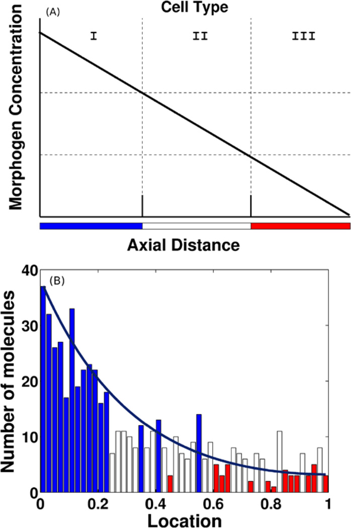
The French flag model serves as a paradigm of PI models (cf. Fig. 1) and captures some essential aspects of pattern formation. The question is how to divide an initially uniform one-dimensional domain into three equally sized sub-domains, and in a PI model this is done by setting thresholds in the morphogen to define the boundary of different types. The deterministic version of how a French flag or three cell types can be produced in 1D, using suitable thresholds in a linear morphogen distribution, is shown in Fig. 1(A).
Fig. 1.
(A) A deterministic version of the French flag problem. (B) One realization of the French flag model based on stochastic dynamics. The bars are color-coded according to the number of molecules in a cell: blue—greater than 12 and white—greater than 6 molecules. (From Kang et al. 2012, with permission)
Most studies of pattern formation have used a deterministic model, but stochastic effects may be important in gene expression and spatial pattern formation if the copy number of some important components is low. For example, in dorsal-ventral patterning of Drosophila, a primary signaling molecule called Dpp is present at concentrations of 10−10 M to 10−9 M (Shimmi and O’Connor 2003), and at these concentrations there are on average fewer than 10 signaling molecules per nucleus in the embryo. To illustrate the effect this may have on patterning, consider the French flag problem. In Fig. 1(B) we show one realization of a stochastic model in which the input flux of morphogen is fixed at the left, and it diffuses into the domain and is degraded by a first order reaction. The solid line shows the steady-state mean of the distribution, which can be computed directly since the equations are linear (Gadgil et al. 2005), and this also represents the steady-state distribution for the corresponding deterministic system. Since each embryo is a single realization of the patterning process, the results illustrate the uncertainty in fixing the location of the boundaries between cell types. Of course the downstream interpretation of the signal, as well as feedback from downstream steps may play a role in reducing the effect of signaling noise, and some examples of this are given in Kang et al. (2012).
In the following section we discuss several different transport processes that occur on different time and space scales which can lead to a diffusion-based description of transport. In later sections we describe several methods for estimating an appropriate cell or compartment size for simulations of stochastic RD equations, we discuss a new computational algorithm for solving discretized RD equations, and in the last section we illustrate some of the issues involved in applying the theoretical analysis to an RD example.
2 Routes to the Diffusion Process
2.1 Classical Diffusion
The motion of point particles under deterministic or random forcing is described by Newton’s law, which we write in the form
| (1) |
| (2) |
Here (xi, vi) ε ℝn, n = 1, 2, 3 are the positions and velocities of the ith particle and mi is the mass. If the imposed forces X and V are smooth deterministic forces they can be written as dXi = Xi dt, and similarly for dV, and (1) and (2) are the standard Newton equations for particles. When Xi and Vi are random forces these are stochastic differential equations, the integral forms of which are interpreted in the Ito sense (Arnold 1974; Capasso and Bakstein 2005). The random forcing terms that are most widely used are Gaussian white noise and compound Poisson processes, both of which are stable Lévy processes (Sato 1999; Applebaum 2004), i.e., stochastic-continuous processes having independent, stationary increments and sample paths that are right-continuous and have left limits.
A general description of Brownian motion of a heavy particle in a fluid is based on (1) and (2), with the assumption that the forcing on position is zero, the random forcing on velocity is Gaussian white noise W, and velocity-dependent frictional forces are admitted. This leads to
| (3) |
| (4) |
where ζ is the friction coefficient, kB is Boltzmann’s constant, and T is the temperature. Under the assumption that the fluid motion relaxes on a much shorter time scale than the motion of the particle, the hydrodynamic forces appear both via the deterministic friction force and the random forces. Under these assumptions (3) and (4) are equivalent to a partial differential equation for the conditional probability density p(x, v, t|x′, v′, t′) of finding the particle at (x, v) in phase space at time t, having started at (x′, v′) at time t′, namely,
| (5) |
This is known as the Fokker–Planck–Kramers–Klein equation (Wilemski 1976), or simply the Fokker–Planck equation. The evolution of p is driven by both drift-diffusion in v and drift in x due to the external force, but when the friction coefficient ζ is large, the velocity relaxes on a time scale 𝒪(ζ−1), and then (5) reduces to the Smoluchowski equation
| (6) |
for the number density n(x, t) = ∫ p dv, where the diffusion coefficient is defined by the relation
The latter equality is the Stokes–Einstein relation for a spherical particle of radius r in a fluid of viscosity η. In the absence of an external force the drift term vanishes and the standard diffusion equation results.
However, this approach only applies when the concentration of the diffusing particle is sufficiently low that inter-particle interactions can be neglected. A more general formulation begins with the ansatz that, other processes and external fields being absent, a spatially non-uniform particle distribution evolves so as to minimize the Gibbs or Helmholtz free energy, depending on the constraints on the system (Callen 1960). Thus a more general description of molecular diffusion leads to the equation
| (7) |
where μ is the chemical potential of the mobile species and M its mobility. This is a more realistic description of diffusion in the complex cytoplasm of a cell, since in general the free energy and hence μ incorporates like–like interactions and like–unlike interactions (Prigogine and DeFay 1954; Othmer 1976).
2.2 Standard and Anomalous Diffusion as the Limit of Space-Jump Processes
An alternate route, which is not predicated on the molecular origin of diffusion, begins with a jump process, either on a lattice or of a more general kind. Now the forces are impulses given, for example, by a Poisson forcing function acting on the position. Thus the particle or walker moves by a sequence of jumps, distributed in time according to a Poisson law, and the position is given by
| (8) |
The amplitudes Yk are independent random variables, H is the step function, and N(t) is a homogeneous Poisson counting process with parameter λ that counts the number of jumps in [0, t], assuming that N (0) = 0 with certainty. A generalization of this allows coupling between the amplitudes of the impulses and their temporal occurrence, and can be defined by a random measure M (dt, dY) that gives the number of jumps in ((t, t + dt) × (y, y + dy)).
More general waiting time distributions for the jumps can be treated as well. Let 𝒯 be the waiting time between jumps, assume they are independent and identically distributed, and let φ (t) be the probability density function (PDF) for the waiting time distribution (WTD). If a jump has occurred at t = 0 then
In general the jumps in space may depend on the waiting time, and conversely, the WTD may depend on the size of the preceding jump, but to make the analysis tractable, we assume that the spatial redistribution that occurs at jumps is independent of the WTD. Let T (x, y) be the PDF for a jump from y to x, i.e., given that a jump occurs at Ti,
| (9) |
where the superscripts ± denote limits from the right and left, respectively. If the underlying medium is spatially non-homogeneous and anisotropic, the transition probability depends on x and y separately, while in a homogeneous medium T (x, y) = T̃ (x − y), where T̃ is the unconditional probability of a jump of length |x − y|. We further assume that T is sufficiently smooth and that for any fixed y the first two x-moments of T are finite—the effect of infinite moments will be discussed later.
Let p(x, t|0) dx be the probability that a walker who begins at the origin at t = 0 is in the interval (x, x + dx) at time t, and let Φ̂(t) be the probability of no jump up to time t. Then p(x, t|0) satisfies the renewal equation
| (10) |
and many of the standard jump processes can be derived from this by particular choices of φ and T (Othmer et al. 1988). For instance, if the WTD is exponential, one obtains the continuous time random walk
| (11) |
which has been widely studied (cf. Weiss 1994 and references therein). If we rewrite this as
| (12) |
it has the form of a master equation, which will be discussed later.
It follows from the central limit theorem applied to the sum of the IID steps taken in the walk that any jump process with (i) a WTD that has a finite first moment and (ii) a jump distribution that has a finite second moment evolves like a standard Brownian motion for large t. Thus a standard diffusion process emerges from a wide variety of space jump processes under these two conditions. However, when the large-time limit of the mean-square displacement grows either sub- or super-linearly the process is said to exhibit anomalous diffusion. For example, if
for β ≠ 1 and t → ∞, it is called subdiffusion if β < 1 and superdiffusion if β > 1 (Metzler and Klafter 2000). Subdiffusion occurs when particles spread slowly, whether because they rest or are trapped for a long time, and in particular, if the mean waiting time between jumps is infinite. For example, if the WTD is given by
then the moments Mk are infinite for all k ≥ 1, and one finds from the Laplace transform that
and thus the process is subdiffusive (Othmer and Xue 2013). The superdiffusive case arises when the walk is highly persistent in time. For example, if the walker never changes direction this leads to a wave equation for which the mean square displacement scales as t2.
2.3 Diffusion as the Limit of Poisson-Driven Velocity-Jump Processes
A second class of transport processes that can be described as a diffusion process on certain space and time scales is called the velocity-jump process (Othmer et al. 1988). Again we use position and velocity as the primary variables, but instead of jumps in space we introduce jumps in velocity at random instants. Let p(x, v, y, t) be the density function for individuals in a (2n + m)-dimensional phase space with coordinates (x, v, y), where x ε ℝn is the position, v ε ℝn is the velocity, and y ε ℝm is the set of intracellular state variables involved in cell movement. As in the case of space jumps, we suppose that the waiting time between jumps and the changes in velocity are independent, and that the WTD is exponential. As a result, the turning can be described by the turning rate λ, and the turning kernel T (v, v′), which defines the probability of a change in velocity from v′ to v, given that a reorientation occurs. T (v, v′) is non-negative and normalized so that ∫ T (v, v′) dv = 1, and at present we assume that it is independent of time and space. The evolution of p is then governed by the equation
| (13) |
and the underlying stochastic process is called a velocity jump process. Under suitable assumptions on the turning kernel the parabolic scaling τ = ε2t and ξ = εx, where ε is a small dimensionless parameter (e.g., ε ~ 𝒪(sT/L) with L the domain size, s a characteristic speed, and T a characteristic time), leads to a diffusion approximation of the transport equation. If we neglect the force F and the internal variables, then
| (14) |
where the subscript on ∇, which we drop hereafter, indicates differentiation with respect to the scaled space variable. The right-hand side of (14) is 𝒪(1) compared with the left-hand side, whatever the magnitude of p, and this leads to a diffusion equation for the lowest order term p0 of an outer or Hilbert expansion, which we write as
| (15) |
An approximation result for any order in ε that provides a bound on the difference between the solution of the transport equation and an expansion derived from the solution of the associated parabolic diffusion equation has also been proven (Hillen and Othmer 2000).
Theorem 1 Given suitable assumptions on the turning kernel and the Hilbert expansion (15), p0 solves the parabolic limit equation
| (16) |
with diffusion tensor
| (17) |
In addition, the first two of the higher-order corrections are given by
where ℱ is the pseudoinverse of the turning operator ℒ, V ⊂ ℝn is a compact set and ω = |V|. Then for each ϑ > 0 there exists a constant C > 0 such that for each ϑ/ε2 < t < ∞ and each x ε ℝn, satisfies
The constant C depends on V, D, ϑ and the second eigenvalue μ2 of ℒ.
Therefore, on suitably chosen time and space scales that in essence guarantee that individuals turn frequently enough and thus do not, on average, move too far, the velocity jump process can be approximated by a diffusion process. Such restrictions are easily understood when it is realized that some individualsmay simply continue in their original direction and never turn (Hillen and Othmer 2000).1 This result applies as well when reactions occur and has led to a better understanding of how individual-level behavior leads to the classical Patlak–Keller–Segel chemotaxis equations (Erban and Othmer 2005, 2007), and to macroscopic, individual-based models of bacterial pattern formation (Xue and Othmer 2009; Xue et al. 2011).
The general conclusion is that diffusion processes arise from a variety of more fundamental processes at the molecular or higher level, and in general are an approximation valid only on appropriate time and space scales.
3 The Stochastic Description of Spatially Discrete RD Systems
A master equation is essentially a balance equation that expresses the conservation of probability for a Markovian stochastic process. The form of a master equation depends on whether the state space is discrete or continuous, and whether time is discrete or continuous. An example of a continuous-time, continuous state space process is the space-jump process that led to (12). All such equations can be derived from the fundamental description of a Markovian process given by the Chapman–Kolmogorov equation. In this section we introduce a master equation for reaction–diffusion processes in which the underlying physical space is discretized into Nc compartments of equal volume h3.
Suppose that in each cell there are s distinct species and Nr reactions amongst them. In the stochastic description of reactions and transport the evolution of the system is modeled as a continuous-time Markov jump process. Let N(t) = (N1 (t), N2 (t), …, NNc (t)) be the vector of random variables whose kth vector component represents the number of molecules of species in the kth compartment. Let P(n, t) be the probability that N(t) = n, i.e., the joint probability that. Then P (n, t) ≡ P (n1, n2, …, nk, …, nNc, t). For any reaction network one defines a set of complexes that represent combinations of molecules that react as a unit in a reaction, a map ℰ that encodes the topology of the reaction network, and a map ν that converts complex concentrations into species concentrations. One can show that the ℓth reaction C (k) → C (k′) induces a change Δn(ℓ) = ν ℰ(ℓ) in the number of molecules of all species after one step of the reaction, where subscript ℓ denotes the ℓth column of ℰ and C (k) denotes the kth complex (Gadgil et al. 2005). Therefore the state m = n − ν ℰ(ℓ) is a source or predecessor to n under one step of the ℓth reaction. Similarly, states of the form m = n + ν ν(ℓ) are reachable from n in one step of the ℓth reaction. Once the graph of the network and the stoichiometry are fixed one can easily derive the explicit form of the master equation for a given network of reactions from the corresponding deterministic equations (Gadgil et al. 2005).
In the presence of diffusive coupling between compartments, the flux of the ith species from k to one of its neighbors k′ is assumed to be given by
| (18) |
while the reverse flux is
The transfer of one molecule in the first step involves the change whereas the reverse flux involves the change . The general form of the master equation for both reaction and diffusion processes is
| (19) |
where 𝒩 (k) is the set of all neighbors of k in the reaction graph for the cellular network and ei = (0, 0, …, 1, …, 0)T has a 1 in the ith position and zeroes elsewhere. The formulation in (18) and (19) is based on the assumption that the domain is decomposed into equal-size compartments. If the compartments have side lengths that are different in different directions then the flux at (18) must be scaled by the h appropriate for each direction, and the sum over neighbors in (19) must be changed to reflect this.
3.1 The Maximal Compartment Size
Given the reaction network and the network of connections between cells, one must next determine the appropriate cell size. The question as to how large it can be has been addressed by many, and a variety of criteria have been proposed (Kang et al. 2012). Most are based on first estimating the smallest reaction time scale and then choosing a compartment size to ensure that the diffusion time scale is less than this. Since the diffusion time in a cube of side h scales as h2 / D, one has to compare the kinetic rate for the fastest step with the slowest diffusion rate. Alternatively one could generalize this by treating each reaction separately and first applying the criterion to the species involved in a given reaction, and then comparing the estimates for all reactions. Later we will discuss a result that determines a suitable time scale for the entire network and use this to set the cell size.
Typically the accuracy of a numerical solution of deterministic continuum RD equations increases as the grid size is reduced, but this not true for RD master equations such as (19) without further analysis. To see this, consider a closed system of fixed size that contains N molecules, and suppose that the system is discretized into Nc compartments that are connected by diffusion. The stationary distribution is spatially uniform and multinomial (Gadgil et al. 2005), with mean and variance given by
An appropriate measure of the fluctuations is the coefficient of variation, CV = σi / Mi, and this is
| (20) |
which is zero for Nc = 1 and which grows as for large Nc. Thus this measure of the fluctuations tends to infinity as Nc → ∞. However, as is shown in Kang et al. (2012), a suitably scaled CV defined later stabilizes as Nc → ∞ and the evolution equation for the corresponding scaled mean value converges to the continuum RD equations for linear reactions. Later the onset of the plateau in this scaled CV as a function of Nc is used to set the compartment size. If bimolecular reactions are involved there are also lower bounds on the size because each compartment must be large enough to contain both reacting species, and the continuum limit of the RD master equation does not capture such reactions (Isaacson 2009). To circumvent this one has to allow reactions between molecules in adjacent compartments (Agbanusi and Isaacson 2013).
An alternate criterion for determining the maximal compartment size is based on the deterministic RD equations for a reaction network. The basic premise is that the cell size must be small enough so that if one were to impose no-flux boundary conditions on the cell boundary, the solution would relax to a spatially uniform solution, whether stationary or periodic. This requires that diffusion dominates reaction in an appropriate sense, and that was first made precise in Othmer (1977), Ashkenazi and Othmer (1978) and generalized in Conway et al. (1978). Let c be the vector of species concentrations let c̄ be the spatial average of c, and let δ be the smallest diffusion coefficient and α1 the largest non-zero eigenvalue of the Laplacian with homogeneous Neumann conditions on ∂Ω. Then it was shown that under the assumption that all species diffuse, ∥ c (x, t) − c̄ (t) ∥L2 → 0 exponentially in t in any bounded domain Ω ε ℝn if |α1 δ | > r̂, where r̂ is the maximum Euclidean norm, taken over an appropriate invariant set C∞, of the Jacobian of the reaction terms. This result was extended in Kang et al. (2012) to allow non-diffusing species and reactions at the boundary, as described below. We briefly describe this result here and later use it to compute a maximal compartment size for a discretized reaction–diffusion system. We discuss conditions for the existence of an invariant set there.
Let Ω ⊂ ℝ3 be a domain with a smooth boundary ∂Ω, and let u (x, t) ε ℝm and υ (x, t) ε ℝn denote the concentrations of diffusing and non-diffusing species, respectively, that react in Ω at time t. We redefine the vector c = [uT, υT]T of species concentrations and assume that c is contained in a closed, invariant rectangle C∞ at all times. Then, we write the governing equations and the boundary conditions for the species as follows:
| (21) |
We assume that ℛ and 𝒮 are C1 in the non-negative cone of (u, υ)-space, and in general both are nonlinear functions of (u, υ).
The Jacobians of a function f : ℝm × ℝn → ℝm × ℝn with respect to u and υ are denoted
We assume that for all c ε C∞, σ (Dυ 𝒮(c)) ⊂ LHP, where σ (A) denotes the spectrum of A. Then there exists a Lyapunov matrix Wc for which Wc Dυ 𝒮 (c) is uniformly negative. Letting λm (Wc) and λM (Wc) be the smallest and the largest eigenvalues of Wc, we define
| (22) |
Here ∥ · ∥E denotes the Euclidean norm, and U = (u, υ, ῡ), where ῡ is a solution of
and ū is the spatial average of u. The Lyapunov matrix is needed because some species do not diffuse—details are given in Kang et al. (2012). We define measures of kinetic sensitivity via the Jacobians of the reaction terms as
| (23) |
where | · | denotes the absolute value.
Conditions for exponential convergence in time of c (x, t) to a spatially uniform solution under homogeneous Neumann boundary conditions are derived in Kang et al. (2012). In essence these require that the smallest non-zero diffusion coefficient should be large enough compared to some function of the kinetic sensitivities, r̂u,r̂υ, ŝu, and s̆υ, and of the constants, λm, λM, and w, defined by the positive operator Wc. There it was shown that ∥ c(x, t) − c̄(t) ∥L2 → 0 exponentially in t if
| (24) |
where δ = mini 𝒟i and α1 is the largest non-zero eigenvalue of the scalar problem
| (25) |
If all species diffuse this reduces to the previous condition |α1 δ | > r̂u. A kinetic scheme that satisfies the conditions for a Turing instability shows that the conditions can be violated on a general domain, but they can be met on a sufficiently small domain, even for such mechanisms. This criterion will be used later to estimate an appropriate cell size in an example.
3.2 A Generalized Measure of Fluctuations
To assess the fluctuations in the network one can use one of several forms of a coefficient of variation. The first measure results from defining the noise component-and compartment-wise, which may be appropriate when assessing the effect of fluctuations in a morphogen used to define the boundary between two tissue types. In this case one computes the standard deviation of the number of molecules for the ith species in the kth compartment divided by its mean, viz.,
| (26) |
where η = (k, i). This reflects the fluctuations of each species in each compartment, and thereby leads to a total of sNc measures. However, for most purposes a single global measure that averages over all species and compartments is more appropriate. Among the many ways to do this, we later use a measure based on a normalized covariance matrix, which is defined as (Tomioka et al. 2004)
where ζ= (q, j) and the index function i labels the component. We then define a generalized coefficient of variation as the square root of the maximum eigenvalue of Σ0(t), and denote it
| (27) |
Since the covariance matrix is symmetric and at least positive semi-definite, this is well-defined. The long-time behavior of this is defined by Σ0,∞ ≡ limt → ∞ Σ0 (t), and the steady-state CV* is given by
In certain classes of linear reaction networks one can prove that CV* is an increasing function of the number of cells, as in the pure diffusion case. In particular, if there are no catalyzed inputs to an open system, or if in a closed system the kinetic matrix has exactly one zero eigenvalue, then CV* is the square root of the reciprocal of the smallest mean molecule number in all cells and tends to infinity as Nc → ∞ (Kang et al. 2012). However, it can be shown that a scaled CV* defined as
| (28) |
where V is the total volume of the system, stabilizes as the cell number increases under appropriate conditions (Kang et al. 2012). Moreover, it was shown there that the estimate of cell size derived from the PDE criterion agrees quite well with the cell size at which the scaled CV stabilizes.
In nonlinear problems an analytic expression for the scaled CV has not been established, but whether or not it stabilizes as the cell size decreases can always be checked computationally, and we show in a later section that it provides a reasonable estimate for a nonlinear system.
4 An Exact Algorithm for Simulating Stochastic RD Systems
4.1 A Brief Description of the Original and an Optimized Direct Method
Numerous stochastic simulation algorithms (SSAs) have been proposed since the original exact algorithms, called the first reaction method and the direct method, were formulated by Gillespie (1977). Later Gibson and Bruck (2000) designed the next reaction method in which random numbers generated for the direct method are re-used, and a priority tree is used to accelerate the search for the next reaction. In this section we develop a new algorithm for RD systems, and to set it in context we first describe the original direct method. A comparison with SSAs for RD equations will be done after developing the new algorithm.
We first suppose that the system volume V is well-mixed and that there are Nr reactions amongst s species. The reaction rates can be written
| (29) |
where cℓ is the probability per unit time that the molecular species in the j th complex reacts, j (ℓ) denotes the reactant complex for the ℓth reaction, and hj (ℓ) (n) is the number of independent combinations of the molecular components in this complex, viz.,
| (30) |
Here kℓ is the rate constant for the deterministic rate equations, written in terms of the number density, and νij (ℓ) is the stoichiometric coefficient of species i in the j (ℓ)th reaction.
In Gillespie’s notation, the probability density for reaction type μ is
| (31) |
where
In the Monte Carlo simulation algorithm of the direct method, a basic reaction cycle comprises three steps: first, determine the waiting time for the next reaction; second, determine which reaction will occur; and lastly, update the system state to reflect changes in the species involved as reactants or products in the reaction that has occurred. Accordingly, during each cycle two random numbers R1, R2 ε URN[0, 1] are generated, one of which is used to calculate the waiting time according to
| (32) |
and the other of which is used to determine the next reaction type μ according to
| (33) |
Cao et al. proposed several potential ways of optimizing the original direct method algorithm by reducing the cost of specific steps (Cao et al. 2004), such as preordering the reactions according to their firing frequency and recomputing only the propensities of reactions which are affected by the current reaction.
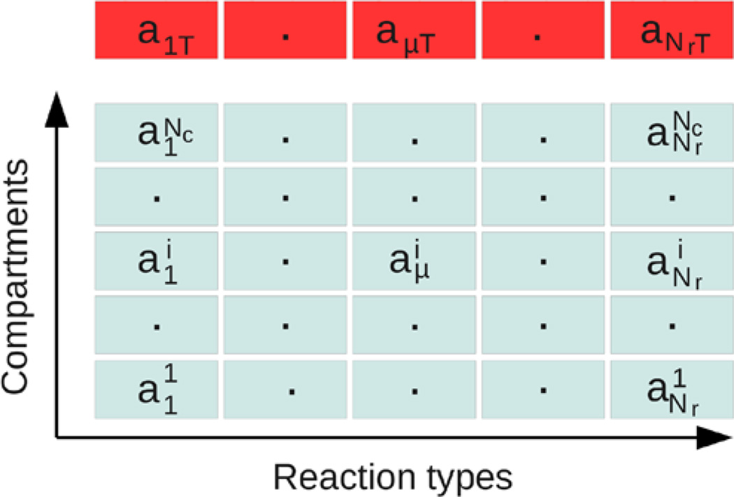
If we apply the direct method to a discretized volume of Nc equal-sized cells, as described by the RD master equation (19), there are a total of Rx = Nr · Nc reactions, which can be large for 3D problems, but an enhanced direct method used for polymer dynamics (Matzavinos and Othmer 2007) can be used here. In this algorithm, reactions of the same type in different cells are lumped into an equivalence class, and the propensity of an equivalence class is simply the sum of the propensities of all individual reactions that belong to that class. For example, if the ‘reaction’ is a diffusion step, then diffusive jumps in all directions among all cells are considered as one class for that species. To determine the next reaction, one first searches for the next reaction type among all equivalence classes, and then, given the reaction type, searches for the cell in which the reaction occurs. The comparison between this algorithm and the direct method is illustrated in Fig. 2, where
| (34) |
and where the superscript i denotes the computational cell. In the original Gillespie method one searches for the next reaction among Nr × Nc cells, while in the optimized algorithm one searches for the reaction type μ among Nr equivalence classes, and then in the column labeled μ searches for the target cell i. The average number of search steps are estimated as 𝒪 (Nr × Nc) and 𝒪 (Nr + Nc), respectively.2 The ratio of search times implies that the improved algorithm leads to a lower search time whenever Nc > Nr / (Nr − 1), and if for example, there are 10 reactions in 1000 cells, the speedup is approximately ten-fold. However, one can do better, as is shown in the next section.
Fig. 2.
Original (bottom) and optimized (top) Gillespie’s direct method applied to reaction diffusion systems
4.2 A New Search Algorithm for Discretized RD Equations
Earlier we showed how to predict a maximal compartment size, and later we will show in an example that this size may be so small that Nc may easily be of the order of thousands or tens of thousands in a 3D system. When Nc is large, the search time for the target cell as described above will dominate the total computational cost, and could present a significant bottleneck for simulations.
Therefore we developed an optimized search algorithm that is based on a subdivision of the computational cells into blocks, and which incorporates the previously defined equivalence classes. Associated with each block is the sum of propensities for each reaction type within individual cells contained in that block, and, instead of searching for target cells sequentially among the Nc cells, one first determines which block the target cell belongs to, and then searches for the cell within that block. Suppose we group all cells into m disjoint blocks, of which each includes Nc/m cells.3 One needs 𝒪 (m) steps to find the target block, and within that block, one needs another 𝒪 (Nc / m) steps to determine the target cell. Accordingly, one needs only 𝒪 (m+ Nc/m) search steps instead of 𝒪 (Nc).
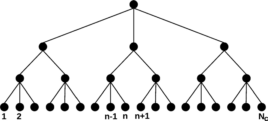
One can generalize the above procedure by defining a tree structure as shown in Fig. 3. The root is a node that reflects the propensities of all reaction types, which in turn are the sum of propensities of corresponding reaction types in all daughter nodes linked to the root, and similarly for each level in the tree. In the lowest level the nodes are simply the computational cells, and based on this construction, the total propensity of a reaction type is simply the sum of the propensities of that reaction among all the computational cells. Searching for the target cell in the tree is a straightforward top down search, as in a decision tree.
Fig. 3.
The tree structure used in searching for the current reacting cell. In this tree, there are a total of (NL +2) levels, where the root is the 0th level, and the nodes at the lowest (i.e., (NL +1)th) layer are the computational cells. We assume each node in the ith level (i ε {0, 1, …, NL}) has mi+1 daughters
We call the resulting algorithm for a tree with (NL + 2)-levels an NL-partition algorithm—the detailed steps are given later. The root is designated as the 0th level, and the lowest level, which contains all computational cells, as the (NL + 1)th level. For the sake of simplicity, we assume an equal number of daughter nodes for any node in the same level. Let each node in the ith level have mi+1 daughter nodes; then . In such a tree, searching for the target cell through NL + 1 levels takes
| (35) |
steps whereas updating the tree structure after the current reaction takes
| (36) |
steps, where gj denotes the number of reaction propensities at the jth cell affected by the current reaction step. Note that if the current step is a diffusive jump, there will be more than one non-zero g-term, whereas when the current reaction is a non-diffusion reaction, there will be only one non-zero g-term. The value of each g-term indicates the complexity of the inter-connection between reactions, and thus (36) encodes both information on diffusion and reactions in the system.
4.3 The Algorithm in Detail
To explain the algorithm in detail, we define the following additional quantities.
: number of reactant combinations of reaction type μ in the ith cell, i = 1, …, Nc.
: reaction rate of reaction type μ in the ith cell, i = 1, …, Nc.
hμT: total number of reactant combinations of type μ among all cells: .
aμT: total rate of reaction type μ among all cells: .
a0: total reaction rate of all types in all cells: .
- Initialization steps
- Partition the system domain into Nc computational cells. Each cell is associated with a data structure with information local to the cell, such as the numbers of each molecular species, the rate constants of reactions (cμ), the reactant combinations (), etc.
- Create a tree structure with nodes as in Fig. 3. Assign the propensity vector of all reaction types to each node, using the fact that for the interior levels the propensity of a reaction type at a node is the sum of the propensities of that type in all daughter nodes attached to the node.
- Initialize the computational cells and reaction rate tree corresponding to the initial condition of the system.
-
The time stepping procedure
Suppose that the simulation time is tn after n reaction steps. Let the state of the system evolve as follows.- Generate a random number R1, and compute the waiting time τn as
where and aμT is stored in the propensity vector associated with the root node of the tree. -
Generate a second random number (R2) to determine the type and cell location of the next reaction.
- The reaction type μ is such that 1 ≤ μ ≤ Nr and
-
To determine the target cell, first compute the random number Q ε URN[0, a0] given byThe target cell d in which the next reaction occurs is found by searching top down through the reaction tree until
(37)
In detail, first examine the m1 nodes at the first layer of the propensity tree structure in Fig. 3, and find the smallest m1μ such that m1μ ≤ m1
where is the propensity of reaction type μ associated with the ith node at the first layer. After that, replace Q by(38)
and examine the m2 nodes connected with the m1μst node at the first layer, and find the smallest m2μ such that m2μ ≤ m2 and(39) (40) Repeat the above procedure until the lowest layer is reached and the target cell is found. A path from the root to the target cell will be represented by the vector (m1μ, m2μ, …, m(NL+1)μ), which means that the path passes through the m1μ th node connected with the root, and m(i+1)μ signifies that the path passes through the m(i+1)μ th node connected with the previous node of the path. - Update the state of the affected cells based on result (b). First, one changes the molecular numbers and reactant combinations of the affected reactions in those cells. To update the tree, suppose that at the ith cell reaction type j changes its reactant combinations from to Let ; then for any branch points on the path from the computation cell to the tree root, add to the reactant combination at that point.
Advance the time from tn to tn+1 = tn + τn, and repeat step (2) until the desired time is reached.
4.4 Estimates of the Cost of Searching and Updating in Three Algorithms
In the following we will focus on three specific partition algorithms depending on the number of levels in the tree. First is a one-level partition algorithm (G1) obtained by dividing Nc cells into m1 groups. In reference to the tree in Fig. 3, the second level contains m1 nodes, each of which links to Nc/m1 cells. The second algorithm is a two-level partition algorithm (G2) obtained by making a tree structure with a root connecting to m1 daughter nodes, each of which in turn connects to m2 nodes. The latter nodes each connect to Nc/(m1 · m2) computational cells. The third algorithm is the extreme case of a binary tree (Gbinary) in which each node in the tree has two daughter nodes. Later the efficiency of these algorithm is compared when they are applied to two simple examples.
When Nc is large, searching for the target reacting cell through the tree structure and subsequent updating could be costly. In searching for the target cell, one goes through the sequential comparison as shown in the detailed procedure in (38) and (40). The number of comparisons made in finding the target cell, which involve both vertical steps and horizontal comparisons, is called the search depth. In updating the tree after a reaction occurs, the changed propensity in an affected cell must propagate from that cell to the root node, and therefore (NL + 1) updating steps are needed. The average searching and updating steps in a reaction cycle for a uniformally distributed system are summarized in Table 1 for different algorithms. The optimal parameter for each algorithm is predicted under the present assumption that Nc is large.
Table 1.
Comparison of searching and updating steps in three algorithms
| Algorithm | Nsearch | Nupdate | Optimal parameter | Optimal Nsearch | ||||
|---|---|---|---|---|---|---|---|---|
| G1 | ||||||||
| G2 | ||||||||
| Gbinary | log2(Nc) | log2(Nc) |
4.5 A Numerical Comparison of Three Algorithms
Next we apply the three algorithms described in last section to two examples.
4.5.1 Pure Diffusion of One Species
The first example is a comparison of the efficiency of the three algorithms when simulating pure diffusion of one species on a quasi-2D domain. We use a domain of size 6.4 µm × 6.4 µm divided into 64 × 64 rectangular compartments of size 0.1 µm × 0.1 µm, each of height 0.1 µm. The 5.0 µM concentration, which is equivalent to 12329 molecules or approximately 3 molecules per cell, is uniformly distributed in the domain, and the diffusion coefficient is 2.0 µm2/s. The run time of the test of the algorithms is based on 50 seconds of dynamics.
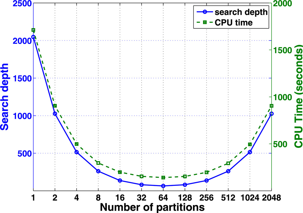
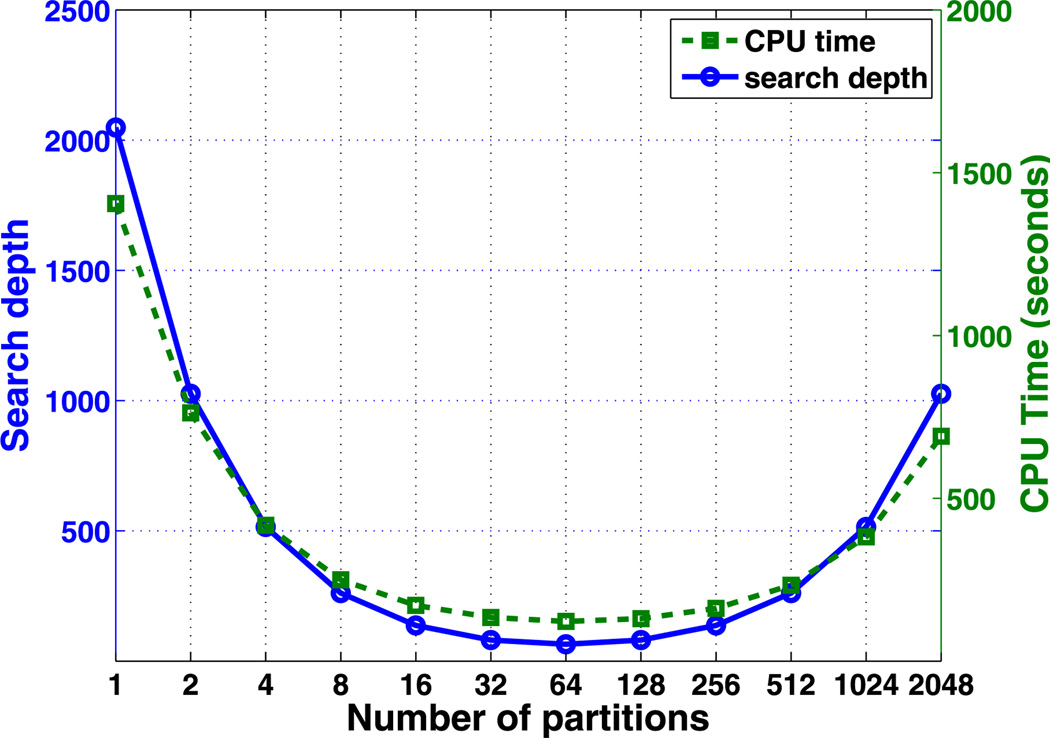
First, we test the CPU cost using algorithm G1. The search depth and total CPU cost for different cell segmentation is summarized in Fig. 4. The numerical simulations show that the total CPU cost is dependent on how the computational cells are partitioned into groups (i.e., m1). Both the search depth and the CPU cost are convex functions of the partition number. The minimum search depth Nsearch and the CPU cost occur at the same optimal partition, which is predicted to occur when the partition number . In the current simulation, Nc = (Lx/Δhx) · (Ly/Δhy) = 4096, which gives the optimal m1 = 64. The optimal algorithm with m1 = 64 is more than ten-fold faster than that without partitioning i.e., when m1 = 1.
Fig. 4.
The search depth and CPU cost of algorithm G1 in pure diffusion of one species
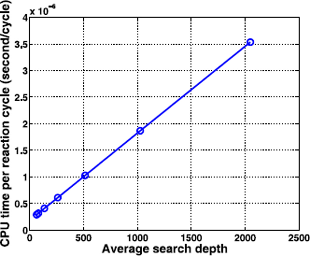
According to step (2) in the detailed algorithm, the CPU time for each reaction type consists of the cost for the following operations: generation of two random numbers, determination of the target reaction type, searching for the target reacting cell, and updating the tree and the system configuration. For G1 algorithms with various cell partitions, the costs are constant for the above operations except for the cost of searching for the target cell. Thus, it is reasonable to postulate that the CPU cost (CCPU) in a typical reaction cycle is linearly related to the average search depth (ASD), i.e.,
| (41) |
where C0 is the total machine cost for all operations except for the searching step, and C1 is the CPU time cost for each search step. Note that in the detailed algorithm, a typical search path for the target cell, say (m1μ, m2μ, …, m(NL+1)μ), will have a search depth of . The numerical results confirm the linear dependence of the average CPU cost on the average search depth, as shown in Fig. 5. In particular, for pure diffusion of one species, the numerical computation in Fig. 5 shows that (C0, C1) = (1.84 × 10⁻⁷, 1.64 × 10⁻⁹) given the data structures in the current implementation. Therefore, the sum of the updating and other costs is equivalent to 1.84 × 10⁻⁷ / 1.64 × 10⁻⁹ ≈ 112 searching steps. One thus predicts that the original Gillespie direct algorithm without optimization of the searching step can be accelerated by -fold using the G1 algorithm, which is approximately 12 with Nc = 4096 in the current example.
Fig. 5.
The linear dependence of CPU time per reaction cycle on the average search depth in algorithm G1. The search depth of the circled points corresponds to cell partitions m1 = 64, 32, 16, 8, 4, 2, 1
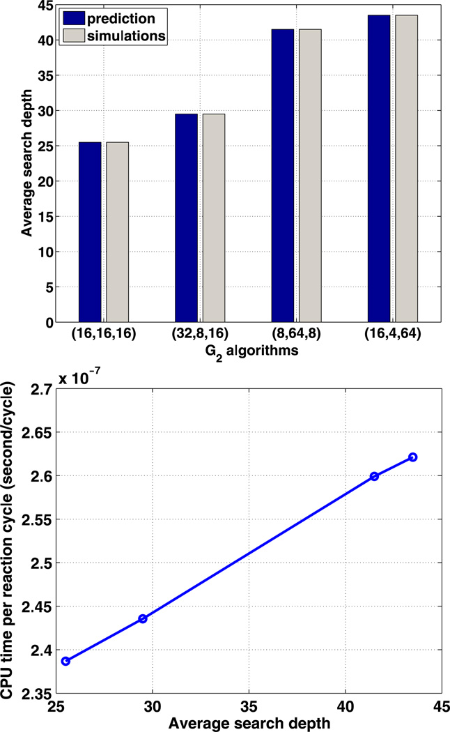
We also ran the simulation using algorithm G2. As previously described for the tree structure in Fig. 3, this algorithm requires three parameters, m1, m2 and m3, but only two are independent since their product is Nc. We fixed the total number of computational cells to be Nc = 4096, and tried different values for (m1, m2, m3). For uniform species distribution, the theoretical prediction of the average search depth for a reaction cycle in Table 1 is confirmed by the stochastic simulations, as shown in Fig. 6 (top). As in algorithm G1, the time for updating the tree structure is negligible compared with the time for the searching steps. The average CPU cost per reaction cycle is also a linear function of the average search depth as in (41), and the function fitted in Fig. 6 (bottom) gives (C0,C1) = (2.06 × 10⁻⁷, 1.33 × 10⁻⁹). Thus the cost of other operations in an average reaction cycle is approximately equal to that of 155 searching steps. The minimal average search depth occurs when , where the CPU cost is least.
Fig. 6.
The average search depth (top) and the dependence of CPU time on search depth (bottom) for four G2 algorithms, each characterized by a choice of three parameters (m1, m2, m3)
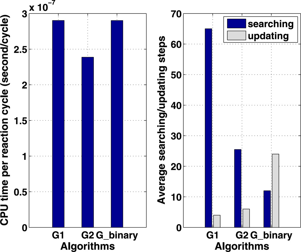
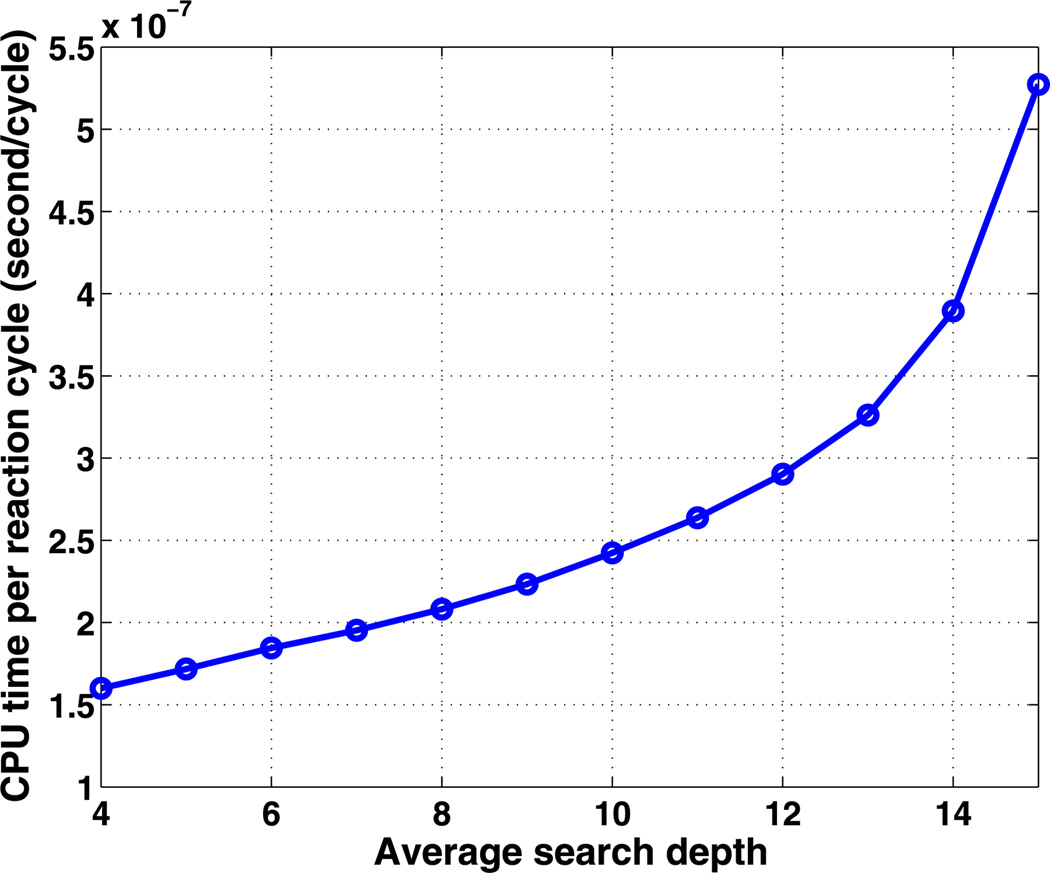
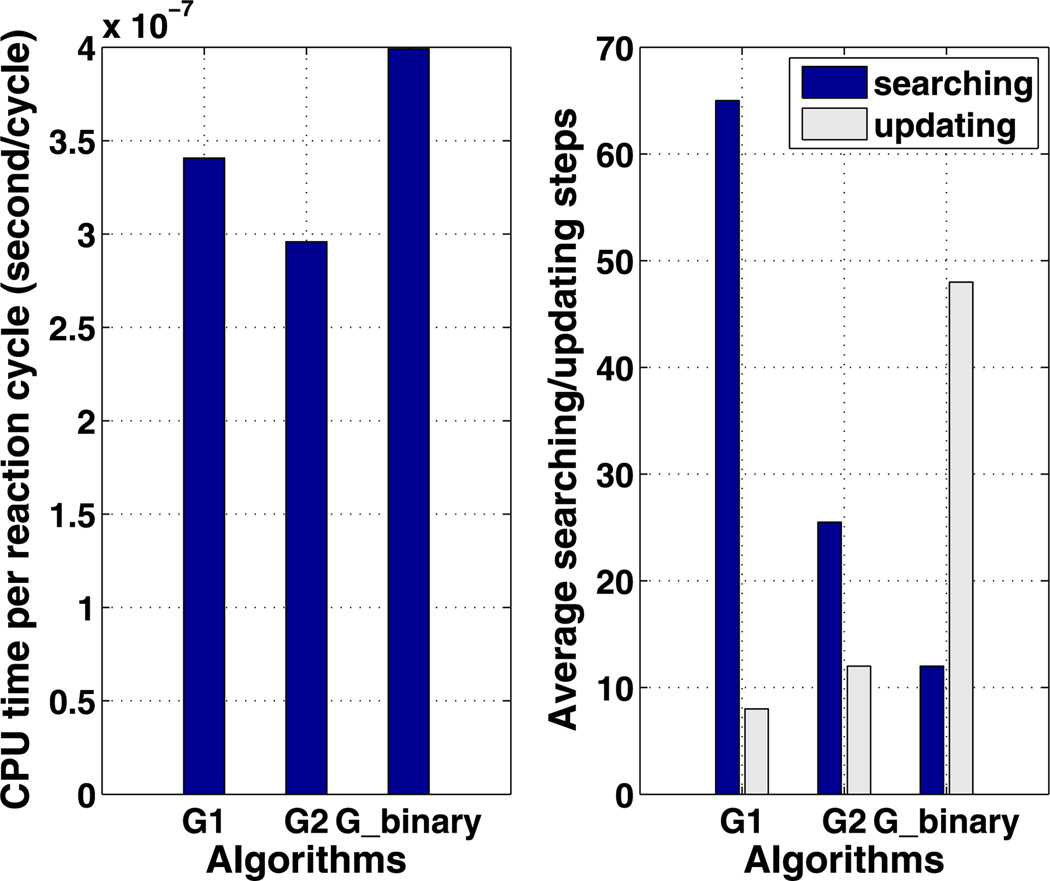
We also tested the efficiency of algorithm Gbinary on this example. For a fixed array of Nc cells, the tree structure associated with this algorithm is unique, unlike the previous two algorithms, which have variable parameters. Therefore, the search depth is log2 (Nc), and the number of updating steps is 2 log2 (Nc) in this example. A comparison between the three algorithms is summarized in Fig. 7. We discover that the optimal G2 algorithm is faster than optimal G1 algorithm by reducing the searching steps efficiently. Although the searching and updating steps are both logarithmic in Nc for Gbinary, this algorithm is not as efficient as G2. To understand this, we plot the CPU cost per reaction cycle as a function of the average search depth for algorithm Gbinary in Fig. 8. One sees there that the CPU cost is a highly nonlinear function of ASD over the range of search depths shown. The authors postulate that the searching/updating of the tree structure between levels is costly, whereas the searching amongst the lateral nodes within each level is cheaper given the data structure we are using in the simulation. Therefore, even though algorithm Gbinary requires less searching and updating steps, algorithm G2 uses more lateral searching rather than vertical searching in the tree and thus outperforms Gbinary. Thus for large Nc, the most efficient algorithm with our optimization strategy is one with a tree structure that optimizes the combined lateral searching and vertical searching, which suggests tree structures with a small number of levels, rather than the binary tree used for Gbinary. When the reaction network is complicated, species become more interconnected, and a reaction firing may affect the propensity of many other reactions, thereby lengthening the updating time in Gbinary.
Fig. 7.
The average CPU cost per reaction cycle (left) and numbers of searching/updating steps (right) are compared among the algorithms of G1, G2 and Gbinary
Fig. 8.
The dependence of the average CPU cost on the average search depth for the Gbinary algorithm
4.5.2 A Three Species Reaction–Diffusion System
In this example, molecules A and B bind reversibly and produce C. Only A and B can diffuse freely on the domain of size 6.4 µm × 6.4 µm × 0.1 µm. The domain is divided into cubes of side length 0.1 µm. The initial concentrations of A, B and C are 5.0, 2.0, and 0.0 µM, respectively. The on- and off-rates of the reaction are 1.0 µM−1 s−1 and 1.0 s−1. The diffusion coefficients for A and B are 2.0 and 1.0 µm2/s, respectively.
As shown in Fig. 9, algorithm G1 is optimal when partitioning the cells into groups, as we predicted in the previous section. The CPU cost is also linear in the average search depth.
Fig. 9.
The search depth and CPU cost of algorithm G1 in a three species RD system
As for the pure diffusion problem, we compare the efficiency of three algorithms in simulating the three species system, and the results are summarized in Fig. 10. As in last example, algorithm G2 is the most efficient among these three. However, with more reactant interactions in the system, the occurrence of one reaction affects more reactions in the next round, with the result that the updating of Gbinary is more costly, and this leads to slower performance of Gbinary than that of G1. As predicted in Table 1, the update cost is proportional to , which is the total affected reactions in all cells after the current reaction step. The current example gives rise to a higher average of total affected reactions due to the more complex reaction network, and the updating steps increase, as seen in a comparison of Fig. 7 and 10.
Fig. 10.
The average CPU cost per reaction cycle (left) and the number of searching/updating steps (right) are compared among the optimal algorithms for G1, G2 and Gbinary
4.6 Other SSAs for RD Equations
There have been numerous applications of the direct method and next reaction method to spatially inhomogeneous systems by compartmentalizing the domain and regarding reactions in different compartment as distinct reactions (Ander et al. 2004; Cao et al. 2004; Li and Petzold 2006). Cao et al. (2004) carefully examined and compared the computational performance of the direct method and next reaction method. They showed that an optimized direct method (ODM) could outperform the next reaction method except for a class of very loosely coupled systems. This is due to the high computational cost in maintaining the inherent data structure in the next reaction method, although the method has less computational operations. Li and Petzold (2006) improved the ODM further by proposing the logarithmic direct method (LDM) with a binary search tree. In the LDM, an array of Nc accumulated partial sums of propensities among all cells is created, on which a binary search is conducted. Even though searching for the target cell could be as fast as logarithmic in Nc, the updating of the array could be expensive. In that algorithm, the array is updated upward from the first partial sum which was changed by the current reaction. Thus, if it is the first of the array of partial sums that changes, the remaining Nc − 1 partial sums must be updated. For large Nc this again may become the bottleneck for this algorithm.
Another algorithm, called the next subvolume method (NSM), was proposed by Elf and Ehrenberg (2004). The next subvolume method (NSM) combines the next reaction method for determining the reacting subvolume in which the next reaction or diffusion occurs, with Gillespie’s direct method for determining which reaction or diffusion step occurs in that subvolume. There is no optimization in the NSM algorithm.
In the algorithm developed here a tree structure defined on the set of computational cells is used to facilitate the searching and updating procedures. There are two major parameters associated with the tree—the number of levels in the tree and the number of daughter nodes emanating from a parent node at each level. One can optimize the performance of this algorithm by testing benchmark problems with varying parameters. As analyzed above, for a fixed tree depth there may be an optimal partition within levels. When the tree depth becomes larger, the search depth decreases whereas the updating steps increase. There may be crossover in the performance of this algorithm when the tree depth increases, due to the increased updating cost. Of course the crossover will depend on the complexity of the reaction network. Our experience suggests that for large problems one should experiment with these numbers to determine the best choices. For instance, one could with tree depths from one to five, and compare the performance with the Gbinary algorithm. But a more rigorous investigation into the optimization problem of the algorithm remains to be done.
Aside from the optimization of partitioning of the compartment, the primary difference between our method and the NSM lies in the order in which operations are performed. We first sum the reaction rates of each reaction type across the subvolumes to decide where reaction occurs (using the direct method) and then search the tree to determine where it occurs. In contrast, the NSM sums all reaction rates in each subvolume, and first determines in which subvolume reaction occurs (using the next reaction method), and then decides the reaction type within the subvolume (using the direct method). Our method is the most highly optimized one using the direct method, and in particular, it eliminates the bottleneck in the LDM method by using a tree structure, which speeds up both the searching and updating steps. However, at present we cannot claim that the algorithm is best for all cases, and a performance comparison between our method and others is needed.
5 Computational Analysis of a Nonlinear RD System
With an efficient computational algorithm for stochastic RD systems at hand, we turn to the analysis of a nonlinear RD system with the objective of illustrating when the deterministic and stochastic descriptions agree and when their predictions differ. While no hard and fast rules can be stated, some cautionary notes on the interpretation of stochastic simulation results emerge. We analyze the deterministic behavior of the system using bifurcation analysis of the PDEs, and compare the predicted dynamics with that from a stochastic description.
Consider the simplified model of the key steps in the glycolytic pathway in a distributed system given in Ashkenazi and Othmer (1978):
| (42) |
with Neumann boundary conditions. The polynomial form of the reaction kinetics is a reduced form of a more complex model of enzyme activations and is used here for ease of analysis (Othmer and Aldridge 1978). In general trimolecular kinetics are not physically realistic.
In order to obtain spatially non-uniform solutions, we assume that 𝒟c1 > 𝒟c2, which is necessary for a Turing instability. To rewrite the equations in a dimensionless form, define the dimensionless variables
| (43) |
where L is a measure of the domain size. The dimensionless equations are
| (44) |
where the Laplacian is now in scaled coordinates. For later comparison with stochastic simulations of this system we will regard the domain as a quasi-1D domain that is rectangular solid of small cross-section in the y and z directions. We focus on the three parameter sets given in Table 2 to illustrate different aspects of the relationship between solutions of the deterministic system (42) and the corresponding stochastic system.
Table 2.
The three sets of parameters used for the dimensionless glycolytic reaction system
| Parameters | Du | θ | δ | κ |
|---|---|---|---|---|
| Set 1 | 2/9 | 0.1 | 2 | 0.1 |
| Set 2 | 2/9 | 0.75 | 0.8 | 0.01 |
| Set 3 | 2/9 | 0.005 | 2 | 0.1 |
5.1 Bifurcation Analysis
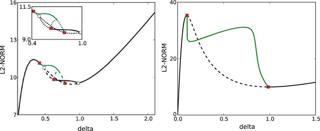
Bifurcation diagrams constructed using AUTO-07P and δ as the bifurcation parameter, with other parameters at the fixed values in Table 2, are shown in Figs. 11 and 12. One sees in Fig. 11 (left) that for an intermediate ratio of the diffusion coefficients there are multiple bifurcations in the range of 0.25–1.0, but at δ = 2, which is used later, there is a unique stable steady state. At a larger ratio of the diffusion coefficients no Turing instabilities are possible and the only bifurcation is to a uniform stable periodic solution that exists for a range of input fluxes (Fig. 11 (right)).
Fig. 11.
The bifurcation diagram with respect to δ, using parameters other than δ as in Set 1 (left) and Set 2 (right) in Table 2. Here and hereafter solid (dashed) lines denote stable (unstable) solutions, open squares denote bifurcation points for static solutions, and filled (red) squares denote Hopf bifurcation points
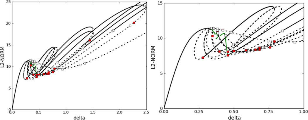
Fig. 12.
The bifurcation diagram (a) and a blowup of one segment (b) with respect to δ using Set 3 in Table 2
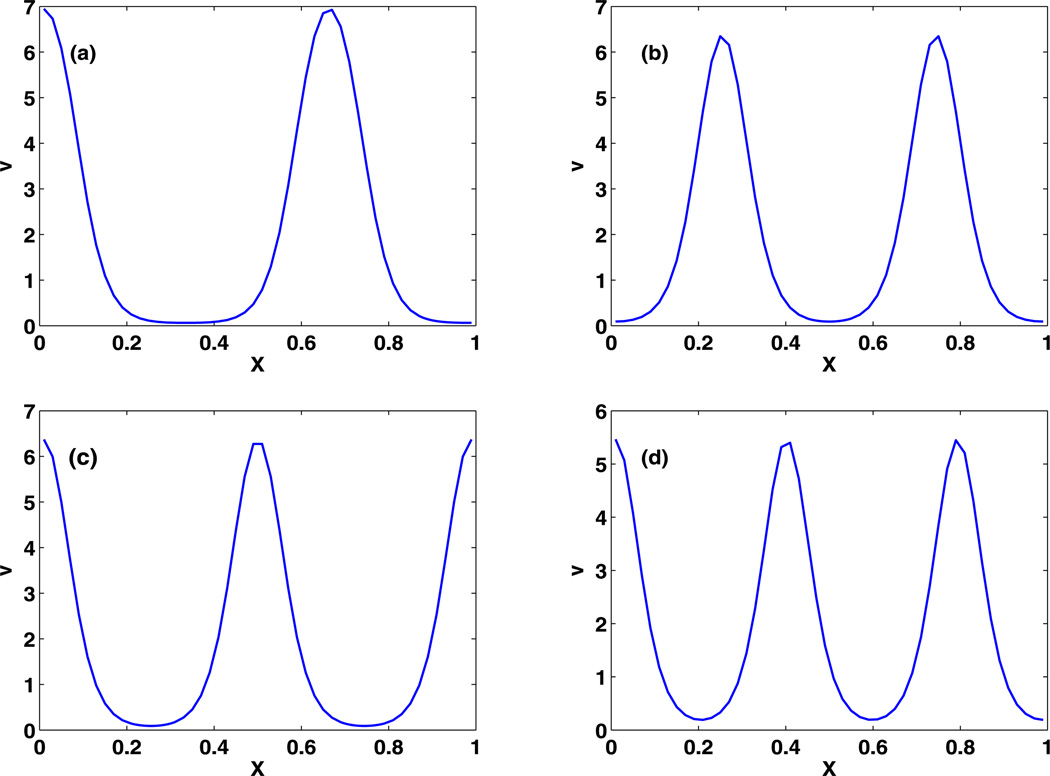
When θ is small enough, as in the third set of parameters, there are many bifurcations and one finds coexistence of multiple stable non-uniform steady states in Fig. 12(a) and in the blowup shown in Fig. 12(b). One also sees that the interaction of the stationary and Hopf branches is very complex, and we have not attempted to resolve all the details. At δ = 2, in Fig. 12, which is the base value in Table 2, there are several unstable and stable steady-state solutions. Some of the stable steady-state solutions are shown in Fig. 13, and there are also symmetry pairs for solutions that are symmetric about the mid-point. In the deterministic simulation, the initial condition uniquely determines the type of the steady-state solution, but later we show that stochastic simulations migrate from one type of solution to another type in time.
Fig. 13.
Coexistence of multiple stable non-uniform steady-state solutions at δ = 2
5.2 An Estimate of the Domain Size
In Sect. 3 we introduced two methods to estimate an upper bound for the maximal compartment size in the stochastic simulation of RD systems. In the first approach using the PDE-driven criterion, one must compute the appropriate reaction sensitivities over a positively invariant region of the local dynamics. With diagonal diffusion, as in the model, that region must be a rectangle (Chueh et al. 1977). However, the polynomial form does not have an invariant rectangle, and therefore we consider the modified system
| (45) |
We have
| (46) |
Therefore, there exists an invariant rectangle, Σ = [0, umax] × [0, υmax], where
| (47) |
Next we derive the maximal cell size, but to simplify the calculations, we do it for the polynomial system. We will see later that the invariant rectangle gives a very conservative estimate of the size. We have
and therefore
We compute where * is the conjugate transpose, and we obtain
The eigenvalues of D(u, υ) ℛ (u, υ)* D(u, υ) ℛ (u, υ) satisfy
and therefore
where
Then
For a one-dimensional system of length 1, α1 = −π2, and therefore the convergence condition becomes
| (48) |
This provides a restriction on the scaled diffusion coefficient 𝒟u of the system, and to convert it to a system size we use (43), and set k1 = 1/µM2 s and k3 = 1 s−1. This leads to the following criterion on the allowable size of the system:
| (49) |
The minimum values of the umax and υmax obtained for the three standard parameter sets are shown in the second column in Table 3.
Table 3.
umax and υmax derived from the invariant region and from the numerical simulation using three sets of parameters in Table 2
| Parameters | Invariant region | Numerical solutions |
|---|---|---|
| Set 1 | (20, 2 + 20/ε) | (4, 4) |
| Set 2 | (80, 0.8 + 80/ε) | (8, 8) |
| Set 3 | (20, 2 + 20/ε) | (4, 8) |
These are rough estimates, and one can do better if one restricts attention to a certain class of initial conditions. To obtain estimates in this way, we numerically solve (44) with parameters given in Table 2, considering only initial data for which both species are zero, and obtain the maximal values given in the third column of Table 3. With these refined estimates we obtain the upper bounds on compartment size shown in the third column of Table 4.
Table 4.
An upper bound of the domain size in the system with three sets of parameters as given in Table 2
| Parameters | Invariant region | Numerical solutions | CVs | Other estimates |
|---|---|---|---|---|
| Set 1 | 0.04 µm | 0.2 µm | 0.3 µm | 0.08 µm |
| Set 2 | 0.03 µm | 0.3 µm | 0.6 µm | 0.08 µm |
| Set 3 | 0.008 µm | 0.03 µm | 0.06 µm | 0.009 µm |
The estimates in the fourth column of Table 4 are obtained by determining the value of Nc at which the CV stabilizes, using 1000 realizations of the system to compute the scaled coefficient of variation in time scaled defined as
where CV* (t) is defined in (27). Stabilization of the stationary value of this was used in Kang et al. (2012) as a criterion to determine a lower bound for Nc, but this does not provide a lower bound when the system has a spatially uniform solution at the steady state. Therefore we consider the transient evolution, and because the reaction system in (42) is spatially homogeneous, we assume that all cells but the first are initially empty, and that the first contains 1000 molecules of each species. Under these conditions (t) can capture how fast spatial non-uniformity diffuses across the domain.
We show (t) at three times for different compartment numbers in Figs. 14–16. In Figs. 14 and 15, (t) stabilizes at Nc ~ 10 and Nc ~ 5, respectively, when t = 0.6 s, which leads to the upper bounds
| (50) |
| (51) |
One sees that the compartment size for parameters in Set 1 is smaller than that with Set 2, because the larger θ and smaller κ in Set 2 imply faster spread of species in the domain.
Fig. 14.
(t) at t = 0.2 s, t = 0.6 s, and t = 2.0 s with different numbers of compartments using Set 1 in Table 2 with spatially non-uniform initial values
Fig. 16.
(t) at t = 0.2 s, t = 0.6 s, and t = 2.0 s with different numbers of compartments using Set 3 in Table 2 with spatially non-uniform initial values
Fig. 15.
(t) at t = 0.2 s, t = 0.6 s, and t = 2.0 s with different numbers of compartments using Set 2 in Table 2 with spatially non-uniform initial values
In Fig. 16 the result is less definitive. One might use Nc = 30 as a minimal number but there are still significant variations in the scaled CV, and if we use Nc = 50 we predict an upper bound of
| (52) |
The smaller size compared with the other estimates results from the smaller θ in Set 3. In this example, the compartment sizes estimated by CV stabilization as in the fourth column of the Table 4 are similar to those estimated by the PDE-driven criterion given in the third column of Table 4.
The last column of Table 4 gives an upper bound of the domain size based on the criterion suggested earlier (Bernstein 2005), which requires that the fastest reaction time scale should be slower than the slowest diffusion time scale. In the system (44), the nonlinear reaction has the largest propensity among the reactions based on the parameters in Table 2 and (umax, υmax) given in the third column in Table 3. This criterion requires that
and using 𝒟u = 𝒟c1/(L2k3) and setting 𝒟c1 = 2 µm2/s and k3 = 1 s−1, we obtain the upper bounds given in the last column in Table 4.
Table 4 shows that the invariant region method and Bernstein’s method give comparable estimates of maximal compartment sizes, and both are significantly smaller than estimates based on solving the PDEs for a restricted class of initial data, or computing the CV from stochastic simulations. One reason for the rough estimation using the invariant region method is because the negative nonlinear term is omitted in the estimation in (46), so the interaction between u and υ cannot be captured in the estimates. The numerical solutions of PDEs give finer estimates but they use both umax and υmax of the PDE solution in (49), although it may not be true that umax and υmax occur at the same time point of the PDE solution. In any case, the results suggest that various criteria should be tested when beginning analysis of a new reaction network.
5.3 Comparison of the Deterministic and Stochastic Dynamics
In this section we compare the deterministic and stochastic behavior of the model for the glycolytic reactions. The three parameter sets given in Table 2 are used here, the first of which leads to a unique uniform steady state, the second to a unique uniform periodic solution, and the third to one of several stable steady states.
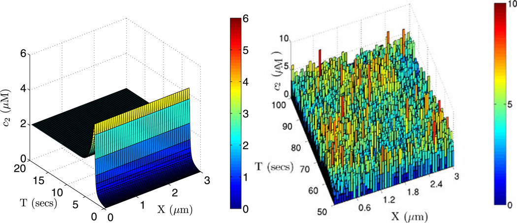
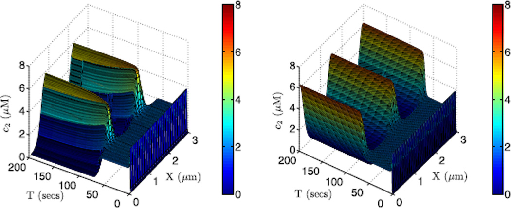
The bifurcation analysis indicates that the RD system corresponding to the first set of parameters has a unique and stable steady-state solution. Starting with uniform zero conditions, the system evolves to the unique stable steady state as shown in Fig. 17 (left). The PDE is solved using 50 grid points in the 1D 3 µm domain on the x-axis. To simulate the dynamics of this 1D system stochastically, we use a rectangular domain of size (3, 0.2, 0.2) µm in the x-, y- and z-directions, respectively. The width in the y- and z-directions is chosen such that it is within the maximal compartment size as estimated previously in the CV analysis. We partition the domain into 50 compartments in the x-direction, and use the optimized search algorithm as described in the previous section to simulate the dynamics. The stochastic simulation indicates that the system approaches a uniform steady state at large times, but due to the small volume of the computational cells, the fluctuation in number of the second species is significant, and the average concentration in individual compartments can be several-fold higher than the steady-state prediction of the PDE. In a typical realization there are about 360 molecules in the entire system.
Fig. 17.
The solutions for the second component of the glycolytic reaction with parameter set 1. The PDE solution with zero initial condition is shown on the left, and on the right is one realization of a stochastic simulation of the system using 50 cells along x-direction of the domain of size (3, 0.2, 0.2) µm
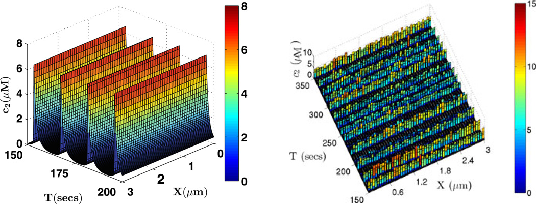
Similarly, we compare the solution of the deterministic PDE and the predictions of the stochastic system (Fig. 18), using parameter set 2 for both. Starting from zero initial conditions, the deterministic system evolves to a periodic solution, which the bifurcation analysis done earlier shows is the only stable solution. The stochastic dynamics also evolve to a periodic solution with similar period (Fig. 18, right), but the fluctuations in the peak concentrations can be large. Despite this, the long-term evolution of the stochastic dynamics reflect those of the PDE prediction with the first two parameter sets, due to the fact that the system has a unique and stable solution in each case.
Fig. 18.
The solutions of the glycolytic RD system with parameter set 2. The periodic solution of the PDE is displayed on the left with 50 grid points on the 1D 3.0 µm domain. On the right is one realization of a stochastic simulation of the system with 50 compartments along the x-axis of the domain of size (3, 0.3, 0.3) µm
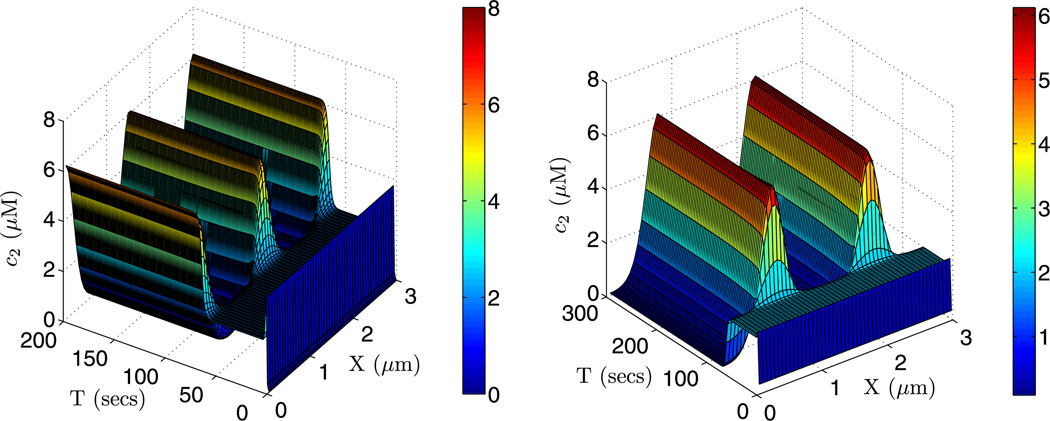
In contrast, the evolution of the RD system using the third parameter set is much more complicated. The bifurcation analysis done earlier based on 50-grid-point discretization of the PDE shows that there are several coexisting uniform and non-uniform steady-state solutions, but only the non-uniform steady states are stable (Fig. 13). As a result, different initial conditions are required to begin in the domain of attraction of different steady states, as shown in Fig. 19. In addition, we find that different discretizations of the PDE may lead to distinct steady states, starting with the same zero initial conditions, as shown in Fig. 20. In all cases the maxima of the solutions are comparable, ranging from 5.5–7.0 µM as was found in the bifurcation analysis.
Fig. 19.
The PDE solution of the glycolytic RD system with parameter set 3. With the same 50-compartment discretization of the 1D 3 µm domain, different initial conditions lie in the domain of attraction of different steady states. In the left panel the initial condition is uniform (c1, c2) = (0, 0) µM, whereas on the right the initial condition is uniform (c1, c2) = (0.1, 0.05) µM
Fig. 20.
Starting with the same zero initial condition, discretizations of the 1D 3 µm domain into 25 (left) and 100 (right) cells lead to different stable steady states
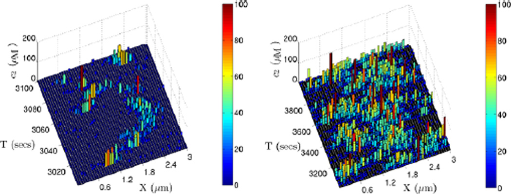
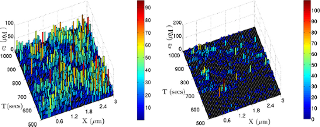
To simulate the stochastic dynamics of this system, we partition the domain into 50 compartments along the x-axis, which yields a maximal compartment size consistent with the CV analysis. We also choose different cross-sectional sizes in the y–z plane but do not further discretize them, and we compare the resulting dynamics. We first use a cross section that lies within the maximal compartment size, which is 0.06 µm. An example of the dynamics in this discretization indicates that the stochastic simulation results are quite different from those of the deterministic prediction of the PDE. As shown in Fig. 21, the evolution of the stochastic simulation shows no clear spatial pattern, and in particular, it is far from the distinct three-peak non-uniform steady state shown in Fig. 19 (left).
Fig. 21.
The evolution of one realization of a stochastic simulation of the glycolytic RD system with parameter set 3. The domain (3, 0.05, 0.05) µm is divided into 50 cells along the x-axis. The dynamics for 100 seconds and 1000 seconds are shown on left and right, respectively
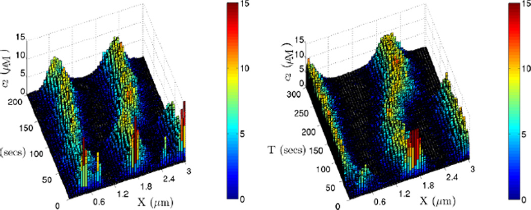
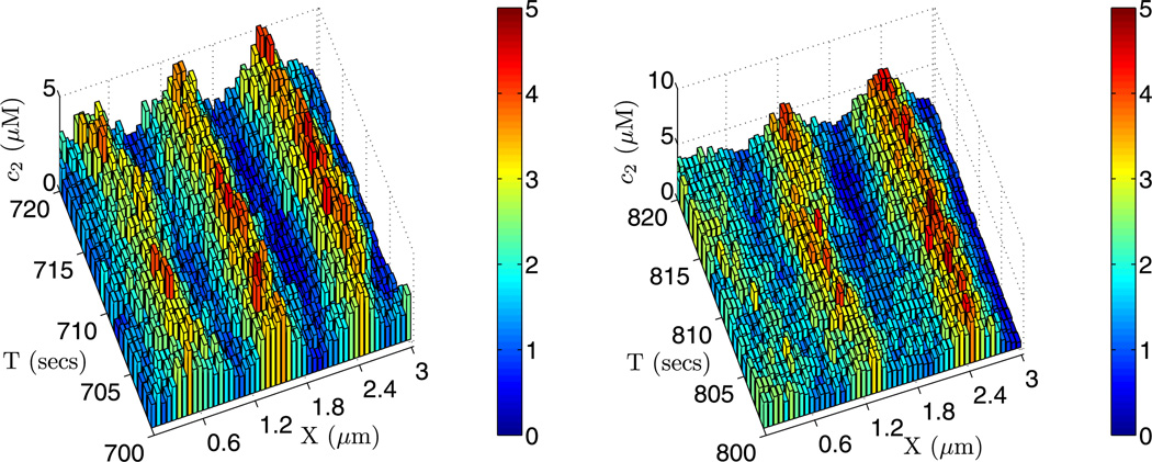
However, if we increase the cross-sectional area of the compartment in the y–z plane to 0.5 × 0.5 µm2, and scale the kinetic coefficients appropriately for the increase in volume, the system evolution shows clearly identifiable pattern formation with spatial distributions corresponding to different steady states predicted by the bifurcation and PDE analysis. Different initial random seeds for the optimized Gillespie algorithm result in completely different behavior of both dynamic and long-term behavior of the system, as indicated in Fig. 22. These simulations show at least two features of the stochastic dynamics of this nonlinear system. Firstly, depending on the initial seed, the intrinsic fluctuations in the stochastic system may lead to stationary distributions that are very different from the stable steady states for the PDE, and secondly, during the early dynamics, the system may migrate from one stable steady state of the PDE to another. However, the results suggest that the final stationary distribution that the system evolves to has a large enough domain of attraction that the fluctuations do not drive the system from this distribution.
Fig. 22.
The evolution of two realizations of the glycolytic RD system with parameter set 3. The domain (3, 0.5, 0.5) µm is divided into 50 cells along the x-axis. Different random number seeds lead to different steady states: that corresponding to Fig. 13(b) on the left and Fig. 13(a) on the right
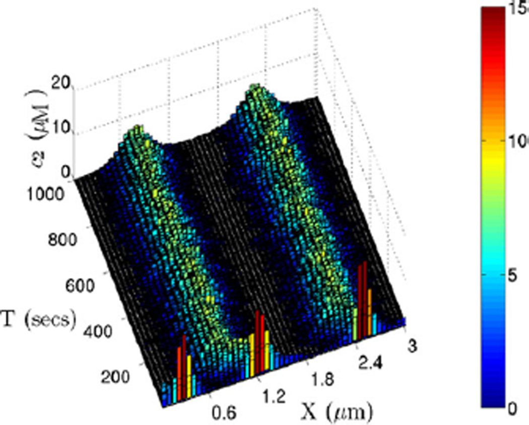
If we further increase the cross-section to 0.9 × 0.9 µm2, the stochastic simulation always approaches the same stable non-uniform steady state as shown in Fig. 23. The deterministic prediction in Fig. 19 shows that different initial conditions drive the system into different steady states, but the stochastic simulation always evolves to a distribution corresponding to that obtained from the PDE with non-zero initial condition. This indicates that even with zero initial conditions the intrinsic fluctuations are large enough to drive the system to this stationary distribution.
Fig. 23.
The evolution of one realization of the RD system with parameter set 3. The domain of size (3, 0.9, 0.9) µm is divided into 50 cells along the x-axis, and with this choice the stochastic simulations always converge to the same distribution, which is also a deterministic solution of the PDE
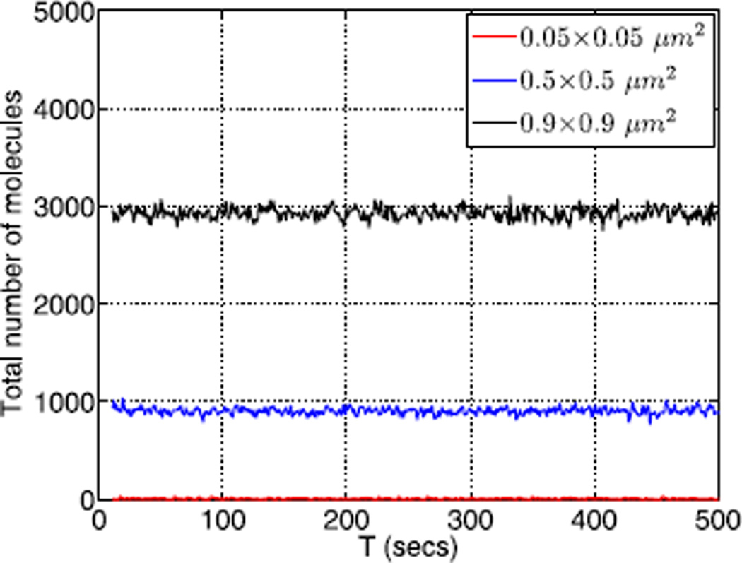
In these simulations we have assumed that the distributions on a cross-section are uniform, and we find that as the cross-section increases the solution of the stochastic problem resembles a solution of the PDE more reliably. On the smallest cross section of 0.05 × 0.05 µm2, the dynamics of the system wanders ‘aimlessly’, whereas on a larger cross section of 0.5 × 0.5 µm2 we observe more persistent wandering between limited numbers of stationary distributions. With an even larger cross section of 0.9 × 0.9 µm2, the dynamics always leads to one stationary distribution. The underlying reason for this progression is simple: we scale coefficients with the volume, which leads to a larger amount of molecules, and thus the stochastic simulation corresponds more closely with the PDE version of the system dynamics. Particularly for the glycolytic system, which has several coexisting steady states, the smaller the cross section is, the larger the fluctuations in the numbers of molecules in individual compartments. The evolution of the total number of molecules for these different cross sections is depicted in Fig. 24.
Fig. 24.
The temporal evolution of the total number of second component of the glycolytic system for three different cross section sizes of the domain as in Figs. 21–23. The mean of the total number of molecules in the whole domain for three cross sections from least to largest are 9.01, 902.4, 2925.4, respectively, whereas the variances are 0.647, 0.037, 0.02
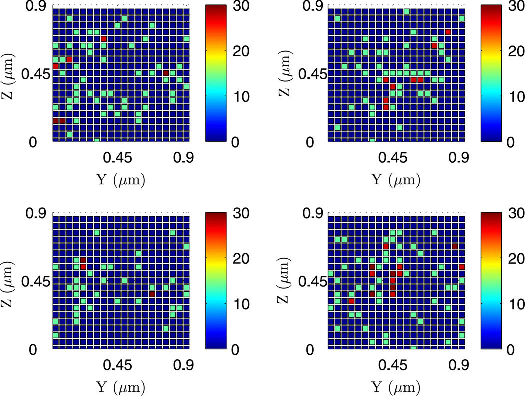
One limitation of the larger cross-section is that the compartment width in the y-and z-directions may exceed the maximal compartment size, and thereby invalidate the stochastic simulation. In other words, the real dynamics in the full 3D system with the same large cross section may show a non-uniform distribution of species in the y–z plane, under which the assumption of a well-mixed cross section is no longer appropriate. To demonstrate this, we used the optimized algorithm to do a stochastic simulation of the full 3D system similar to the above, but further divided the 0.9 × 0.9 µm2 cross section into 20 × 20 compartments. First, we examine the averaged concentration of the cross section along the x-axis. The result in Fig. 25 shows a temporally changing dynamics in the pattern which is quite different from that in Fig. 23. Interestingly, the averaged cross-sectional concentrations shown there occasionally resemble the non-uniform steady states predicted by the PDE, but detailed plots of the species concentration on various cross sections along the x-axis show that the cross sections are clearly not well-mixed (cf. Fig. 26). Thus the assumption of well-mixed species for the large cross-sections is not valid in this system. We also extracted the dynamics of the compartments with same y–z position along the x-axis as depicted in Fig. 27, and found that the dynamics along these fibers show no clear patterns close to the steady state predicted by the PDE. In fact they resemble the earlier results on a small cross section more closely.
Fig. 25.
The evolution of one realization of the glycolytic RD system with parameter set 3. The domain of size (3, 0.9, 0.9) µm has 50, 20 and 20 divisions in the x-, y- and z-directions, respectively. Shown are the dynamics in different time intervals, and the concentration in any y–z plane is averaged and projected to the x-axis
Fig. 26.
The dynamics on four cross-sections along the x-axis extracted from the full 3D dynamics at t = 1000 s. The x-coordinates are 0.6, 1.2, 1.8, 2.4 µm, respectively
Fig. 27.
Dynamics in two fibers of compartments along the x-axis extracted from the full 3D dynamics of the glycolytic reactions. The left fiber has coordinates (y, z) = (0.45, 0.45), whereas the right is (y, z) = (0.9, 0.9)
5.4 Conclusion
Stochastic simulations of RD systems raise a number of issues that must be confronted in evaluating the results. First is how one can determine the appropriate compartment size, and given that, how to deal with the increased computational complexity of distributed systems. We have given several criteria that can be used for the former, and have developed a new computational algorithm that optimizes the search process in a Gillespie algorithm. Our comparison of predictions from the PDE with those from stochastic simulations of the 1D system shows that the choice of the computational cell size is critical, and that results obtained using a sufficiently small size may bear little relation to the deterministic results when there are multiple solutions. In that case the dynamics of the stochastic simulation may wander between these steady states, with the residence time in each depending on the size of the attraction basin. This is less of a problem when the PDE has a unique attractor, but spatial non-uniformity may still lead to significant differences in the predicted behavior when the number of molecules is low.
Acknowledgements
Research supported in part by Grant # GM 29123 from the National Institutes of Health, and in part by the Mathematical Biosciences Institute and the National Science Foundation under grant DMS 0931642.
Footnotes
Other scalings may be applicable in other regimes, but would lead to different evolution equations (Hillen and Othmer 2000).
These estimates are predicated on a uniform distribution of species in the compartments. They could be very different if there are spatial gradients, but estimates are difficult in that case.
Here and hereafter we assume that block sizes are chosen so that Nc is a multiple of m.
Contributor Information
Jifeng Hu, School of Mathematics, University of Minnesota, Minneapolis, MN 55455, USA.
Hye-Won Kang, Mathematical Biosciences Institute, Ohio State University, Columbus, OH, USA.
Hans G. Othmer, Email: othmer@math.umn.edu, School of Mathematics and Digital Technology Center, University of Minnesota, Minneapolis, MN 55455, USA.
References
- Agbanusi IC, Isaacson SA. A comparison of bimolecular reaction models for stochastic reaction diffusion models. 2013 doi: 10.1007/s11538-013-9833-6. arXiv: 1301.0547. [DOI] [PubMed] [Google Scholar]
- Ander M, Beltrao P, Di Ventura B, Ferkinghoff-Borg J, Foglierini M, Kaplan A, Lemerle C, Tomas-Oliveira I, Serrano L. SmartCell, a framework to simulate cellular processes that combines stochastic approximation with diffusion and localisation: analysis of simple networks. Syst. Biol. 2004;1(1):129–138. doi: 10.1049/sb:20045017. [DOI] [PubMed] [Google Scholar]
- Applebaum D. Lévy processes and stochastic calculus. Vol. 93. Cambridge: Cambridge University Press; 2004. [Google Scholar]
- Arnold L. Stochastic differential equations, theory and applications. New York: Wiley-Interscience; 1974. [Google Scholar]
- Ashkenazi M, Othmer HG. Spatial patterns in coupled biochemical oscillators. J. Math. Biol. 1978;5:305–350. [Google Scholar]
- Bernstein D. Simulating mesoscopic reaction–diffusion systems using the Gillespie algorithm. Phys. Rev. E. 2005;71(4 Pt 1) doi: 10.1103/PhysRevE.71.041103. 041103. [DOI] [PubMed] [Google Scholar]
- Callen HB. Thermodynamics. New York: Wiley; 1960. [Google Scholar]
- Cao Y, Li H, Petzold L. Efficient formulation of the stochastic simulation algorithm for chemically reacting systems. J. Chem. Phys. 2004;121(9):4059–4067. doi: 10.1063/1.1778376. [DOI] [PubMed] [Google Scholar]
- Capasso V, Bakstein D. An introduction to continuous-time stochastic processes: theory, models, and applications to finance, biology, and medicine. New York: Birkhauser; 2005. [Google Scholar]
- Chueh KN, Conley CC, Smoller JA. Positively invariant regions for systems of nonlinear diffusion equations. Indiana University Math. J. 1977;26(2):373–392. [Google Scholar]
- Conway E, Hoff D, Smoller J. Large time behavior of solutions of systems of nonlinear reaction–diffusion equations. SIAM J. Appl. Math. 1978;35(1):1–16. [Google Scholar]
- Elf J, Ehrenberg M. Spontaneous separation of bi-stable biochemical systems into spatial domains of opposite phases. IET Syst. Biol. 2004;1:230–236. doi: 10.1049/sb:20045021. [DOI] [PubMed] [Google Scholar]
- Erban R, Othmer H. From signal transduction to spatial pattern formation in E. coli: a paradigm for multi-scale modeling in biology. Multiscale Model. Simul. 2005;3(2):362–394. [Google Scholar]
- Erban R, Othmer HG. Taxis equations for amoeboid cells. J. Math. Biol. 2007;54(6):847–885. doi: 10.1007/s00285-007-0070-1. [DOI] [PubMed] [Google Scholar]
- Gadgil C, Lee CH, Othmer HG. A stochastic analysis of first-order reaction networks. Bull. Math. Biol. 2005;67:901–946. doi: 10.1016/j.bulm.2004.09.009. [DOI] [PMC free article] [PubMed] [Google Scholar]
- Gibson MA, Bruck J. Efficient exact stochastic simulation of chemical systems with many species and many channels. J. Phys. Chem. A. 2000;104:1876–1889. [Google Scholar]
- Gierer A, Meinhardt H. A theory of biological pattern formation. Biol. Cybern. 1972;12(1):30–39. doi: 10.1007/BF00289234. [DOI] [PubMed] [Google Scholar]
- Gillespie DT. Exact stochastic simulation of coupled chemical reactions. J. Phys. Chem. 1977;81(25):2340–2361. [Google Scholar]
- Hillen T, Othmer HG. The diffusion limit of transport equations derived from velocity jump processes. SIAM J. Appl. Math. 2000;61:751–775. [Google Scholar]
- Isaacson SA. The reaction–diffusion master equation as an asymptotic approximation of diffusion to a small target. SIAM J. Appl. Math. 2009;70(1):77–111. [Google Scholar]
- Kang HW, Zheng L, Othmer HG. A new method for choosing the computational cell in stochastic reaction–diffusion systems. J. Math. Biol. 2012;65:1017–1099. doi: 10.1007/s00285-011-0469-6. [DOI] [PMC free article] [PubMed] [Google Scholar]
- Kang HW, Zheng L, Othmer HG. The effect of the signalling scheme on the robustness of pattern formation in development. Interface Focus. 2012;2(4):465–486. doi: 10.1098/rsfs.2011.0116. [DOI] [PMC free article] [PubMed] [Google Scholar]
- Li H, Petzold L. Logarithmic direct method for discrete stochastic simulation of chemically reacting systems (Technical Report) Santa Barbara: Department of Computer Science, University of California; 2006. [Google Scholar]
- Matzavinos A, Othmer HG. A stochastic analysis of actin polymerization in the presence of twinfilin and gelsolin. J. Theor. Biol. 2007;249:723–736. doi: 10.1016/j.jtbi.2007.08.018. [DOI] [PubMed] [Google Scholar]
- Metzler R, Klafter J. The random walk’s guide to anomalous diffusion: a fractional dynamics approach. Phys. Rep. 2000;339(1):1–77. [Google Scholar]
- Othmer HG. Nonuniqueness of equilibria in closed reacting systems. Chem. Eng. Sci. 1976;31:993–1003. [Google Scholar]
- Othmer HG. Some mathematical questions in biology. Vol. VIII. Providence: Am. Math. Soc.; 1977. Current problems in pattern formation; pp. 57–85. [Google Scholar]
- Othmer HG, Dunbar SR, Alt W. Models of dispersal in biological systems. J. Math. Biol. 1988;26:263–298. doi: 10.1007/BF00277392. [DOI] [PubMed] [Google Scholar]
- Othmer HG, Aldridge JA. The effects of cell density and metabolite flux on cellular dynamics. J. Math. Biol. 1978;5:169–200. doi: 10.1007/BF00275897. [DOI] [PubMed] [Google Scholar]
- Othmer HG, Xue C. The mathematical analysis of biological aggregation and dispersal: progress, problems and perspectives. In: Lewis M, Maini P, Petrovskii S, editors. Dispersal, individual movement and spatial ecology: a mathematical perspective. Heidelberg: Springer; 2013. [Google Scholar]
- Prigogine I, DeFay R. Chemical thermodynamics. New York: Longmans, Green; 1954. [Google Scholar]
- Sato KI. Lévy processes and infinitely divisible distributions. Cambridge: Cambridge University Press; 1999. [Google Scholar]
- Shimmi O, O’Connor MB. Physical properties of Tld, Sog, Tsg and Dpp protein interactions are predicted to help create a sharp boundary in Bmp signals during dorsoventral patterning of the Drosophila embryo. Development. 2003;130(19):4673–4682. doi: 10.1242/dev.00684. [DOI] [PubMed] [Google Scholar]
- Tomioka R, Kimura H, Kobayashi TJ, Aihara K. Multivariate analysis of noise in genetic regulatory networks. J. Theor. Biol. 2004;229(4):501–521. doi: 10.1016/j.jtbi.2004.04.034. [DOI] [PubMed] [Google Scholar]
- Turing AM. The chemical basis of morphogenesis. Philos. Trans. R. Soc. Lond. B, Biol. Sci. 1952;237:37–72. doi: 10.1098/rstb.2014.0218. [DOI] [PMC free article] [PubMed] [Google Scholar]
- Umulis DM, Othmer HG. Mechanisms of scaling in spatial pattern formation. Development. 2013 doi: 10.1242/dev.100511. (to appear). [DOI] [PMC free article] [PubMed] [Google Scholar]
- Weiss GH. Aspects and applications of the random walk. Amsterdam: North-Holland; 1994. [Google Scholar]
- Wilemski G. On the derivation of Smoluchowski equations with corrections in the classical theory of Brownian motion. J. Stat. Phys. 1976;14(2):153–169. [Google Scholar]
- Xue C, Othmer HG. Multiscale models of taxis-driven patterning in bacterial populations. SIAM J. Appl. Math. 2009;70(1):133–167. doi: 10.1137/070711505. [DOI] [PMC free article] [PubMed] [Google Scholar]
- Xue C, Budrene EO, Othmer HG. Radial and spiral stream formation in Proteus mirabilis colonies. PLoS Comput. Biol. 2011;7(12):e1002332. doi: 10.1371/journal.pcbi.1002332. [DOI] [PMC free article] [PubMed] [Google Scholar]


