Computing Smooth Time-Trajectories for Camera and Deformable Shape in Structure from Motion with Occlusion

Abstract

We address the classical computer vision problems of rigid and non-rigid structure from motion (SFM) with occlusion. We assume that the columns of the input observation matrix W describe smooth 2D point trajectories over time. We then derive a family of efficient methods that estimate the column space of W using compact parameterizations in the Discrete Cosine Transform (DCT) domain. Our methods tolerate high percentages of missing data and incorporate new models for the smooth time-trajectories of 2D-points, affine and weak-perspective cameras, and 3D deformable shape. We solve a rigid SFM problem by estimating the smooth time-trajectory of a single camera moving around the structure of interest. By considering a weak-perspective camera model from the outset, we directly compute Euclidean 3D shape reconstructions without requiring post-processing steps such as Euclidean upgrade and bundle adjustment. Our results on real SFM datasets with high percentages of missing data were positively compared to those in the literature. In non-rigid SFM, we propose a novel 3D shape trajectory approach that solves for the deformable structure as the smooth time-trajectory of a single point in a linear shape space. A key result shows that, compared to state-of-the-art algorithms, our non-rigid SFM method can better model complex articulated deformation with higher frequency DCT components while still maintaining the low-rank factorization constraint. Finally, we also offer an approach for non-rigid SFM when W is presented with missing data.

1 INTRODUCTION

Accurately describing a data matrix as a product of two low-rank factors, matrix factorization, is a fundamental task in computer vision and pattern recognition. This paper focuses on the classical computer vision problem of matrix factorization in rigid and non-rigid structure from motion (SFM) [5], [29]. The goal in SFM is to jointly estimate the 3D scene structure and relative camera motion from corresponding 2D points in a sequence of images. Applications of SFM include autonomous navigation, image augmentation, and the construction of rigid and deformable 3D models from images [11], [15]. The modeling of deformable shapes such as the human hand, face, and body is also of particular importance in computer graphics, and human-computer interaction (e.g., [10]).

While techniques for rigid SFM have matured considerably over the past two decades [6]-[8], [12], [16], [17], [19], [21], [28], non-rigid SFM is still a very difficult problem, especially for complex articulated deformations [30]. The difficulty in providing good solutions reflects the underconstrained nature of SFM once the rigidity assumption is removed. Recent research has thus focused on the definition of new constraints (priors) to solve this problem [1]-[3], [23], [24], [26], [30], [32]-[34].

In the standard matrix factorization approach to SFM [5], [29], each column of the input matrix $\mathrm{W}\in {\mathbb{R}}^{m\times n}$ has a sequence of 2D coordinates of the same 3D structure point as observed from different locations. Considering W of a predefined low-rank r ≤ min(m, n), the SFM solution is obtained from the factorization

$$\mathrm{W}=\mathrm{MS},\mathrm{M}\in {\mathbb{R}}^{m\times r},\mathrm{S}\in {\mathbb{R}}^{r\times n}.$$ (1)

In rigid SFM, r = 4 and S describes the 3D shape observed by the cameras in M. In non-rigid SFM, each observed shape of the deformable structure is represented in a linear shape space defined by K basis shapes in S. Then, r = 3K + 1 and M includes the cameras and also the shape coordinates in terms of basis S. In both cases, factors M and S may be obtained from the singular value decomposition (SVD) of W. In practice, however, a large portion of the 2D observations in W is often missing because of occlusions. Therefore, standard matrix factorization algorithms such as SVD [13] cannot be directly used. To solve SFM, it is also necessary to overcome other challenges such as tracking errors [19] and degeneracies in the assumed camera motion and shape deformation – i.e., when the above constraints on the rank r of W do not hold [21], [32], [34].

To compute more accurate and efficient solutions to rigid and non-rigid SFM with occlusion, we start by assuming that each column of W represents the smooth time-trajectory of a 2D point. Such 2D trajectories are usually provided by a feature tracking algorithm that operates on a monocular video sequence. Equivalently, we assume that the 2D observations were obtained by a single camera moving smoothly around the structure of interest (Fig. 1). Our factorization approach tolerates missing data and defines constraints that considerably reduce the number of unknowns that need to be estimated. First, we consider factor S only implicitly, reformulating the factorization problem in terms of M alone. Second, because M is a basis for the smooth 2D trajectories in the columns of W, we solve for a compact representation of M in a subspace of the Discrete Cosine Transform (DCT) basis vectors. Our algorithms are remarkably efficient in cases of long image sequences and many imaged points (i.e., when W has high-dimensional column and row spaces).

Fig. 1.

The smooth trajectory (dashed line) of a single camera moving around the structure of interest (cube) over time (t).

We solve for rigid SFM by estimating only the smooth time-trajectory of a camera’s projection plane, Fig. 1. Also, by considering the weak-perspective camera model from the outset, we directly solve for Euclidean shape and cameras. Therefore, our method does not require post-processing algorithms that upgrade and refine the initial affine solution (e.g., bundle adjustment [15]).

In non-rigid SFM, we assume that the smooth 2D trajectories in W also reflect the smooth deformation of the observed 3D structure over time. The deformable structure is represented as a single point moving smoothly in a linear shape space, Fig. 2. We then solve for a single, smooth 3D shape trajectory with time-coordinates in factor M. Thus, the associated basis shapes are defined only implicitly in factor S. Once M has been estimated, S is then trivially computed from M and W by solving simple linear systems of equations.

Fig. 2.

The smooth time-trajectory (dashed line) of a deforming 3D shape (cube). The object shape is represented by a single point (blue sphere) with coordinates relative to 3D basis shapes Ŝ₁, Ŝ₂, and Ŝ₃ (not shown). As the shape deforms smoothly over time (t), its point representation describes a single, smooth 3D shape trajectory.

Our work is most closely related to the recent non-rigid SFM method by Akhter et al. [2]. They propose a factorization approach that does not define a linear shape space, but recovers instead independent 3D point trajectories over time. The DCT vectors are used as a basis for individual 3D point trajectories. Their method has provided some of the best results on highly articulated shapes to date. However, the main problem is the method’s inability to use additional, higher frequency DCT vectors without increasing the rank of the resulting matrix factors. Thus, its application is restricted to structures with slow and smooth deformation. The method does not address the missing data problem either; W is assumed complete and factorized using SVD.

In this paper, we also present an interpretation of Akhter et al.’s approach in terms of a linear shape space and show that their results correspond to coarse approximations of our solutions. Our non-rigid SFM method provides better results on complex articulated deformations due to its more effective use of higher-frequency DCT components without increasing the factorization rank. Furthermore, we use the DCT basis to model a camera’s trajectory and efficiently solve for rigid SFM. Finally, we also contribute with missing data approaches for both rigid and non-rigid SFM.

One main group of related methods that address the missing data problem are known as batch algorithms [14], [17], [19], [23], [28]. These methods propose strategies for combining partial rank-r factorizations obtained for complete sub-blocks of W. Examples include the subspace constraint algorithms that reconstruct W by first building its row null-space [17], [19], column null-space [14], [23], or one of its range spaces [28]. The main problem with these methods is their sub-optimality since errors in the factorization of sub-blocks are propagated to the subsequent optimization stage. Also, the rank-r constraint may not apply to all sub-blocks in case of degenerate motion and deformation [21], [23].

A second group of missing data approaches include iterative methods that use all data at once without searching for complete sub-blocks in W [6], [8], [16], [24], [30], [31]. Among these, alternation methods [16], [24], [30] iteratively solve for subsets of unknowns while the others remain fixed. For instance, PowerFactorization [16] solves for factors M and S in a simple, alternated least-squares manner. It presents very slow convergence when a considerable amount of data is missing. However, the method is useful in initializing faster Newton methods [6] that minimize matrix fitting error in terms of M and S. The Levenberg-Marquardt-Subspace (LM-S) method in [8] considers S as an implicit function of M and W and solves for M only. Despite its superior performance, proper initialization of this method remains an open problem. The method’s complexity also makes it difficulty to integrate additional constraints into the factorization problem.

In the following, we present our Column Space Fitting (CSF) method that computes a rank-r basis M for the column space of a matrix with missing data. Using a simple Gauss-Newton-based approximation to the Hessian matrix, our method provides equivalent or better solutions for M when compared to LM-S on matrices with high percentage of missing data. Furthermore, the simplicity of our approach allows us to easily consider additional constraints in the factorization problem, such as a mean column vector and a pre-defined reference basis for M. We then solve for a compact representation of M in a subspace defined in terms of the DCT basis vectors. As a result, we offer a family of CSF algorithms for rigid and non-rigid SFM problems. Our methods always start from a deterministic initialization corresponding to a “coarse” solution for M.

This paper is organized as follows. Section 2 derives our general CSF approach for matrix factorization with missing data. In Section 3, we solve for rigid SFM by estimating a smooth time-trajectory of an affine or a weak-perspective camera. Section 4 describes our 3D shape trajectory approach to non-rigid SFM. Sections 5 and 6 present experimental results and conclusion.

2 Solving for the Column Space of a Matrix with Missing Data

We formulate the rank-r factorization of incomplete matrix W as solving exclusively for a column space basis M of rank-r. To facilitate the introduction of additional constraints into the factorization procedure, especially in SFM problems, we first derive our Column Space Fitting (CSF) algorithm. We then show how to solve for M in the subspace spanned by a predefined bases. When such a bases is defined in terms of the DCT basis vectors, we propose a simple, deterministic initial form of M.

2.1 General CSF approach

Consider $\mathrm{W}\in {\mathbb{R}}^{m\times n}$ as in (1) and note the related equation S = M^†W, where † denotes the Moore-Penrose pseudo-inverse [13].

Assuming W is presented with missing data, let the complete vector ${\mathrm{w}}_j\in {\mathbb{R}}^{m_j}(m_j\le m)$ denote all the observed entries in the j^th column of W. Also, define ${\Pi }_j\in {\mathbb{R}}^{m_j\times m}$ as a row-amputated identity matrix such that M_j = Π_jM has the rows in M that correspond to the rows of entries in w_j. Then w_j = M_js_j, with the complete j^th column of S defined as ${\mathrm{s}}_j={\mathrm{M}}_j^{†}{\mathrm{w}}_j\in {\mathbb{R}}^r$.

The goal is to minimize

$$f\left(\mathrm{M}\right)=\frac{1}{2}\sum _j{\mid \mid \left(\mathrm{I}-{\mathrm{M}}_j{\mathrm{M}}_j^{†}\right){\mathrm{w}}_j\mid \mid }_F^2,$$ (2)

where ∥·∥_F is the Frobenius norm. To better understand the meaning of (2), let the projector on the orthogonal space of M_j be

$${\mathrm{P}}_j^{\perp }=\left(\mathrm{I}-{\mathrm{M}}_j{\mathrm{M}}_j^{†}\right)\in {\mathbb{R}}^{m_j\times m_j}.$$ (3)

Rewriting (2) in terms of residual (error) vectors ${\mathrm{r}}_j\in {\mathbb{R}}^{m_j}$, we have

$$f\left(\mathrm{M}\right)=\frac{1}{2}\sum _j{\mathrm{r}}_j^T{\mathrm{r}}_j,{\mathrm{r}}_j={\mathrm{P}}_j^{\perp }{\mathrm{w}}_j.$$ (4)

Algorithm 1.

Column Space Fitting (CSF) method for minimizing the error function f (M).

1: M ← initial matrix (M0).

2: δ ← initial damping scalar (δ0).

3: repeat

4: Compute gradient (g) and Hessian (H) from Jacobian terms (Jj).

5: repeat

6: δ ← δ × 10.

7: Find ΔM from vec (ΔM) ← (H + δI)−1g.

8: until f (M− ΔM) < f (M).

9: M ← M − ΔM.

10: δ ← δ × 10−2.

11: Orthogonalize M (keep mean vector t unchanged).

12: until convergence.

Therefore, we minimize the overall matrix fitting error as defined by a sum of squared Euclidean distances from each observed column vector to the subspace spanned by the corresponding rows in M.

The error function (2) is minimized using our Column Space Fitting (CSF) method, based on Levenberg-Marquardt optimization [4], which we summarize in Algorithm 1. M is first set to an initial matrix. Then, in each iteration, we update the current estimate of M by computing an adjustment matrix ΔM in vectorized form, vec(ΔM), which stacks the columns of ΔM in a single vector of unknowns. We solve for vec(ΔM) using the gradient vector (g) and Hessian matrix (H) of f as given by matrix differential calculus [20]. The damping parameter δ leads to combined Gauss-Newton and steepest-descent iterations when H becomes singular. For numerical stability, we orthogonalize M at the end of each iteration.

To compute g and H, we follow a Gauss-Newton-based derivation in terms of Jacobian matrices J_j for each vector w_j (see complete derivation in Appendix A). The first and second differentials of f(M) are

$$df=-\sum _j{\left({\mathrm{J}}_j^T{\mathrm{r}}_j\right)}^{T}vec\left(d\mathrm{M}\right),$$ (5)

$$d^{2}f=\sum _{j}vec{\left(d\mathrm{M}\right)}^T\left({\mathrm{J}}_j^T{\mathrm{J}}_j\right)vec\left(d\mathrm{M}\right),$$ (6)

$${\mathrm{J}}_j={\mathrm{s}}_j^T\otimes {\mathrm{P}}_j^{\perp }{\Pi }_j.$$ (7)

In (7), ⊗ is the Kronecker product and ${\mathrm{s}}_j={\mathrm{M}}_j^{†}{\mathrm{w}}_j$ denotes the current (and implicit) estimate of the j^th column of factor S. From (5) and (6), we identify

$$\mathrm{g}=-\sum _j{\mathrm{J}}_j^T{\mathrm{r}}_j\text{and}\mathrm{H}=\sum _j{\mathrm{J}}_j^T{\mathrm{J}}_j.$$ (8)

For comparison, the forms of g and H as computed in [8] are reproduced in our supplementary documentation file. It is important to note that the simplicity of our expressions above makes it easier to consider additional optimization constraints as described next.

As an alternative to the derivations given above, we can solve for rank-(r − 1) factors M and S, and an additional mean column $\mathrm{t}\in {\mathbb{R}}^m$ such that W = MS + t1^T , where $1\in {\mathbb{R}}^n$ is a vector of all ones. This is a very useful model in applications such as rigid and non-rigid SFM. Equivalently, we solve for a rank-r factorization

$$\mathrm{W}=\tilde{\mathrm{M}}\tilde{\mathrm{S}}=\left[\mathrm{M}\mathrm{t}\right]\left[\begin{array}{c}\hfill \mathrm{S}\hfill \\ \hfill 1^T\hfill \end{array}\right],$$ (9)

with extended factors M̃ and S̃. The mean column interpretation for the last column of M̃ constrains the last row of S̃ to be 1^T. Therefore, the model in (9) has fewer degrees of freedom than that in (1) and the final matrix fitting error, f(M̃), is expected to be higher.

The goal now is to minimize

$$f(\mathrm{M},\mathrm{t})=\frac{1}{2}\sum _j{\mathrm{r}}_j^T{\mathrm{r}}_j,{\mathrm{r}}_j={\mathrm{P}}_j^{\perp }(w_j-{\mathrm{t}}_j),$$ (10)

with t_j = Π_jt and ${\mathrm{P}}_j^{\perp }$ computed from M_j only. The new Jacobian terms are then derived for vec(dM̃) as

$${\mathrm{J}}_j=\left[{\mathrm{s}}_j^{T}1\right]\otimes {\mathrm{P}}_j^{\perp }{\Pi }_j,$$ (11)

with ${\mathrm{s}}_j={\mathrm{M}}_j^{†}({\mathrm{w}}_j-{\mathrm{t}}_j)$ (see derivation in Appendix A).

In this case, at the end of each iteration, only the left-most r − 1 columns of M̃ are orthogonalized and t is kept unchanged.

2.2 Solution with a predefined basis

Let the columns of a matrix $\mathrm{B}\in {\mathbb{R}}^{m\times d}$ contain a predefined set of basis vectors (e.g., a truncated DCT basis). We now consider a factor M of the form

$$\mathrm{M}=\mathrm{BX},\mathrm{X}\in {\mathbb{R}}^{d\times r}.$$

Each column of X has d ≤ m coordinates for the corresponding column of M as represented in the d-dimensional space spanned by B.

Previously, we had implicitly considered a canonical basis B = I_m, the m × m identity matrix, and solved for X = M. Now, in each iteration we solve for the update step vec(dX) with gradient and Hessian as in (8). The Jacobian terms are given by

$${\mathrm{J}}_j={\mathrm{s}}_j^T\otimes {\mathrm{P}}_j^{\perp }{\Pi }_j\mathrm{B}.$$ (12)

It is important to describe our motivation for using a predefined basis: Problems in different application domains involve matrices (W) whose columns have observations of random variables that change only gradually over time. Observations in each column can be considered as samples of a smooth signal over time with a narrow bandwidth spectrum in the DCT domain. This means that most of the energy of a signal (column) is captured by a small number of low-frequency DCT components, leading to a compact representation X (i.e., small d).

In the next sections, we consider matrices B constructed from DCT basis vectors, with the right-most columns corresponding to higher-frequency components. Since signal smoothness leads to high-frequency coefficients close to zero, we propose an initialization of X, denoted X₀, of the form

$${\mathrm{X}}_0=\left[\begin{array}{c}\hfill \mathrm{Q}\hfill \\ \hfill 0\hfill \end{array}\right],\mathrm{Q}\in {\mathbb{R}}^{r\times r}.$$

The goal becomes initializing a small block Q, which must be full-rank (i.e., the rank of M = BX₀ is rank(Q)). For any full-rank Q, an equally good initial solution is given by the simple and deterministic initialization

$${\mathrm{X}}_0=\left[\begin{array}{c}\hfill \mathrm{Q}\hfill \\ \hfill 0\hfill \end{array}\right]{\mathrm{Q}}^{-1}=\left[\begin{array}{c}\hfill {\mathrm{I}}_r\hfill \\ \hfill 0\hfill \end{array}\right].$$ (13)

As a proof, we note that the factorization in (1) is defined only up to a rank-r ambiguity matrix Q such that W = MS = (MQ⁻¹)(QS).

As a result, we can even fix the values for the topmost block of X as I_r and solve only for the remaining (d − r) × r submatrix. Note that (d − r)r is the number of parameters defining an r-dimensional linear space embedded in another d-dimensional linear space.

When the last column of X is interpreted as the coefficients of the mean column vector t, the ambiguity matrix Q is of rank (r − 1) only, i.e., the last row of S is constrained to be 1^T. This fact suggests to initialize the last column of X with zeros (t = 0).

3 Rigid SFM: Estimating the Smooth Time-Trajectory of a Camera

This section focuses on rigid SFM with occlusion. We assume the point tracks in W were obtained from a monocular video sequence provided by a single, smoothly moving camera. First, we present a method using a compact DCT basis to represent the smooth trajectory of a general affine camera. Subsequently, we further improve on this method by using a weak-perspective camera model from the outset to directly estimate Euclidean cameras and shape. Once the final solution for M is defined, each column s_j of S is obtained independently as in the computation of the Jacobian terms above.

3.1 Affine camera trajectory

In rigid SFM with T images, $\mathrm{W}\in {\mathbb{R}}^{2T\times n}$ is

$$\mathrm{W}=\left[\begin{array}{ccc}\hfill x_{11}\hfill & \hfill \dots \hfill & \hfill x_{1n}\hfill \\ \hfill y_{11}\hfill & \hfill \dots \hfill & \hfill y_{1n}\hfill \\ \hfill ⋮\hfill & \hfill \hfill & \hfill ⋮\hfill \\ \hfill x_{T1}\hfill & \hfill \dots \hfill & \hfill x_{Tn}\hfill \\ \hfill y_{T1}\hfill & \hfill \dots \hfill & \hfill y_{Tn}\hfill \end{array}\right]=\mathrm{M}\left[\begin{array}{ccc}\hfill {\mathrm{s}}_1\hfill & \hfill \dots \hfill & \hfill {\mathrm{s}}_n\hfill \\ \hfill 1\hfill & \hfill \hfill & \hfill 1\hfill \end{array}\right],$$ (14)

with [x_tj, y_tj]^T the 2D projection of 3D point s_j in the t^th image (t = 1, 2, … , T; j = 1, 2, … , n). Here, the motion factor $\mathrm{M}\in {\mathbb{R}}^{2T\times 4}$ describes a stack of T affine camera matrices $\widehat{{\mathrm{M}}_t}\in {\mathbb{R}}^{2\times 4}$,

$$\mathrm{M}=\left[\begin{array}{c}\hfill {\widehat{\mathrm{M}}}_1\hfill \\ \hfill ⋮\hfill \\ \hfill {\widehat{\mathrm{M}}}_T\hfill \end{array}\right],{\widehat{\mathrm{M}}}_t=\left[{\widehat{\mathrm{A}}}_t{\widehat{\mathrm{t}}}_t\right],$$ (15)

where ${\widehat{\mathrm{A}}}_t\in {\mathbb{R}}^{2\times 3}$ is a general affine projection and ${\widehat{\mathrm{t}}}_t\in {\mathbb{R}}^2$ is a 2D translation. The rows of ${\widehat{\mathrm{A}}}_t$ are 3D vectors defining the x and y axes (not necessarily orthonormal) of the camera’s projection plane in the t^th observation.

Assuming the 8 camera parameters vary smoothly over time, we define the camera as a sample of a smooth matrix function of time, ${\widehat{\mathrm{M}}}_t=\widehat{\mathrm{M}}\left(t\right)$. We then parameterize $\widehat{\mathrm{M}}\left(t\right)$ using 8 independent cosine series whose f^th frequency coefficients are given in ${\widehat{\mathrm{X}}}_f\in {\mathbb{R}}^{2\times 4}$,

$${\widehat{\mathrm{M}}}_t=\left[\widehat{\mathrm{A}}\left(t\right)\widehat{\mathrm{t}}\left(t\right)\right]=\sum _{f=1}^d{\omega }_{tf}{\widehat{\mathrm{X}}}_f.$$ (16)

Each constant ω_tf above is the f^th frequency cosine term at time t,

$${\omega }_{tf}=\frac{{\sigma }_f}{\sqrt{T}}\cos \left(\frac{\pi (2t-1)(f-1)}{2T}\right),$$

with σ₁ = 1 and, for $f\ge 2,{\sigma }_f=\sqrt{2}$.

The goal is then to solve for d ≤ T matrices ${\widehat{\mathrm{X}}}_f$ . Let ${\Omega }_d\in {\mathbb{R}}^{T\times d}$ be a truncated, orthonormal DCT matrix whose (t; f)^th entry is ω_tf, as above. Substituting (16) into (15) yields

$$\mathrm{M}=({\Omega }_d\otimes {\mathrm{I}}_2)\left[\begin{array}{c}\hfill {\widehat{\mathrm{X}}}_1\hfill \\ \hfill ⋮\hfill \\ \hfill {\widehat{\mathrm{X}}}_d\hfill \end{array}\right]={\mathrm{B}}_{af}\mathrm{X}.$$

Thus, with basis ${\mathrm{B}}_{af}=({\Omega }_d\otimes {\mathrm{I}}_2)\in {\mathbb{R}}^{2T\times 2d}$, we solve for $\mathrm{M}\in {\mathbb{R}}^{2T\times 4}$ as a function of $\mathrm{X}\in {\mathbb{R}}^{2d\times 4}$. Note that the smoothness assumption implies d ⪡ T. We solve for X as in Section 2.2, with extended terms ${\tilde{\mathrm{s}}}_j^T=\left[{\mathrm{s}}_j^{T}1\right]$ in (12).

For simplicity, and unless stated otherwise, we assume in this paper that the number of DCT components d has been fixed a priori based on empirical observations (e.g., expected motion or noise level). An alternative coarse-to-fine strategy can start with a small d and increment its value until a convergence criterion is verified. For instance, d can be incremented until the energy of the highest frequency coefficients falls below a small percentage p_d ∈ (0, 1) of the total energy,

$${\mid \mid {\mathrm{x}}_d^T\mid \mid }_F<p_d{\mid \mid \mathrm{X}\mid \mid }_F,$$

where ${\mathrm{x}}_d^T$ is the last row of X.

$${\widehat{\mathrm{R}}}_t={\lambda }_t\left[\begin{array}{ccc}\hfill \cos {\alpha }_t\cos {\beta }_t\cos {\gamma }_t-\sin {\alpha }_t\sin {\gamma }_t\hfill & \hfill -\cos {\alpha }_t\cos {\beta }_t\sin {\gamma }_t-\sin {\alpha }_t\cos {\gamma }_t\hfill & \hfill \cos {\alpha }_t\sin {\beta }_t\hfill \\ \hfill \sin {\alpha }_t\cos {\beta }_t\cos {\gamma }_t+\cos {\alpha }_t\sin {\gamma }_t\hfill & \hfill -\sin {\alpha }_t\cos {\beta }_t\sin {\gamma }_t+\cos {\alpha }_t\cos {\gamma }_t\hfill & \hfill \sin {\alpha }_t\sin {\beta }_t\hfill \end{array}\right]$$ (17)

3.2 Euclidean camera trajectory

The solution X above leads to an affine shape S. Recovering Euclidean shape and cameras requires a subsequent upgrading step and, ideally, a final bundle adjustment 15]. Because an affine camera has more degrees of freedom than the final Euclidean camera, the initial solution can overfit measurement noise and also lead to incorrect results in cases of degenerate, planar camera motion [21]. These are problems faced by most SFM methods based on an initial affine solution. To avoid them and also render post-processing unnecessary, we further improve on our method above.

We now solve directly for the smooth trajectory of an Euclidean camera, also obtaining the optimal Euclidean shape directly. We consider the trajectory of a weak-perspective (i.e., scaled-orthographic) camera,

$${\widehat{\mathrm{M}}}_t=\left[{\widehat{\mathrm{R}}}_t{\widehat{\mathrm{t}}}_t\right],$$

where the vector ${\widehat{\mathrm{t}}}_t$ is defined as before. The rows of ${\widehat{\mathrm{R}}}_t\in {\mathbb{R}}^{2\times 3}$ define the Euclidean 2D imaging plane of the camera at time t. These rows are constrained to be two equal-length, orthogonal 3D vectors and are obtained from a scaled 3D rotation (see also (17)),

$${\widehat{\mathrm{R}}}_t={\lambda }_t\left[\begin{array}{ccc}\hfill 1\hfill & \hfill 0\hfill & \hfill 0\hfill \\ \hfill 0\hfill & \hfill 1\hfill & \hfill 0\hfill \end{array}\right]{\mathrm{R}}_Z\left({\alpha }_t\right){\mathrm{R}}_Y\left({\beta }_t\right){\mathrm{R}}_Z\left({\gamma }_t\right).$$

The scalar λ_t is the weak-perspective scale and the three Euler angles α_t, β_t, and γ_t determine a 3D rotation as a sequence of simpler rotations around the Z and Y world coordinate axes.

We model a smooth camera trajectory by considering a cosine series for each of the 6 camera parameters given by the weak-perspective model above,

$$\left[\begin{array}{c}\hfill {\alpha }_1\hfill \\ \hfill ⋮\hfill \\ \hfill {\alpha }_T\hfill \end{array}\right]={\Omega }_d{\mathrm{x}}_1,\left[\begin{array}{c}\hfill {\beta }_1\hfill \\ \hfill ⋮\hfill \\ \hfill {\beta }_T\hfill \end{array}\right]={\Omega }_d{\mathrm{x}}_2,\left[\begin{array}{c}\hfill {\gamma }_1\hfill \\ \hfill ⋮\hfill \\ \hfill {\gamma }_T\hfill \end{array}\right]={\Omega }_d{\mathrm{x}}_3,\left[\begin{array}{c}\hfill {\lambda }_1\hfill \\ \hfill ⋮\hfill \\ \hfill {\lambda }_T\hfill \end{array}\right]={\Omega }_d{\mathrm{x}}_4,\mathrm{t}={\mathrm{B}}_{af}{\mathrm{x}}_5,$$

where vectors x₁, x₂, x₃, ${\mathrm{x}}_4\in {\mathbb{R}}^d$ and ${\mathrm{x}}_5\in {\mathbb{R}}^{2d}$ have the unknown DCT coefficients. For simplicity of presentation, the notation above assumes that d is the same for x₁, … , x₅. Note, however, that our approach is not limited to such case – an alternative derivation is given in the supplementary file for the case in which x₁, … , x₅ have different numbers of DCT components.

A deterministic initial solution is defined with t = 0 (x₅ = 0), as before. Also, note that the rigid SFM solution we seek here is defined only up to an arbitrary scale and a 3 × 3 rotation. We thus initialize the sequence of scaling factors λ_t to a constant signal by setting x₄ = [1, 0, … ; 0]^T. We avoid initializing the angles β_t (x₂) with zeros because the resulting ${\widehat{\mathrm{R}}}_t$ would then represent only 2D rotations within a plane. Setting x₂ = [0, 1, 0, … , 0]^T provides a coarse initial solution with a smooth sequence of non-coincident camera planes that allows x₁ and x₃ to be initialized with zeros.

Here, we iteratively solve for vec(dX) defined as

$$vec\left(d\mathrm{X}\right)\equiv {[d{\mathrm{x}}_1^T,d{\mathrm{x}}_2^T,d{\mathrm{x}}_3^T,d{\mathrm{x}}_4^T,d{\mathrm{x}}_5^T]}^T\in {\mathbb{R}}^{6d}.$$

To this end, modified expressions for vec(dM) and the Jacobian terms are needed. First, let ${\omega }_t^T$ be the t^th row of Ω_d. The differential of each camera parameter at time t is $d{\alpha }_t={\omega }_t^{T}d{\mathrm{x}}_1$, $d{\beta }_t={\omega }_t^{T}d{\mathrm{x}}_2$, $d{\gamma }_t={\omega }_t^{T}d{\mathrm{x}}_3$, $d{\lambda }_t={\omega }_t^{T}d{\mathrm{x}}_4$, and $d{\mathrm{t}}_t=({\omega }_t^T\otimes {\mathrm{I}}_2)d{\mathrm{x}}_5$. The differential of each rotation matrix (17) is

$$d{\widehat{\mathrm{R}}}_t=\frac{\partial {\widehat{\mathrm{R}}}_t}{\partial {\alpha }_t}d{\alpha }_t+\frac{\partial {\widehat{\mathrm{R}}}_t}{\partial {\beta }_t}d{\beta }_t+\frac{\partial {\widehat{\mathrm{R}}}_t}{\partial {\gamma }_t}d{\gamma }_t+\frac{\partial {\widehat{\mathrm{R}}}_t}{\partial {\lambda }_t}d{\lambda }_t.$$

Considering the three columns ${\widehat{\mathrm{r}}}_{t,1}$, ${\widehat{\mathrm{r}}}_{t,2}$, and ${\widehat{\mathrm{r}}}_{t,3}\in {\mathbb{R}}^2$ of a partial derivative matrix $\frac{\partial {\widehat{\mathrm{R}}}_t}{\partial {\alpha }_t}$, for all t, we stack all α-terms associated with dx₁ into

$${\mathrm{B}}_{\alpha }=\left[\begin{array}{ccc}\hfill {\widehat{\mathrm{r}}}_{1,1}\hfill & \hfill \otimes \hfill & \hfill {\omega }_1^T\hfill \\ \hfill \hfill & \hfill ⋮\hfill & \hfill \hfill \\ \hfill {\widehat{\mathrm{r}}}_{T,1}\hfill & \hfill \otimes \hfill & \hfill {\omega }_T^T\hfill \\ \hfill {\widehat{\mathrm{r}}}_{1,2}\hfill & \hfill \otimes \hfill & \hfill {\omega }_1^T\hfill \\ \hfill \hfill & \hfill ⋮\hfill & \hfill \hfill \\ \hfill {\widehat{\mathrm{r}}}_{T,2}\hfill & \hfill \otimes \hfill & \hfill {\omega }_T^T\hfill \\ \hfill {\widehat{\mathrm{r}}}_{1,3}\hfill & \hfill \otimes \hfill & \hfill {\omega }_1^T\hfill \\ \hfill \hfill & \hfill ⋮\hfill & \hfill \hfill \\ \hfill {\widehat{\mathrm{r}}}_{T,3}\hfill & \hfill \otimes \hfill & \hfill {\omega }_T^T\hfill \end{array}\right]\in {\mathbb{R}}^{6T\times d}.$$

Analogously, we define Bβ, Bγ, and Bλ. Hence,

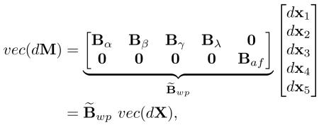with ${\tilde{\mathrm{B}}}_{wp}\in {\mathbb{R}}^{8T\times 6d}$ and 0 is a matrix of zeros.

Finally, from (5)-(7), the Jacobian terms of this camera model can be computed as

$${\mathrm{J}}_j=\left(\right[{\mathrm{s}}_j^{T}1]\otimes {\mathrm{P}}_j^{\perp }{\Pi }_j){\tilde{\mathrm{B}}}_{wp}.$$

Unlike in the previous sections, here the extended basis B̃_wp must be recomputed in each iteration to update the partial derivatives in B_α, B_β, B_γ, and B_λ. Thus, B̃_wp can be considered only as a local basis at the current location of the smooth parameter manifold.

The last step in each iteration shown in Algorithm 1, orthogonalization of M, is no longer necessary.

4 Non-Rigid SFM: Estimating a Smooth-Trajectory in Shape Space

In this section, we solve for non-rigid SFM by estimating the smooth time-trajectory of a 3D shape as represented by a point moving in a linear shape space. Without loss of generality, we assume W is complete and derive our 3D shape trajectory approach. Subsequently, we offer an algorithm for cases with missing data.

4.1 Solving for a shape trajectory

Let $\mathrm{W}\in {\mathbb{R}}^{2T\times n}$ as in (14) and consider the rank-r factorization method, with r = 3K + 1, proposed by Bregler et al. [5] for non-rigid scenes,

with $\mathrm{D}\in {\mathbb{R}}^{2T\times 3T}$, $\mathrm{C}\in {\mathbb{R}}^{T\times K}$, and $\mathrm{S}\in {\mathbb{R}}^{3K\times n}$. The predefined constant K is the number of 3D basis shapes ${\widehat{\mathrm{S}}}_k\in {\mathbb{R}}^{3\times n}$ defining a linear shape space in $\mathrm{S}={\left[{\widehat{\mathrm{S}}}_1^T{\widehat{\mathrm{S}}}_2^T\dots {\widehat{\mathrm{S}}}_K^T\right]}^T$.

The column space factor M is composed of a block-diagonal rotation matrix D,

$$\mathrm{D}=\left[\begin{array}{cccc}\hfill {\widehat{\mathrm{R}}}_1\hfill & \hfill \hfill & \hfill \hfill & \hfill \hfill \\ \hfill \hfill & \hfill {\widehat{\mathrm{R}}}_2\hfill & \hfill \hfill & \hfill \hfill \\ \hfill \hfill & \hfill \hfill & \hfill \ddots \hfill & \hfill \hfill \\ \hfill \hfill & \hfill \hfill & \hfill \hfill & \hfill {\widehat{\mathrm{R}}}_T\hfill \end{array}\right],$$

and a shape coordinate matrix C. Each row ${\mathrm{c}}_t^T\in {\mathbb{R}}^K$ of C has the coordinates of the 3D shape in the t^th image with respect to the shape basis in S. Here, we also consider ${\mathrm{c}}_t^T=c\left(t\right)$ as a single point in shape space that defines a single smooth 3D shape trajectory over time.

We assume that the smooth 2D trajectories in W reflect not only smooth camera motion, but also the smooth deformation of the observed 3D structure over time. This means that each shape coordinate $c_{tk}\in \mathbb{R}$ (k = 1, 2, … , K) is assumed to vary smoothly with t. Then, we represent C using K compact cosine series,

$$\mathrm{C}=\left[\begin{array}{ccc}\hfill c_{1,1}\hfill & \hfill \dots \hfill & \hfill c_{1,K}\hfill \\ \hfill ⋮\hfill & \hfill \ddots \hfill & \hfill ⋮\hfill \\ \hfill c_{T,1}\hfill & \hfill \cdots \hfill & \hfill c_{T,K}\hfill \end{array}\right]={\Omega }_d\left[{\mathrm{x}}_1,\dots ,{\mathrm{x}}_K\right],$$

with ${\mathrm{x}}_k\in {\mathbb{R}}^d(k=1,\dots ,K)$,

$$\mathrm{C}={\Omega }_d\mathrm{X},\mathrm{X}\in {\mathbb{R}}^{d\times K}.$$

Assuming W is complete, t is estimated simply as the mean column of W. Then, to recover Euclidean shapes and cameras, we consider S implicitly and solve for

$$\mathrm{M}=\mathrm{D}({\Omega }_d\mathrm{X}\otimes {\mathrm{I}}_3),$$ (18)

with D subject to camera orthonormality constraints, i.e., ${\widehat{\mathrm{R}}}_t{\widehat{\mathrm{R}}}_t^T={\mathrm{I}}_2$, ∀t. For now, let’s assume D has been computed by an initialization algorithm. We will define this algorithm below. Thus, we only need to solve for the rank-K shape trajectory X in the DCT domain.

For a fixed D, the factor C = Ω_dX is defined only up to a full-rank ambiguity $\mathrm{Q}\in {\mathbb{R}}^{K\times K}$; equivalently, M in (18) is defined only up to an ambiguity $\mathrm{Q}\otimes {\mathrm{I}}_3$. Therefore, as in Section 2.2, we can initialize X with a coarse solution X₀ = [I_K 0]^T, leading to

$${\mathrm{M}}_0=\mathrm{D}({\Omega }_d{\mathrm{X}}_0\otimes {\mathrm{I}}_3)=\mathrm{D}({\Omega }_K\otimes {\mathrm{I}}_3).$$ (19)

Note that K < d and the initial rank-3K solution in (19) can only use K low-frequency vectors in the DCT basis.

The 3D point trajectory approach (PTA) in [2] defines M = DΤ, where Τ has the same columns as (Ω_K ⊗ I₃) in (19), but in a different order. Therefore, our coarse initial solution M₀ is equivalent to the final solution M of PTA (with factor S presenting a different order of rows). Note that the PTA method cannot consider additional DCT basis vectors without increasing K, leading to a higher rank of M. Our 3D shape trajectory approach, on the other hand, can consider any number d = K, … , T of DCT basis vectors because the linear combination represented by X constrains M to be of rank-3K. That is, our method can better model structure deformation presenting higher-frequency components in the DCT domain, yielding better 3D shape reconstructions.

Empirically, we have found that the coarse solutions computed by PTA contain accurate estimates of the rotation matrices in D. We iteratively run PTA with increasing values of $K\in \{1,2,\dots ,[\frac{n}{3}\left]\right\}$, obtaining a solution denoted as D_K. Iterations stop automatically when there is no additional improvement in the average camera orthonormality,

$$\epsilon \left({\mathrm{D}}_K\right)=\frac{1}{T}\sum _{t=1}^T{\mid \mid {\mathrm{I}}_2-{\widehat{\mathrm{R}}}_t{\widehat{\mathrm{R}}}_t^T\mid \mid }_F^2.$$

Given D = D_K, we then solve for M as a function of X only. The first differential of M in (18) is given by

(20)

Next, consider vec(dX ⊗ I₃) = Vvec(dX), with $\mathrm{V}\in {\mathbb{R}}^{9dK\times dK}$ a binary mapping matrix. From (12) and (20), the Jacobian terms for the update step vec(dX) are

$${\mathrm{J}}_j=({\mathrm{s}}_j^T\otimes {\mathrm{P}}_j^{\perp }{\Pi }_j{\mathrm{B}}_{nr})\mathrm{V}.$$

with ${\mathrm{s}}_j={\mathrm{M}}_j^{†}({\mathrm{w}}_j-{\mathrm{t}}_j)$. For X with dimensions d × K, the constant and sparse matrix V is defined as [20],

$$\mathrm{V}={\mathrm{I}}_K\otimes \left[\right({\mathrm{K}}_{3d}\otimes {\mathrm{I}}_3\left)\right({\mathrm{I}}_d\otimes vec\left({\mathrm{I}}_3\right)\left)\right],$$

where the permutation matrix ${\mathrm{K}}_{3d}\in {\mathbb{R}}^{3d\times 3d}$ satisfies vec(A^T) = K_3dvec(A), for any $\mathrm{A}\in {\mathbb{R}}^{3\times d}$.

4.2 Non-Rigid SFM with missing data

The method above can estimate X using only the observed data in W. We now consider the initial estimation of t and D (the camera motion) in cases of missing data. To compute t and D from a coarse solution as above, we first recover a complete, rank-r W via the factorization

with a predefined r ∈ {4, 5, … , 3K + 1} and the DCT basis B_af of Section 3. Instead of considering the trajectory of an affine camera, here B_af is a basis for individual, smooth 2D point trajectories in the column space of W.

Note that a common solution for M corresponds to the eigenvector matrix U of WW^T (if W is complete). Here, our solution M = B_afX can be seen as using linear combinations of the DCT basis vectors to approximate the eigenvectors in U. Indeed, the DCT basis vectors have been found to be good approximations of the Karhunem-Loeve (eigenfunction) transform of first-order Markov processes [18]. Also, the Markov assumption is used in algorithms that track the 2D points in W [11].

5 Experimental Results

In this section we provide extensive experimental validation for the proposed algorithms. General matrix factorization performance is first assessed on different, synthetic and real datasets. Subsequently, we apply our methods on rigid and non-rigid SFM data.

5.1 Fitting low-rank matrices

Our initial experiments analyze the general performance of our CSF method in its simplest form (i.e., with a canonical basis I and without a mean column vector t) in the low-rank factorization of synthetic and real data matrices with missing data. The method is evaluated against the LM-S algorithm [8] and its Gauss-Newton variant, LM-S_GN (presented in the supplementary file). We also provide results using PowerFactorization (PF) [16] as a baseline algorithm.

We start by generating a random 20 × 30 matrix W of rank 3 with values uniformly distributed in the interval [0; 1]. Then, we add Gaussian noise with standard deviation σ_n and randomly occlude ρ% of the matrix entries. The algorithms above are used to compute a rank-3 factorization W = MS starting from the same initial factor M = M₀, which is generated randomly and then refined with 20 iterations of the PF method. We always set the initial damping scalar to δ₀ = 10⁻⁴. Each algorithm runs until the change in the cost value (2) is less than 10⁻¹⁰ or until the number of iterations reaches 1,000. Note that, although we know the ground truth data, we do not know where the optimal solution for the matrix with missing data is [8]. Therefore, we first run all algorithms and, considering the solution obtained by each algorithm, we then define the trial’s target (i.e., “optimal”) cost as the smallest cost observed.

We perform 500 trials, with σ_n and ρ fixed, and report the frequency (%) with which a method failed to match the trial’s “optimal cost”. We consider two cost values as equivalent if their absolute difference is below 10⁻⁷. Results for different values of σ_n and ρ are shown in Table 1, which also includes the average number of iterations performed by each method. As expected, the simple PF method converges very slowly and is competitive only when ρ is very small. For ρ ∈ {25%, 50%}, CSF’s performance is either comparable or better than that of LM-S and LM-S_GN. CSF also converges faster than LM-S_GN for smaller fractions of missing data. With ρ = 75%, CSF clearly outperforms the other methods. These results are highly revelant to SFM, where the number of missing entries is usually large (> 75%).

TABLE 1.

Algorithm performances on random matrices with missing data: frequency of sub-optimal solutions (%) and average number of iterations (in parenthesis).

ρ(%), σn	PF	LM-S	LM-SGN	CSF
25, .1	23 (313)	1 (16)	4 (82)	3 (57)
25, .2	30 (391)	3 (17)	6 (93)	3 (65)
25, .4	28 (381)	3 (16)	8 (108)	5 (74)
50, .1	71 (813)	12 (51)	14 (96)	11 (79)
50, .2	76 (831)	15 (58)	14 (105)	12 (89)
50, .4	77 (869)	18 (61)	19 (120)	16 (103)
75, .1	100 (1000)	69 (356)	62 (380)	42 (549)
75, .2	100 (1000)	72 (376)	54 (419)	46 (586)
75, .4	100 (1000)	77 (421)	65 (473)	44 (698)

A second, similar experiment considers the three real datasets used in [6] and [8]: (i) the dinosaur on a turn table, with rank-4 $\mathrm{W}\in {\mathbb{R}}^{72\times 319}$ and 76.9% missing data; (ii) the occluded motion of a giraffe, with rank-6 $\mathrm{W}\in {\mathbb{R}}^{240\times 166}$ and 30.2% missing data; and (iii) the face illumination data under a moving light source, with rank-4 $\mathrm{W}\in {\mathbb{R}}^{20\times 2944}$ and 41:7% missing data. For each dataset, the smallest known root-mean-square error (RMSE) of the observed entries, as previously published [6], gives the target value that indicates optimal convergence.

We performed 100 trials corresponding to 100 different initial factors M generated as above. Each algorithm was allowed to run for at most 500 iterations. Table 2 shows the frequency of sub-optimal convergence (%) and average number of iterations for each algorithm. We first note that on the face dataset, all algorithms except PF often converged to a sub-optimal solution whose cost is only .45% (about 10⁻⁴) higher than that of the optimal solution. If this solution is considered equivalent to the optimal one, the new sub-optimal convergence frequencies are 9% (LM-S), 8% (LM-S_GN), and 1% (CSF). Nevertheless, in the results above, CSF either provides better solutions or computes equivalent solutions with fewer iterations as compared to the other methods.

TABLE 2.

Algorithm performances on real datasets with missing data: frequency of sub-optimal convergence (%) and average number of iterations (in parenthesis).

Dataset	PF	LM-S	LM-SGN	CSF	CSF-Baf
Dinosaur	100 (500)	26 (225)	3 (92)	1 (101)	0 (12)
Giraffe	100 (500)	0 (192)	0 (86)	0 (61)	0 (49)
Face	100 (500)	65 (36)	62 (64)	62 (43)	–

Because the columns of the dinosaur and giraffe matrices have measurements (alternated x- and y-coordinates) that vary smoothly over subsequent pairs of rows, we also computed factorizations with the CSF-B_af variant of our method. We used the full B_af basis and started with the deterministic initialization in (13) as a coarse initial solution. CSF-B_af presented optimal convergence on both datasets, without the initial use of PF.

5.2 Computing rigid SFM

Our first experiment on rigid SFM considers a synthetic sphere dataset with known 3D points (n = 100), located on its surface, and also known camera matrices (T = 90) describing a smooth trajectory over time, Fig. 3. The real occlusion pattern for the simple spherical shape can be easily determined and the resulting observation matrix $\mathrm{W}\in {\mathbb{R}}^{180\times 100}$ is missing 50% of its entries.

Fig. 3.

Smooth camera trajectory in the synthetic sphere dataset.

Results of our SFM methods with affine (CSF-B_af) and weak-perspective (CSF-B_wp) cameras are compared against those of PF, LM-S, LM-S_GN, and the Wiberg algorithm [31]. Euclidean upgrade is applied to the results of affine methods. All results are aligned (rotated and scaled) with the ground-truth shape and motion before comparison. On the noiseless W, the methods above provide camera and shape reconstructions with nearly zero error. Our CSF methods are run with only 30% of the DCT basis vectors (d = .3T).

In our experiment, we analyze how the performance of these methods degrades with different levels of Gaussian noise added to W. We now set ${\sigma }_n={\widehat{\sigma }}_n\sigma \left(\mathrm{W}\right)$, where ${\widehat{\sigma }}_n\in [.05,.25]$ and σ(W) indicates the scale of the entries of W. For any matrix A with m rows, let

$$\sigma \left(\mathrm{A}\right)=\frac{1}{m}\sum _{r=1}^m{\sigma }_r,$$ (21)

where σ_r is the standard deviation of the available entries in the r^th row of A. For each value of ${\widehat{\sigma }}_n$, we perform 100 trials and report the average error of the recovered 3D shape (e_S) and camera rotations (e_R). The error e_S is the average Euclidean distance between original and recovered 3D points, normalized by the radius of the original 3D sphere. Let the original and estimated rotations be ${\widehat{\mathrm{R}}}_t^{\ast }$ and ${\widehat{\mathrm{R}}}_t$, then e_R is

$$e_R=\frac{1}{T}\sum _{t=1}^T{\mid \mid {\widehat{\mathrm{R}}}_t^{\ast }-{\widehat{\mathrm{R}}}_t\mid \mid }_F.$$ (22)

CSF-B_af and CSF-B_wp were run with deterministic initializations. The other methods require random initializations and often provided very poor solutions in our experiments. For this reason, in each trial they were run with five different random initializations; the result with the smallest RMSE for the reconstructed W was chosen.

The average errors in Table 3 show that the shape estimates of all methods seem to be similarly affected by noise up to ${\widehat{\sigma }}_n=.125$. Also, a significant difference is seen for the camera estimates with ${\widehat{\sigma }}_n>.05$. Affine methods overfit noise in the data due to the extra degrees of freedom in their camera model. CSF-B_af and CSF-B_wp attenuate this problem by enforcing smoothness on the camera trajectory. CSF-B_wp outperforms all methods by further constraining the camera axes to be orthogonal and of equal length. This result is of special importance to SFM applications that rely more on the motion factor.

TABLE 3.

Results of rigid SFM methods on the sphere dataset.

Method	${\widehat{\sigma }}_n=.05$		${\widehat{\sigma }}_n=.125$		${\widehat{\sigma }}_n=.25$
	eS	eR	eS	eR	eS	eR
PF	.0163	.0250	.0818	.1247	.2092	.2839
LM-S	.0169	.0255	.0845	.1284	.1780	.2690
LM-SGN	.0170	.0255	.0845	.1284	.1777	.2686
Wiberg	.0163	.0250	.0806	.1242	.1695	.2569
CSF-Baf	.0163	.0151	.0806	.0731	.1651	.1513
CSF-Baf	.0156	.0130	.0779	.0606	.1586	.1280

The average runtimes in seconds (per initialization, on a single-core 2.6 GHz processor) were: .2 (PF), 18.2 (LM-S), 14.9 (LM-S_GN), 128.5 (Wiberg), 1.1 (CSF-B_af), and 8.0 (CSF-B_wp). The simple PF is fast but often provides poor estimates, even with a maximum of 10,000 iterations (versus 500 for the other methods). CSF-B_af and CSF-B_wp are also very fast. Typically, CSF-B_wp performs more iterations than CSF-B_af – for better convergence on long sequences (large T), we run CSF-B_wp in a coarse-to-fine manner, increasing d ∈ {.1T, .2T, .3T}. We also note that the Wiberg method does not scale well for application on large matrices due to the size of the system of equations it has to solve in each iteration.

Our experiments also considered the complete dinosaur dataset with 4,983 tracks (of which 2,300 are defined on only two images).¹ The dinosaur sequence is arguably the most popular dataset used to evaluate rigid SFM algorithms, with results published on different subsets of its 2D point tracks. For comparison against previously published results, we consider a subset of 2,683 tracks (points tracked in at least 3 images) and the subset of 319 tracks described above.

Results of the methods above are also compared to those of the following algorithms: Damped-Newton (DN) [6], the Deviation Parameter (DP) for subspace constraints [19], Minimal Missing Elements (MME) [7], Camera Basis (subspace) Constraints (CBC) [28], and the Euclidean PowerFactorization (EPF) method in [21]. Finally, we also compare the result of CSF-B_wp to that obtained with projective SFM followed by Euclidean bundle adjustment (ProjSFM-BA) [22]. Because the groundtruth 3D shape and cameras are not available, we compare RMSE values for the reconstructed W and also the mean/maximum 2D reprojection errors (in pixels) of the best solutions provided by each method. For this numerical comparison on the relatively short dinosaur sequence (T = 36), our CSF methods were both initialized (deterministically) with full DCT bases.

In Table 4, each incomplete row contains only the results reported in the original publication due to the algorithm not being available in our experiments. Because these algorithms use factorization models with different numbers of degrees of freedom, we define three main groups of methods. In this case, models with more degrees of freedom are expected to be associated with lower RMSE and 2D error values. However, we note that CSF-B_wp yielded lower 2D reprojection errors compared to the affine SFM methods. In the dinosaur dataset, the performance of CSF-B_wp is very close to that of the projective SFM method with bundle adjustment, despite the non-negligible perspective distortion in the data. Fig. 4(b)-(c) show the 3D shape recovered by CSF-B_wp.

TABLE 4.

Results of rigid SFM methods on different subsets of the dinosaur dataset.

Method (model)	319 point tracks (76.9% missing)		2,683 point tracks (87.8% missing)		4,983 point tracks (90.8% missing)
	RMSE	mean/max 2D error	RMSE	mean/max 2D error	RMSE	mean/max 2D error
CSF-Baf (1)	1.0847	.6286 / 38.8381	1.3370	.7129 / 39.9999	1.1346	.5133 / 39.9999
LM-S, LM-SGN (1)	1.0847	.6287 / 38.8376	1.3370	.7131 / 39.9999	1.1346	.5135 / 39.9997
DN (1)	1.0847	–	–	–	–	–
DP (1)	1.5482	1.0131 / 39.4277	2.0201	1.9103 / 40.2124	1.7142	1.6233 / 40.1713
MME (1)	–	–	–	2.4017 / 72.4467	–	1.8438 / 72.4467
CSF-Baf (2)	1.2702	.8810 / 41.4078	1.4294	.8610 / 42.5002	1.2176	.6808 / 42.4961
Wiberg (2)	1.2702	.8810 / 41.4081	1.4294	.8609 / 42.5002	1.2176	.6808 / 42.4959
DN (1*)	1.2702	–	–	–	–	–
CBC (2)	1.8120	.9730 / 76.4071	2.9126	.8884 / 92.7365	2.4538	.7044 / 92.7399
PF (2)	1.4139	1.0091 / 41.1094	2.0604	1.2238 / 64.1713	2.4531	1.5846 / 61.3726
CSF-Bwp (3)	1.3031	.8757 / 43.8770	1.4833	.8122 / 44.6721	1.2641	.6472 / 44.7587
EPF 3)	1.3705	– / 21	–	–	–	–
ProjSFM-BA (3*)	–	–	–	–	–	.64 / 41.5

^†Models: (1) general rank-4 factors (no mean column); (2) affine SFM; (3) Euclidean (weak-perspective) SFM; (3*) projective SFM with Euclidean bundle adjustment; (1*) penalty terms imposed on model (1) to favor orthogonality of camera axes. Error values are given in pixels.

Fig. 4.

Results on the 4,983 point set (90.8% missing) of the dinosaur dataset: (a) one of the 36 images of the sequence; (b)-(c) side and frontal views of the Euclidean 3D shape recovered by CSF-B_wp; and 2D point tracks reconstructed by CSF-B_wp (d) and by the best affine methods (e).

Information on the ground-truth motion is actually available because we know the dinosaur is on a turn-table. Thus, the reconstructed W must describe 2D point trajectories that are all concentric ellipses. Indeed, the result of CSF-B_wp indicates correct motion recovery, Fig. 4(d). The best affine methods in our comparison (CSF-B_af , LM-S, LM-S_GN, and Wiberg) overfit noise and outliers and recover an incorrect motion pattern, Fig. 4(e). This problem is inherent in all affine SFM methods (incorrect 2D trajectories are also shown in [6], [8]). Also note this fact is independent of the Euclidean upgrade step, which does not affect reprojection.

The robust CBC method uses random sampling to tolerate outliers when computing subspace constraints and triangulating 3D points. Thus, CBC yields higher RMSEs as compared to the other methods. Table 4 shows that 2D reprojection error decreases as more point tracks are available for outlier/inlier identification – we computed camera constrains from triplets of frames presenting at least 15 tracks in common. In [28], CBC was found to provide the best solutions among the main subspace constraint methods. Here, error values are higher than those in [28] because we did not remove outliers before the comparison against non-robust methods. We note that our CSF methods do not explicitly address the problem of outliers and may fail if the input data present gross measurement errors. Future work will investigate the use of robust error terms [9], [12] in our cost functions.

In another experiment, we applied the Kanade-Lucas-Tomasi (KLT) feature tracker [27] on a 200-image teddy bear sequence [28]. We selected 806 point tracks appearing in at least 10 images. Due to occlusion, the resulting matrix $\mathrm{W}\in {\mathbb{R}}^{400\times 806}$ is missing 88.6% of its entries. For numerical comparison, both CSF methods considered a full DCT basis. CSF-B_wp adopted a coarse-to-fine strategy with d ∈ {.1T, .2T, .3T, … , T} increased each time convergence to a coarser solution was detected. Table 5 gives the 2D errors obtained with the algorithms described above on our teddy bear dataset. CSF-B_af provides equivalent or better solutions as compared to the other methods. Also, CSF-B_wp directly reconstructs the Euclidean 3D shape with only a slight increase in 2D error – its camera model captures less of the noise in the data. Fig. 5 shows the 3D shape reconstructed with CSF-B_wp. On this long sequence (T = 200) with smooth motion, the difference in the results of CSF-B_wp with a full DCT basis (d = T) and with d = .3T is very small, e_R = .0175 and e_S = .0229 (here e_S is normalized by σ(S) as in (21)). With d = .3T, the runtime of CSF-B_wp drops from 27.3 to 3.6 minutes (4 to .7 minute for CSF-B_af). Wiberg took on average 4.2 hours.

TABLE 5.

Results of rigid SFM methods on the teddy bear dataset.

Method (model)	RMSE	mean/max 2D error
CSF-Baf (1)	.4925	.4527 / 7.4998
LM-S, LM-SGN (1)	.4925	.4527 / 7.4998
DP (1)	.5911	.4977 / 13.8324
CSF-Baf (2)	.6174	.5689 / 10.7385
Wiberg (2)	.6174	.5689 / 10.7385
CBC (2)	.7487	.6478 / 14.1339
PF (2)	1.2125	.8649 / 27.5116
CSF-Bwp (3)	.6310	.5792 / 10.6524

^†Models are as in Table 4. Error values are given in pixels.

Fig. 5.

Result of CSF-B_wp on 806 point tracks (88.6% missing) of the teddy bear sequence: (a) image in the sequence; (b) input 2D tracks; (c)-(d) frontal and top views of the recovered Euclidean 3D shape.

5.3 Computing non-rigid SFM

First, we evaluate our non-rigid SFM algorithm on complete datasets with known 3D shapes for each frame, also simulating missing data and noise. Then, we present results on real datasets with and without occlusion. The number of frames (T) and the number of point tracks (n) are indicated as (T/n) after a dataset’s name.

We start with the motion capture sequences: drink (1102/41), pick-up (357/41), yoga (307/41), stretch (370/41), and dance (264/75) used in [2]; face1 (74/37) of [24]; face2 (316/40) and walking (260/55) of [30]. We also use the synthetic bending shark (240/91) of [30]. Note that a different shark dataset appears in [2]. We use only the original one in [30].

To allow for comparison against the results reported in [2], we used the same procedure and error metrics therein. For each dataset, the complete 2D point trajectories in W are obtained by applying an orthographic projection on the sequence of 3D shapes. Because the solution of non-rigid SFM methods is defined up to an arbitrary 3 × 3 rotation, we compute a single rotation that best aligns all reconstructed and original 3D shapes. Let e_tj be the reconstruction error (i.e., Euclidean distance) for the j_th 3D point of frame t. We then compute a normalized mean 3D error over all points and frames,

$$e_{3D}=\frac{1}{{\sigma }_{e}Tn}\sum _{t=1}^T\sum _{j=1}^n{e}_{tj},{\sigma }_e=\frac{1}{T}\sum _{t=1}^T\sigma \left({\mathrm{S}}_t\right),$$

with σ(·) as in (21) and ${\mathrm{S}}_t\in {\mathbb{R}}^{3\times n}$ the original 3D shape in frame t. The first four motion capture sequences have artificial rotations applied on them. We thus compare original and estimated rotations using e_R as in (22).

Table 6 compares the performance of our 3D shape trajectory approach, CSF-B_nr, against four state-of-the-art, non-rigid SFM methods: (i) the shape basis constraints (XCK) method² [32]; (ii) the algorithm modeling 3D shape using probabilistic principal component analysis (EM-PPCA) [30]; (iii) the Metric Projections (MP) method³ [24]; and (iv) the DCT-based 3D point trajectory approach (PTA) [2].

TABLE 6.

Performance of non-rigid SFM methods on synthetic and motion capture data. For the related PTA and CSF-B_nr methods, factorization rank is also indicated by the value of K in parenthesis.

Dataset	XCK		EM-PPCA		MP		PTA		CSF-Bnr
	eR	e 3D	eR	e 3D	eR	e 3D	eR	e3D (K)	eR	e3D (K)	initial e3D (K)
Drink	.3359	3.5186	.2906	.3393	.2859	.4604	.0058	.0250 (13)	.0055	.0223 (6)	.0854 (6)
Pick-up	.4687	3.3721	.4277	.5822	.2506	.4332	.1549	.2369 (12)	.1546	.2301 (6)	.2685 (6)
Yoga	1.2014	7.4935	.8089	.8097	.8711	.8039	.1059	.1625 (11)	.1021	.1467 (7)	.1528 (7)
Stretch	.9489	4.2415	.7594	1.1111	.8174	.8549	.0549	.1088 (12)	.0489	.0710 (8)	.0966 (8)
Dance	–	2.9962	–	.9839	–	.2639	–	.2958 (5)	–	.2705 (2)	.3259 (2)
Face1	–	–	–	.0434	–	.0734	–	.1247 (3)	–	.0637 (5)	.1487 (3)
Face2	–	–	–	.0329	–	.0357	–	.0444 (5)	–	.0363 (3)	.0451 (3)
Shark	–	–	–	.0501	–	.1571	–	.1796 (9)	–	.0081 (3)	.3195 (3)
Walking	–	–	–	.4917	–	.5607	–	.3954 (2)	–	.1863 (2)	.6823 (2)

Following the methodology in [2], we ran the algorithms with different values of K ∈ {2, 3, … , 13}, reporting the best result. Table 6 also shows the value of K for the best solutions obtained with PTA and CSF-B_nr for comparison. We also report the initial error of CSF-B_nr because it shows the error that PTA would provide with the same K and rotations in D. In all runs, CSF-B_nr had the number of DCT basis set to d = .1T, except for the two face datasets on which we set $d=\frac{T}{3}$ due to the presence of higher frequency deformations.

Our results, as shown in Table 6, are consistently similar or better than the best results provided by the other methods on each dataset. As compared to PTA, CSF-B_nr computes better solutions and at a lower rank r = 3K + 1 by more efficiently using higher DCT frequency components. Furthermore, our simple strategy of iterating over K while computing factor D also provides better Euclidean camera estimates than plain PTA.

EM-PPCA, MP, and CSF-B_nr provide comparable results on the face2 dataset, which has mostly rigid motion with high-frequency deformation seen on the lower-lips and chin. In this case, CSF-B_nr requires at least 75% of all DCT components (d = .75T) to provide a mean 3D error (.0328) that is smaller than that of EM-PPCA. PTA is not capable of modeling this high-frequency deformation and recovers a mostly rigid mouth, Fig. 6. On the much shorter face1 sequence, CSF-B_nr obtains an error improvement of only .0012 with a larger d. Setting d > .1T resulted in no significant improvement to the CSF-B_nr solutions on the other datasets.

Fig. 6.

Overlay of 316 unrotated 3D shapes in the face2 sequence. Deformation is seen predominantly on the lower-lips and chin. CSF-B_nr can capture this high-frequency deformation better than PTA.

CSF-B_nr is the only method that can accurately reconstruct the deformation of the bending shark. Furthermore, with a full DCT basis, the resulting e_3D is negligible (.00004) and perfect reconstruction is achieved. Fig. 7 shows the three best shark reconstructions of Table 6. XCK fails on this dataset due to the bending shark presenting a 2D (degenerate) deformation mode [30].

Fig. 7.

Results on the bending shark sequence. Reconstructed 3D shapes (blue circles) are shown against the original 3D data (dark dots). Frames 20, 50, 80, 115, 148, 175, and 200 are displayed above.

The motion capture sequences containing highly articulated bodies also show the superiority of CSF-B_nr and PTA compared to XCK, EM-PPCA, and MP. On the smoothly deforming shapes in the drink, pick-up, and yoga sequences (used in [2]), the improvement offered by CSF-B_nr over PTA is marginal. On the other hand, the results on the more difficult walking sequence of [30] (Fig. 8) highlight the advantages of using our 3D shape trajectory approach (no artificial rotation was added to this sequence). MP provides comparable results with CSF-B_nr on the dance sequence. The supplementary file includes additional examples.

Fig. 8.

Results on the walking sequence. Reconstructed 3D shapes (blue circles) are shown against the original 3D data (dark dots). Frames 34, 74, 122, 160, 198, 223, and 255 are displayed above.

To simulate missing data in the shark and walking datasets, we randomly discard ρ% of the 2D entries in W. Before applying CSF-B_nr (with K as in Table 6), we compute D and t by first using CSF-B_af to reconstruct the complete 2D point trajectories in W. CSF-B_af was run with d = .25T and rank r = 7. Let W₀ be the complete matrix, we normalize the 2D reconstruction error for the incomplete W by σ(W₀) as in (21).

On the smooth shark deformation, results are visually similar to those in Fig. 7 with ρ up to 95% (see images in the supplementary file). Of 10 runs with ρ = 95%, the average (maximum) 2D reconstruction error for W was .0015 (.0029). The average (maximum) 3D error after running CSF-B_nr was .0163 (.0488). On the walking sequence, results with ρ = 75% are still visually similar to those in Fig. 8. After 10 runs, the average (maximum) 2D and 3D errors were .0508 (.0548) and .2063 (.3910), respectively. These results on incomplete data are still better than those of XCK, EM-PPCA, MP, and PTA on the complete shark and walking datasets.

On the complete face2 dataset, the performances of EM-PPCA, MP, PTA, and CSF-B_nr are more similar than on the other sequences. We thus analyzed their average e_3D with different levels of random occlusion and noise (simulated independently) on W of face2. EM-PPCA and MP handle cases of missing data by adopting an alternation approach as in PowerFactorization. PTA does not handle occlusions and was tested with added noise only. All methods were run with their best parameter K for the complete data (K = 5 for EM-PPCA, MP, PTA; K = 3 for CSF-B_nr). After random occlusion, we ensured that W had at least 3K_max+1 entries (K_max = 5) in each row and column. On the high-frequency deformation and motion of face2 (combined in the columns of W), the initial CSF-B_af step of CSF-B_nr reconstructed the 2D point trajectories in W with d = .5T and r = 5. Results were averaged over 100 trials and are shown in Fig. 9.

Fig. 9.

Reconstruction errors on the face2 sequence with missing data and noise simulated independently (averages over 100 trials).

In our trials on face2 with missing data, EM-PPCA was unstable and presented both small and very large errors for random occlusions ρ as low as 10%. Thus, Fig. 9(a) shows the results of CSF-B_nr in comparison to those of MP, which was shown in [24] to outperform EM-PPCA in a similar experiment on face2. Note that the average e_3D of MP begins to increase with ρ above 30%, while that of CSF-B_nr presents almost no variation over all the tested levels of random occlusion.

For levels of added Gaussian noise below .15σ(W) (15%), the increase in e_3D is similar for all four methods, Fig. 9(b). At 15% and above, small differences in performance are observed but the reconstructions still degrade only gradually with the level of noise. Because PTA largely oversmoothes the deformation of face2, its performance suffers a smaller penalty as compared to that of the other methods. At high noise levels, correct 3D shape reconstruction seems to require additional information on the nature of the 3D shapes and noise [12].

The average runtimes of the algorithms on the face2 trials at 5% noise level were, in minutes: 2.52 (EMPPCA), .34 (MP), .05 (PTA), and .40 (CSF-B_nr, of which .15 was spent to compute D). These times were similar to those observed for the algorithms on the original data. PTA is fast due to its use of SVD. Runtimes in minutes on face2 trials with 30% missing data were: 2.85 (EMPPCA), 3.66 (MP), and 2.29 (CSF-B_nr). This runtime of CSF-B_nr includes time spent running CSF-B_af (.82) and computing D (.19). At above 20% random occlusion, CSF-B_nr was faster than MP and EM-PPCA.

We also applied CSF-B_nr to the (complete) real dataset cubes (200/14) of [2]. With K = 2 and d = .1T, the solution of CSF-B_nr has mean (maximum) 2D reprojection error of .4958 (2.0672) pixel. The solution of PTA has an error of 1.6589 (4.8602) also with K = 2. Images and additional results are given in the supplementary file.

Finally, an application of our non-rigid SFM method is in the interpretation of the facial expression component of sign languages from video [10]. In this case, head rotation and hand gesticulation often cause the occlusion of facial features, leading to incomplete 2D point tracks. We now consider a 115-image (4 seconds long) face close-up sequence of an American Sign Language (ASL) sentence. Facial landmarks were manually annotated in each image when visible. The resulting matrix $\mathrm{W}\in {\mathbb{R}}^{230\times 77}$ is missing 17.4% of its data and has small magnitude noise due to annotation errors caused by partial occlusion of facial features and motion blur in the video images. Fig. 10 shows six example images and their respective 3D face shapes recovered using CSF-B_nr (K = 2 and d = .5T, with the initial CSF-B_af step run as for face2 above). Figures with the results of EM-PPCA and MP are given in the supplementary file. For all tested values of K ∈ {2, 3, … , 13}, the result obtained with EM-PPCA presented visibly large 3D reconstruction errors for a number of facial points that are occluded frequently in each sequence (e.g., the lateral contours of the nose and the face). The results of CSF-B_nr and MP are visually similar and indicate correct recovery of pose and non-rigid 3D shape despite the occurrence of occlusion.

Fig. 10.

Results of CSF-B_nr on the ASL sequence (77 points, 17.4% missing data): (top) six out of 115 images with annotated facial landmarks in green; (middle,bottom) two orthogonal views of the recovered 3D shapes.

6 Conclusion

In this paper, we have addressed the classical computer vision problems of rigid and non-rigid SFM with occlusion. We started by assuming that the columns of the input data matrix W describe smooth 2D point trajectories over time. This assumption is equivalent to considering that 2D observations in W are obtained by a single camera moving smoothly around a rigid structure. In non-rigid SFM, our assumption also requires the structure to deform only smoothly over time.

Our main contributions are two-fold: (i) we provide new models for the smooth time-trajectories of camera and deformable shape with a compact parameterization in the DCT domain; and (ii) we derive a family of efficient Column Space Fitting (CSF) methods to estimate such trajectories while tolerating cases in which W is presented with missing data.

In rigid SFM, we consider a weak-perspective camera model from the outset and directly reconstruct Euclidean 3D shape without requiring post-processing steps. Our results on synthetic and real SFM datasets with noise and high percentages of missing data were positively compared to the state of the art.

In non-rigid SFM, we propose a novel 3D shape trajectory approach that solves for the deformable structure as the trajectory of a single point in an implicitly defined linear shape space. A comparison against state-of-the-art algorithms show that our method can better model complex articulated deformation with higher frequency DCT components while still maintaining the low-rank factorization constraint. We also demonstrate that our non-rigid SFM algorithm can tolerate high percentages on missing data in the input matrix W with only a small penalty in 3D reconstruction accuracy.

Future work will investigate the integration of our weak-perspective camera model into our non-rigid SFM approach. We will also consider the automatic selection of the number of elements in the DCT and shape bases using regularization terms that balance the tradeoff between higher model complexity (r, K, and d) and smaller fitting error [23], [25], [30]. Our CSF algorithms may also benefit from a robust error term in order to better tolerate the presence of outliers in W. Finally, non-linear models for the column space of W shall be considered.

Appendix A

Derivation of the Jacobian Terms in CSF

Consider vec(u^T v) = vec(u)^Tvec(v), and vec(BXA) = (A^T ⊗ B)vec(X), for any column vectors u and v, and any matrices B, X, and A. The operator ⊗ is the Kronecker product. Also, let the matrix ${\mathrm{K}}_{mr}\in {\mathbb{R}}^{mr\times mr}$ be a permutation satisfying vec(M^T) = K_mrvec(M).

By following a Gauss-Newton approach, the first and second differentials of f in (4) are

$$\begin{array}{cc}\hfill df& =\frac{1}{2}\sum _j(d{\mathrm{r}}_j^T{\mathrm{r}}_j+{\mathrm{r}}_j^{T}d{\mathrm{r}}_j)=\sum _j{\mathrm{r}}_j^{T}d{\mathrm{r}}_j,\hfill \\ \hfill d^{2}f& \approx \sum _{j}d{\mathrm{r}}_j^{T}d{\mathrm{r}}_j,\hfill \end{array}$$

with second order terms d²r_j neglected in d²f and

$$d{\mathrm{r}}_j=-d\left({\mathrm{M}}_j{\mathrm{M}}_j^{†}\right){\mathrm{w}}_j.$$ (23)

From [20], we have

$$d\left({\mathrm{M}}_j{\mathrm{M}}_j^{†}\right)={\mathrm{P}}_j^{\perp }d{\mathrm{M}}_j{\mathrm{M}}_j^{†}+{\left({\mathrm{P}}_j^{\perp }d{\mathrm{M}}_j{\mathrm{M}}_j^{†}\right)}^T.$$ (24)

with ${\mathrm{P}}_j^{\perp }$ as in (3). Considering M_j = Π_jM and expressing (23) as dr_j = −J_jvec(dM), the Jacobian terms are identified as

$${\mathrm{J}}_j={\mathrm{s}}_j^T\otimes {\mathrm{P}}_j^{\perp }{\Pi }_j+{\left({\Pi }_j^T{\mathrm{r}}_j\otimes {\mathrm{M}}_j^{†}\right)}^T{\mathrm{K}}_{mr}.$$ (25)

We now depart from the Gauss-Newton solution (25). First, notice that the right-most term in (24) vanishes when multiplied by ${\mathrm{r}}_j^T={\left(\right({\mathrm{P}}_j^{\perp }{\mathrm{w}}_j)}^T$ on the left,

$${\mathrm{r}}_j^T{\left({\mathrm{P}}_j^{\perp }d{\mathrm{M}}_j{\mathrm{M}}_j^{†}\right)}^T={\left({\mathrm{P}}_j^{\perp }d{\mathrm{M}}_j\left({\mathrm{M}}_j^{†}{\mathrm{P}}_j^{\perp }\right){\mathrm{w}}_j\right)}^T=0,$$

because the property My ${\mathrm{M}}_j^{†}={\mathrm{M}}_j^{†}{\mathrm{M}}_j{\mathrm{M}}_j^{†}$ implies

$${\mathrm{M}}_j^{†}{\mathrm{P}}_j^{\perp }={\mathrm{M}}_j^{†}\left(\mathrm{I}-{\mathrm{M}}_j{\mathrm{M}}_j^{†}\right)=0.$$

Thus, a Jacobian term (7) in CSF neglects the right-most term in (24) and (25). While there is no difference in the gradient vector, it can be shown that the Hessian matrix in (8) neglects terms of the form ${\Pi }_j^T{\mathrm{r}}_j{\mathrm{r}}_j^T{\Pi }_j\otimes {\mathrm{M}}_j^{†}{{\mathrm{M}}_j^{†}}^T$.

Our Hessian approximation, combined with the damping parameter δ in Algorithm 1, is efficient in providing adequate solution updates, vec(dM), despite the simpler form. CSF’s performance is positively compared to that of LM-S in Section 5. We also consider a Gauss-Newton derivation of LM-S (see the supplementary file).

For the rank-r factorization with a mean column t, we define ${\mathrm{s}}_j={\mathrm{M}}_j^{†}({\mathrm{w}}_j-{\mathrm{t}}_j)\in {\mathbb{R}}^{r-1}$. Then, the differential of the residual terms in (10) is

$$\begin{array}{cc}\hfill d{\mathrm{r}}_j& =d{\mathrm{P}}_j^{\perp }({\mathrm{w}}_j-{\mathrm{t}}_j)-{\mathrm{P}}_j^{\perp }d{\mathrm{t}}_j\hfill \\ \hfill & \approx -{\mathrm{P}}_j^{\perp }{\Pi }_{j}d{\mathrm{Ms}}_j-{\mathrm{P}}_j^{\perp }{\Pi }_{j}d\mathrm{t}\hfill \\ \hfill & \approx -{\mathrm{P}}_j^{\perp }{\Pi }_j\left[d\mathrm{M}d\mathrm{t}\right]\left[\begin{array}{c}\hfill {\mathrm{s}}_j\hfill \\ \hfill 1\hfill \end{array}\right]\hfill \\ \hfill & \approx -({\tilde{\mathrm{s}}}_j\otimes {\mathrm{P}}_j^{\perp }{\Pi }_j)vec\left(d\tilde{\mathrm{M}}\right),\hfill \end{array}$$

revealing the form of the Jacobian in (11). It is similar to (7) but has the extended terme s̃_j instead of s_j.

References

- [1].Akhter I, Sheikh Y, Khan S. In defense of orthonormality constraints for nonrigid structure from motion; Proc. IEEE Conf. Computer Vision and Pattern Recognition; 2009.pp. 1534–1541. [Google Scholar]
- [2].Akhter I, Sheikh YA, Khan S, Kanade T. Neural Information Processing Systems. Dec, 2008. Nonrigid structure from motion in trajectory space. [Google Scholar]
- [3].Bartoli A, Gay-Bellile V, Castellani U, Peyras J, Olsen S, Sayd P. Coarse-to-fine low-rank structure-from-motion; IEEE Conference on Computer Vision and Pattern Recognition; 2008.pp. 1–8. [Google Scholar]
- [4].Bertsekas D. Nonlinear Programming. Athena Scientific Press; 1999. [Google Scholar]
- [5].Bregler C, Hertzmann A, Biermann H. Recovering non-rigid 3d shape from image streams; Proc. IEEE Conference on Computer Vision and Pattern Recognition; 2000.pp. 690–696. [Google Scholar]
- [6].Buchanan AM, Fitzgibbon AW. Damped newton algorithms for matrix factorization with missing data; Proc. IEEE Conf. Computer Vision and Pattern Recognition; 2005.pp. 316–322. [Google Scholar]
- [7].Chen P, Suter D. Recovering the missing components in a large noisy low-rank matrix: Application to sfm. IEEE Trans. on Pattern Analysis and Machine Intelligence. 2004;26(8):1051–1063. doi: 10.1109/TPAMI.2004.52. [DOI] [PubMed] [Google Scholar]
- [8].Chen P. Optimization algorithms on subspaces: Revisiting missing data problem in low-rank matrix. International Journal on Computer Vision. 2008;80(1):125–142. [Google Scholar]
- [9].de la Torre F, Black M. Robust principal component analysis for computer vision; Proc. Int. Conf. Computer Vision; 2001.pp. 362–369. [Google Scholar]
- [10].Ding L, Martinez A. Modelling and recognition of the linguistic components in american sign language. Image and Vision Computing. 2009;27(12):1826–1844. doi: 10.1016/j.imavis.2009.02.005. [DOI] [PMC free article] [PubMed] [Google Scholar]
- [11].Forsyth D, Ponce J. Computer Vision: A Modern Approach. Prentice Hall; 2003. [Google Scholar]
- [12].Fortuna J, Martinez AM. Rigid structure from motion from a blind source separation perspective. International Journal of Computer Vision. 2010 doi: 10.1007/s11263-009-0313-2. in press. [DOI] [PMC free article] [PubMed] [Google Scholar]
- [13].Golub GH, Van Loan CF. Matrix Computations. ser. Johns Hopkins Studies in Mathematical Sciences. The Johns Hopkins University Press; 1996. [Google Scholar]
- [14].Guilbert N, Bartoli A, Heyden A. Affine approximation for direct batch recovery of euclidian structure and motion from sparse data. International Journal of Computer Vision. 2006;69(3):317–333. [Google Scholar]
- [15].Hartley R, Zisserman A. Multiple View Geometry in Computer Vision. Cambridge University Press; 2003. [Google Scholar]
- [16].Hartley R, Schaffalizky F. Powerfactorization: 3d reconstruction with missing or uncertain data; Proc. Australia-Japan Advanced Workshop on Computer Vision; 2003. [Google Scholar]
- [17].Jacobs D. Linear fitting with missing data for structure-from-motion. Computer Vision and Image Understanding. 2001;82(1):57–81. [Google Scholar]
- [18].Jain A. A sinusoidal family of unitary transforms. IEEE Trans. on Pattern Analysis and Machine Intelligence. 1979;1(4):356–365. doi: 10.1109/tpami.1979.4766944. [DOI] [PubMed] [Google Scholar]
- [19].Jia H, Martinez AM. Low-rank matrix fitting based on subspace perturbation analysis with applications to structure from motion. IEEE Trans. on Pattern Analysis and Machine Intelligence. 2009;31(4):841–854. doi: 10.1109/TPAMI.2008.122. [DOI] [PubMed] [Google Scholar]
- [20].Magnus J, Neudecker H. Matrix Differential Calculus with Applications in Statistics and Econometrics. 2nd ed. Wiley; 1999. [Google Scholar]
- [21].Marques M, Costeira J. Estimating 3d shape from degenerate sequences with missing data. Computer Vision and Image Understanding. 2009;113(2):261–272. [Google Scholar]
- [22].Martinec D, Pajdla T. Structure from many perspective images with occlusions; Proc. European Conf. Computer Vision; 2002.pp. 355–369. [Google Scholar]
- [23].Olsen SI, Bartoli A. Implicit non-rigid structure-from-motion with priors. J. Math. Imaging Vis. 2008;31(2-3):233–244. [Google Scholar]
- [24].Paladini M, Del Bue A, Stošić M, Dodig M, Xavier J, Agapito L. Factorization for non-rigid and articulated structure using metric projections; Proc. IEEE Conf. Computer Vision and Pattern Recognition; 2009.pp. 2898–2905. [Google Scholar]
- [25].Pollefeys M, Verbiest F, Van Gool L. Surviving dominant planes in uncalibrated structure and motion recovery; Proc. European Conference on Computer Vision; 2002.pp. 837–851. [Google Scholar]
- [26].Rabaud V, Belongie S. Rethinking nonrigid structure from motion; Proc. IEEE Conf. Computer Vision and Pattern Recognition; 2008.pp. 1–8. [Google Scholar]
- [27].Shi J, Tomasi C. Good features to track; Proc. IEEE Conf. Computer Vision and Pattern Recognition; 1994.pp. 593–600. [Google Scholar]
- [28].Tardif J-P, Bartoli A, Trudeau M, Guilbert N, Roy S. Algorithms for batch matrix factorization with application to structure-from-motion; Proc. IEEE Conf. Computer Vision and Pattern Recognition; 2007.pp. 1–8. [Google Scholar]
- [29].Tomasi C, Kanade T. Shape and motion from image streams under orthography: a factorization method. International Journal of Computer Vision. 1992 Nov;9(2):137–154. [Google Scholar]
- [30].Torresani L, Hertzmann A, Bregler C. Nonrigid structure-from-motion: Estimating shape and motion with hierarchical priors. IEEE Trans. on Pattern Analysis and Machine Intelligence. 2008;30(5):878–892. doi: 10.1109/TPAMI.2007.70752. [DOI] [PubMed] [Google Scholar]
- [31].Wiberg T. Computation of principal components when data is missing; Proc. Second Symp. Computational Statistics; 1976.pp. 229–236. [Google Scholar]
- [32].Xiao J, Chai J, Kanade T. A closed form solution to non-rigid shape and motion recovery. International Journal on Computer Vision. 2006;67(2):233–246. [Google Scholar]
- [33].Xiao J, Kanade T. Non-rigid shape and motion recovery: Degenerate deformations; Proc. IEEE Conf. Computer Vision and Pattern Recognition; 2004.pp. 668–675. [Google Scholar]
- [34].Yan J, Pollefeys M. A factorization-based approach for articulated nonrigid shape, motion and kinematic chain recovery from video. IEEE Trans. on Pattern Analysis and Machine Intelligence. 2008;30(5):865–877. doi: 10.1109/TPAMI.2007.70739. [DOI] [PubMed] [Google Scholar]
Associated Data
This section collects any data citations, data availability statements, or supplementary materials included in this article.