Stratospheric water vapor feedback

Significance

We show observational evidence for a stratospheric water vapor feedback—a warmer climate increases stratospheric water vapor, and because stratospheric water vapor is itself a greenhouse gas, this leads to further warming. An estimate of its magnitude from a climate model yields a value of +0.3 W/(m²⋅K), suggesting that this feedback plays an important role in our climate system.

Abstract

We show here that stratospheric water vapor variations play an important role in the evolution of our climate. This comes from analysis of observations showing that stratospheric water vapor increases with tropospheric temperature, implying the existence of a stratospheric water vapor feedback. We estimate the strength of this feedback in a chemistry–climate model to be +0.3 W/(m²⋅K), which would be a significant contributor to the overall climate sensitivity. One-third of this feedback comes from increases in water vapor entering the stratosphere through the tropical tropopause layer, with the rest coming from increases in water vapor entering through the extratropical tropopause.

Doubling carbon dioxide in our atmosphere by itself leads to a global average warming of ∼1.2 °C. However, this direct warming from carbon dioxide drives other changes, known as feedbacks, that increase the eventual warming to 2.0–4.5 °C. Thus, much of the warming predicted for the next century comes not from direct warming by carbon dioxide but from feedbacks.

The strongest climate feedback is the tropospheric water vapor feedback (1, 2). The troposphere is the bottom 10–15 km of the atmosphere, and there are physical reasons to expect it to become moister as the surface warms (3)—and, indeed, both observations (4–6) and climate models (7, 8) verify this. Because water vapor is itself a greenhouse gas, tropospheric moistening more than doubles the direct warming from carbon dioxide.

Stratospheric water vapor is also a greenhouse gas (9) whose interannual variations may have had important climatic consequences (10). This opens the possibility of a stratospheric water vapor feedback (11, 12) whereby a warming climate increases stratospheric water vapor, leading to additional warming. In this paper, we investigate this possibility.

Analysis

Microwave Limb Sounder Observations of the Overworld.

Stratospheric water vapor can best be understood by subdividing the stratosphere into two regions: the overworld, that part of the stratosphere above the altitude of the tropical tropopause (∼16 km), and the lowermost stratosphere, that part of the extratropical stratosphere below that altitude (13) (see also figure 1 of ref. 14). Air enters the overworld exclusively through the tropical tropopause layer (TTL), where cold temperatures regulate the humidity of the air (14, 15) (we hereafter refer to the water content of air entering the overworld as H₂O_ov-entry). Variations in H₂O_ov-entry can therefore be traced to variations in TTL temperatures.

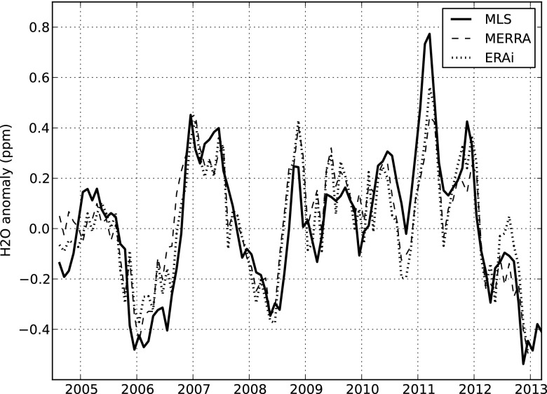
Fig. 1 shows monthly average tropical 82-hPa (∼18-km altitude) water-vapor volume-mixing–ratio anomalies observed by the Aura Microwave Limb Sounder (MLS) (16) (all tropical averages in this paper are over 30°N–30°S; anomalies are the remainder after the average annual cycle has been subtracted). These data are a good approximation of H₂O_ov-entry because this air has just entered the overworld and production of water from methane oxidation is negligible.

Fig. 1.

Time series of water vapor anomalies at 82 hPa (∼18 km), averaged over the latitudes 30°N–30°S. Data are from measurements made by the MLS (solid line). Dashed and dotted lines are reconstructions from multivariate regressions to the MLS data using different reanalysis estimates of BD and ΔT indices.

To better understand the observed variations in Fig. 1, we performed a multivariate linear regression on the data with the following regression model:

QBO is a quasibiennial oscillation index, for which we use the standardized anomaly of monthly and zonally averaged equatorial 50-hPa winds (17); BD is a Brewer–Dobson circulation index, for which we use the 82-hPa tropical heating rate anomaly as a surrogate; ΔT is the tropical average 500-hPa temperature anomaly, which is an index for the temperature of the tropical troposphere; and r is the residual. Values for the ΔT and BD indices are obtained from the Modern Era Retrospective-Analysis for Research and Applications (MERRA) (18) and the European Centre for Medium-Range Weather Forecasts interim reanalysis (ERAi) (19). See Methods for details about the regression.

Fig. 1 shows that the fits do an excellent job reproducing the MLS measurements (adjusted R² = 68% and 70% for the MERRA and ERAi fits, respectively). Table 1 lists the coefficients from regressions of the MLS data. Of particular note, the positive coefficient for the ΔT index supports a positive stratospheric water vapor feedback: an increase in tropospheric temperatures leads to higher H₂O_ov-entry, and because water vapor is a greenhouse gas, this leads to further warming of the troposphere.

Table 1.

Coefficients from regressions of the H₂O_ov-entry time series

Regressor	MLS observations		GEOSCCM simulations
	MERRA	ERAi	All variability	Long-term (>10 y) variations filtered out
QBO	0.09 ± 0.05	0.09 ± 0.04	N/A	N/A
BD	−3.9 ± 1.6	−2.6 ± 0.8	−6.1 ± 0.8	−6.4 ± 0.7
ΔT	0.27 ± 0.19	0.30 ± 0.16	0.36 ± 0.03	0.17 ± 0.08

The units of the QBO, BD, and ΔT coefficients are ppm, ppm/(K/d), ppm/K, respectively. The uncertainty is the 95% confidence interval. The two MLS fits use MERRA and ERAi values of BD and ΔT.

Climate Model Simulation of the Overworld.

We have also analyzed H₂O_ov-entry in version 2 of the Goddard Earth Observing System Chemistry Climate Model (GEOSCCM) (20). Here we look at a 21st century simulation driven by sea surface temperatures and other forcings from an A1B run of the National Center for Atmospheric Research Community Climate Model 3.0 (21).

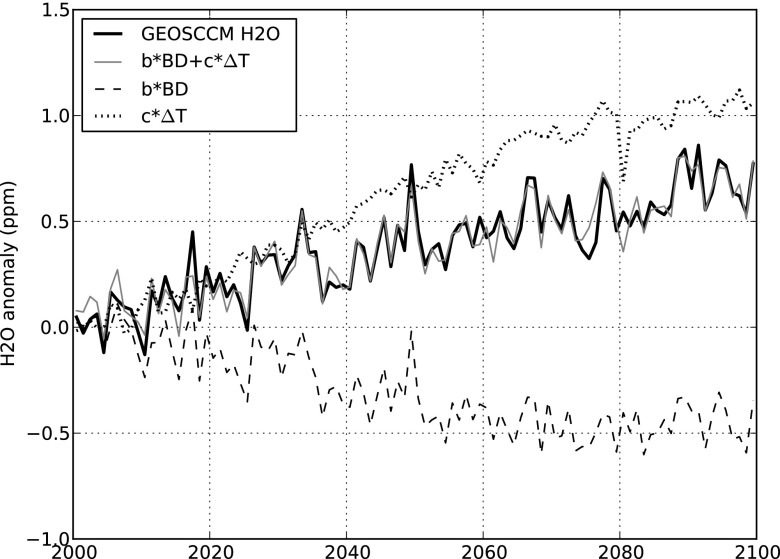
Fig. 2 shows annual-average 85-hPa tropical H₂O from the GEOSCCM (hereafter GEOSCCM H₂O_ov-entry) increases over the 21st century. To understand the factors underlying the GEOSCCM trend, we regress the GEOSCCM H₂O_ov-entry time series using the same regression model used to analyze the MLS data (Eq. 1). The BD and ΔT time series come from the GEOSCCM; the model does not have a QBO in it, so that process is excluded from the regression.

Fig. 2.

Time series of annual-average H₂O_ov-entry anomalies from the GEOSCCM (black) and the reconstruction from a multivariate least-squares regression (gray) over the 21st century. The dashed and dotted lines are the BD and ΔT terms of the regression, respectively.

Fig. 2 shows that the regression accurately reconstructs GEOSCCM H₂O_ov-entry. The individual components of the regression are also plotted and they show that the increasing H₂O_ov-entry over the 21st century is driven by warming of the troposphere (the ΔT term), which is partially offset by cooling of the TTL from an increase in the strength of the BD circulation (22, 23). The coefficients of the GEOSCCM regression are also listed in Table 1.

The climate variations in the MLS data are dominated by El Niño-Southern Oscillation (ENSO), whereas climate variation in the GEOSCCM is predominantly long-term warming. Because of this, we also perform regressions on GEOSCCM data filtered to remove variations with timescales >10 y, thereby emphasizing the short-term variations. These coefficients are also listed in Table 1 and, in general, this regression also produces results similar to the MLS regressions.

Lowermost Stratosphere.

Air in the lowermost stratosphere (hereafter, LMS) is a mixture of air that descended from the overworld, which went through the TTL, and air that crossed the extratropical tropopause, which is warmer than the tropical tropopause and therefore carries higher H₂O mixing ratios into the stratosphere (14).

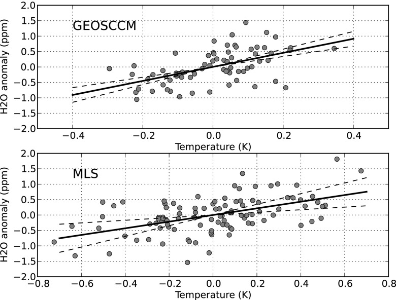
The factors that control LMS H₂O are not as well understood as for the overworld. We therefore apply the simplest test by regressing LMS H₂O anomalies against extratropical tropospheric temperatures anomalies. Fig. 3 shows a scatterplot of these quantities from the northern hemisphere. Overall, the GEOSCCM regressions yield slopes of 2.9 ± 0.1 and 1.9 ± 0.1 ppm/K in the northern and southern hemispheres, respectively. Regressions using time series filtered to remove variations with timescales >10 y produce slopes of 2.3 ± 0.6 and 1.7 ± 0.5 ppm/K.

Fig. 3.

Scatter plots of (Upper) GEOSCCM annual-average lowermost stratospheric H₂O (200-hPa mixing ratio, averaged between 50°N and 90°N) vs. extratropical tropospheric temperature (500-hPa temperature, averaged between 30°N and 90°N) and (Lower) the corresponding scatterplot of MLS monthly average H₂O vs. MERRA temperatures. For these plots, the GEOSCCM data have been filtered to remove long-term (>10 y) variations. The solid line is the least-squares fit, and the dashed lines are the 95% confidence interval.

Using MLS H₂O data and MERRA temperatures, the regression slopes are 1.1 ± 0.7 and 0.7 ± 0.5 ppm/K for the two hemispheres (results using ERAi temperatures are similar). Note that MLS H₂O mixing ratios in this region of the atmosphere are about half of the GEOSCCM’s (∼10 ppm vs. 20 ppm), so the regressions produce similar fractional changes in H₂O per unit of surface warming.

Both the MLS and GEOSCCM data indicate that LMS H₂O increases with increasing tropospheric temperatures, consistent with a positive LMS water vapor feedback. However, the details of the regression (e.g., latitude range to average over), although reasonable, are ultimately ad hoc because we do not have a good understanding of the processes that regulate LMS H₂O. More work is needed to strengthen our understanding of this issue.

Quantifying the Feedback.

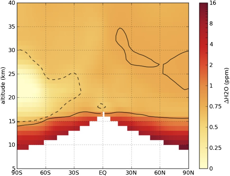
Fig. 4 plots the change in zonal average stratospheric H₂O in the GEOSCCM over the 21st century (hereafter, ΔH₂O). The contribution from CH₄ oxidation has been removed by assuming that each CH₄ molecule destroyed produces two H₂O molecules (24, 25). There is little variability in overworld ΔH₂O because stratospheric transport homogenizes the stratosphere much faster (∼5 y) than H₂O_ov-entry is changing over the 21st century. As a result, overworld ΔH₂O is everywhere approximately equal to the change in H₂O_ov-entry over the 21st century.

Fig. 4.

Change in zonal average stratospheric H₂O in ppm over the 21st century from the GEOSCCM; the contribution from methane oxidation has been subtracted. Note that the color scale is nonlinear; white areas indicate the troposphere. The dashed and solid lines are the 0.6 and 0.8 ppm contours, respectively.

An exception is the near-zero value over the South Pole at ∼22 km. This reflects the fact that the Antarctic stratosphere is near saturation during winter. Stratospheric cooling over the 21st century therefore increases condensation and irreversible loss of H₂O there, which on average cancels increasing H₂O_ov-entry. The rest of the stratosphere is so far above the frost point that it never saturates, so stratospheric cooling has no effect on H₂O.

Radiative transfer calculations are used to quantify the change in global average radiative flux at the tropopause due to the ΔH₂O field in Fig. 4. This calculation includes an adjustment to stratospheric temperatures using a fixed dynamical heating assumption (26). The calculated change in downward flux at the tropopause is +0.59 W/m². Dividing the change in flux by the change in global average surface temperature (2.0 K) yields a stratospheric water vapor feedback with a magnitude of +0.29 W/(m²⋅K).

Most of this feedback, however, comes from ΔH₂O in the LMS because the largest values of ΔH₂O are there and because the radiative impact of ΔH₂O maximizes just above the tropopause (10). To isolate the impact of changes in overworld ΔH₂O, we replace ΔH₂O in the LMS with 0.7 ppm, a value typical of the overworld. We then recalculate the change in downward flux at the tropopause to be +0.19 W/m², which in turn yields a feedback factor of +0.10 W/(m²⋅K).

Thus, one-third of the stratospheric water vapor feedback comes from increases in water vapor entering the stratosphere through the TTL, with the rest coming from increases in water vapor entering the LMS through the extratropical tropopause. The part of the feedback due to TTL processes is on firm footing because the GEOSCCM’s simulation of increasing H₂O_ov-entry is in good agreement with MLS observations, and the GEOSCCM results are typical of other chemistry–climate models with a well-resolved TTL and stratosphere (27). The LMS portion of the feedback, on the other hand, should be considered more preliminary because of limitations in our understanding of LMS H₂O.

This stratospheric water vapor feedback may be an important component of our climate system (28). A +0.1 W/(m²⋅K) feedback would be responsible for ∼10% or ∼0.4 K of the temperature response of a climate with an equilibrium climate sensitivity of 4 °C per doubled carbon dioxide. Because of nonlinearities in climate sensitivity, however, this same feedback would be responsible for ∼5% or ∼0.1 K of the temperature response for a climate with a sensitivity of 2 °C. The larger but more speculative feedback estimate of +0.3 W/(m²⋅K) would lead to contributions at least a factor of 3 larger.

Note that climate models uniformly project increases in stratospheric water vapor as the climate warms. For example, in a set of 16 Coupled Model Intercomparison Project Phase 5 (CMIP5) climate model simulations (29) of the 21st century driven by the RCP4.5 scenario, we found that the change in 70-hPa tropical H₂O over the 21st century ranges from 0.2 to 1.0 ppm. Thus, the stratospheric water vapor feedback is already operating—to some extent, at least—in climate models. However, differences in ΔH₂O among the models open the possibility of large differences among the models in this feedback. This might explain some of the spread in climate sensitivities among the models.

Methods

In the paper, we regressed the monthly MLS H₂O anomaly time series against a set of regressors that were previously identified as influencing H₂O_ov-entry. The regressors are monthly anomalies, calculated relative to the MLS data period. The regression is a standard linear least-squares multivariate regression and the regressors are lagged to account for the finite time it takes for the change in the indices to impact TTL temperatures and then to be felt at 82 hPa. The QBO index is lagged by 3 mo and the BD index and ΔT are lagged by 1 mo. Although each of these lags is physically reasonable, the exact lag is set to maximize the explained variance. For the LMS regressions, the maximum explained variance occurs with no lag between the time series.

The ENSO is an important driver of interannual variability in the climate system, but we omit it from Eq. 1 because our tropical tropospheric temperature regressor captures most of that variability. Likewise, whereas there are physical mechanisms by which QBO and BD may be correlated (30), the correlation is not statistically significant over the MLS period, and even over a longer time period the two are only weakly correlated (31).

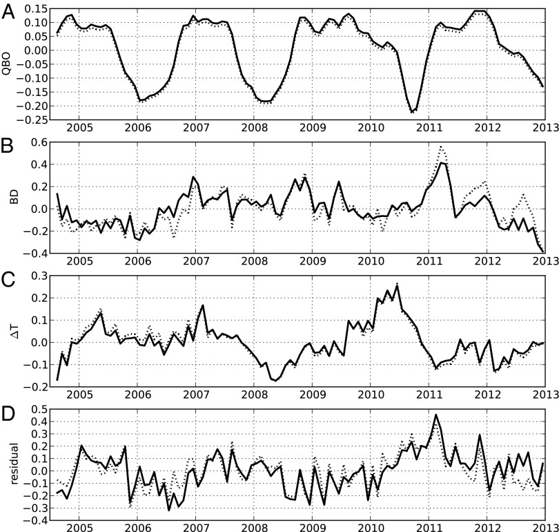
Fig. 5 shows time series of the components of the MLS regression. There is a clear QBO signal in H₂O_ov-entry (32–34). The strength of the BD circulation regulates upwelling in the TTL, which is inversely connected to TTL temperature anomalies (35). BD variations have previously been identified as an explanation for the drop in H₂O_ov-entry after 2000 (36, 37), and our analysis shows that a strengthening BD circulation contributed (along with the QBO) to a similar drop of H₂O_ov-entry during 2012. ΔT variations are responsible for H₂O_ov-entry variations of a few tenths of a ppm. Such variations are consistent with both simple arguments (38) and climate models (39) that suggest a warming climate will warm the tropopause. The residual shows some physical structure, suggesting that other processes may play a part in regulating stratospheric water vapor.

Fig. 5.

Components of the multivariate least-squares regression of the MLS observations. (A–C) Components of H₂O_ov-entry anomaly due to the QBO, BD, and ΔT; D shows the residual (all with units of ppm). The solid lines are from the regression using MERRA estimates of BD and ΔT, whereas the dotted lines are from the fit using ERAi estimates for the indices.

The GEOSCCM regression follows the same procedure as was used for the MLS regression, with two exceptions. First, the GEOSCCM has no QBO, so that term is set to zero. Second, the amplitude of the annual cycle in the GEOSCCM H₂O time series changes over the 21st century. This precludes the calculation of monthly interannual anomalies, so we instead analyze annual average GEOSCCM values in all regressions.

In estimating the uncertainty of the coefficients in regressions, one must account for autocorrelation in the time series, which reduces the number of degrees of freedom. Following Santer et al. (40), we estimate the number of degrees of freedom from the lag-1 autocorrelation of the residual time series. The adjusted number of degrees of freedom is then used in the estimate of the uncertainty of the coefficients.

The radiative calculations were done with the Atmospheric and Environmental Research (AER) Rapid Radiative Transfer Model (41, 42). This is a different radiative model than used by the GEOSCCM, but the GEOSCCM model agrees well with it in benchmarking studies (43). We assume here the efficacy of stratospheric water vapor is 1 (9). The unperturbed fields used in the radiative calculations are the 2000–2010 average from the GEOSCCM.

A monthly tropopause climatology, derived from MERRA data covering 2000–2012, is used in calculating the flux change at the tropopause. For a uniform increase in stratospheric H₂O of 1 ppm, we calculate a change in downward flux at the tropopause of +0.27 W/(m²⋅ppm), in good agreement with previous calculations (9, 10).

References

- 1.Soden BJ, Held IM. An assessment of climate feedbacks in coupled ocean-atmosphere models. J Clim. 2006;19(14):3354–3360. [Google Scholar]
- 2.Sherwood SC, Roca R, Weckwerth TM, Andronova NG. Tropospheric water vapor, convection, and climate. Rev Geophys. 2010;48(2) doi: 10.1029/2009rg000301. [DOI] [Google Scholar]
- 3.Minschwaner K, Dessler AE. Water vapor feedback in the tropical upper troposphere: Model results and observations. J Clim. 2004;17(6):1272–1282. [Google Scholar]
- 4.Forster PMD, Collins M. Quantifying the water vapour feedback associated with post-Pinatubo global cooling. Clim Dyn. 2004;23(2):207–214. [Google Scholar]
- 5.Soden BJ, Jackson DL, Ramaswamy V, Schwarzkopf MD, Huang X. The radiative signature of upper tropospheric moistening. Science. 2005;310(5749):841–844. doi: 10.1126/science.1115602. [DOI] [PubMed] [Google Scholar]
- 6.Dessler AE, Yang P, Zhang Z. Water-vapor climate feedback inferred from climate fluctuations, 2003-2008. Geophys Res Lett. 2008;35(20) doi: 10.1029/2008GL035333. [DOI] [Google Scholar]
- 7.Dessler AE, Wong S. Estimates of the water vapor climate feedback during the El Niño Southern Oscillation. J Clim. 2009;22(23):6404–6412. [Google Scholar]
- 8.Dessler AE. Observations of climate feedbacks over 2000-10 and comparisons to climate models. J Clim. 2013;26(1):333–342. [Google Scholar]
- 9.Forster PMD, Shine KP. Stratospheric water vapour changes as a possible contributor to observed stratospheric cooling. Geophys Res Lett. 1999;26(21):3309–3312. [Google Scholar]
- 10.Solomon S, et al. Contributions of stratospheric water vapor to decadal changes in the rate of global warming. Science. 2010;327(5970):1219–1223. doi: 10.1126/science.1182488. [DOI] [PubMed] [Google Scholar]
- 11.Stuber N, Ponater M, Sausen R. Is the climate sensitivity to ozone perturbations enhanced by stratospheric water vapor feedback? Geophys Res Lett. 2001;28(15):2887–2890. [Google Scholar]
- 12.Forster PMD, Shine KP. Assessing the climate impact of trends in stratospheric water vapor. Geophys Res Lett. 2002;29(6) doi: 10.1029/2001gl013909. [DOI] [Google Scholar]
- 13.Hoskins BJ. Towards a PV-θ view of the general circulation. Tellus. 1991;43AB(4):27–35. [Google Scholar]
- 14. Dessler AE, Hintsa EJ, Weinstock EM, Anderson JG, Chan KR (1995) Mechanisms controlling water vapor in the lower stratosphere: “A tale of two stratospheres.” J Geophys Res 100(D11):23167–23172.
- 15.Fueglistaler S, et al. The tropical tropopause layer. Rev Geophys. 2009;47(1) doi: 10.1029/2008RG000267. [DOI] [Google Scholar]
- 16.Read WG, et al. Aura Microwave Limb Sounder upper tropospheric and lower stratospheric H2O and relative humidity with respect to ice validation. J Geophys Res. 2007;112(D24) doi: 10.1029/2007jd008752. [DOI] [Google Scholar]
- 17. Climate Prediction Center (2013) QBO Index (NOAA Climate Prediction Center, College Park, MD). Available at www.cpc.ncep.noaa.gov/data/indices. Accessed September 18, 2013.
- 18.Rienecker MM, et al. MERRA – NASA’s modern-era retrospective analysis for research and applications. J Clim. 2011;24(14):3624–3648. doi: 10.1175/JCLI-D-16-0758.1. [DOI] [PMC free article] [PubMed] [Google Scholar]
- 19.Dee DP, et al. The ERA-Interim reanalysis: Configuration and performance of the data assimilation system. Q J R Meteorol Soc. 2011;137(656):553–597. [Google Scholar]
- 20.Pawson S, et al. Goddard Earth Observing System chemistry climate model simulations of stratospheric ozone-temperature coupling between 1950 and 2005. J Geophys Res. 2008;113(D12) doi: 10.1029/2007JD009511. [DOI] [Google Scholar]
- 21.Collins WD, et al. The Community Climate System Model version 3 (CCSM3) J Clim. 2006;19(11):2122–2143. [Google Scholar]
- 22.Butchart N, Scaife AA. Removal of chlorofluorocarbons by increased mass exchange between the stratosphere and troposphere in a changing climate. Nature. 2001;410(6830):799–802. doi: 10.1038/35071047. [DOI] [PubMed] [Google Scholar]
- 23.Garcia RR, Randel WJ. Acceleration of the Brewer-Dobson circulation due to increases in greenhouse gases. J Atmos Sci. 2008;65(8):2731–2739. [Google Scholar]
- 24.Le Texier H, Solomon S, Garcia RR. The role of molecular hydrogen and methane oxidation in the water vapour budget of the stratosphere. Q J R Meteorol Soc. 1988;114(480):281–295. [Google Scholar]
- 25.Dessler AE, et al. An examination of the total hydrogen budget of the lower stratosphere. Geophys Res Lett. 1994;21(23):2563–2566. [Google Scholar]
- 26.Fels SB, Mahlman JD, Schwarzkopf MD, Sinclair RW. Stratospheric sensitivity to perturbations in ozone and carbon-dioxide — radiative and dynamical response. J Atmos Sci. 1980;37(10):2265–2297. [Google Scholar]
- 27.Gettelman A, et al. Multimodel assessment of the upper troposphere and lower stratosphere: Tropics and global trends. J Geophys Res. 2010;115(D3) doi: 10.1029/2009jd013638. [DOI] [Google Scholar]
- 28.Joshi MM, Webb MJ, Maycock AC, Collins M. Stratospheric water vapour and high climate sensitivity in a version of the HadSM3 climate model. Atmos Chem Phys. 2010;10(15):7161–7167. [Google Scholar]
- 29.Taylor KE, Stouffer RJ, Meehl GA. An overview of CMIP5 and the experiment design. Bull Am Met Soc. 2012;93(4):485–498. [Google Scholar]
- 30.Plumb RA, Bell RC. A model of the quasi-biennial oscillation on an equatorial beta-plane. Q J R Meteorol Soc. 1982;108(456):335–352. [Google Scholar]
- 31.Davis SM, Liang CK, Rosenlof KH. Interannual variability of tropical tropopause layer clouds. Geophys Res Lett. 2013;40(11):2862–2866. [Google Scholar]
- 32.Giorgetta MA, Bengtsson L. Potential role of the quasi-biennial oscillation in the stratosphere-troposphere exchange as found in water vapor in general circulation model experiments. J Geophys Res. 1999;104(D6):6003–6019. [Google Scholar]
- 33.Geller MA, Zhou XL, Zhang MH. Simulations of the interannual variability of stratospheric water vapor. J Atmos Sci. 2002;59(6):1076–1085. [Google Scholar]
- 34.Randel WJ, Wu F, Gaffen DJ. Interannual variability of the tropical tropopause derived from radiosonde data and NCEP reanalysis. J Geophys Res. 2000;105(D12):15509–15523. [Google Scholar]
- 35.Yulaeva E, Holton JR, Wallace JM. On the cause of the annual cycle in tropical lower-stratospheric temperatures. J Atmos Sci. 1994;51(2):169–174. [Google Scholar]
- 36.Randel WJ, Wu F, Vomel H, Nedoluha GE, Forster P. Decreases in stratospheric water vapor after 2001: Links to changes in the tropical tropopause and the Brewer-Dobson circulation. J Geophys Res. 2006;111(D12) doi: 10.1029/2005JD006744. [DOI] [Google Scholar]
- 37.Dhomse S, Weber M, Burrows J. The relationship between tropospheric wave forcing and tropical lower stratospheric water vapor. Atmos Chem Phys. 2008;8(3):471–480. [Google Scholar]
- 38.Kirk-Davidoff DB, Hintsa EJ, Anderson JG, Keith DW. The effect of climate change on ozone depletion through changes in stratospheric water vapour. Nature. 1999;402(6760):399–401. [Google Scholar]
- 39.Gettelman A, et al. The tropical tropopause layer 1960-2100. Atmos Chem Phys. 2009;9(5):1621–1637. [Google Scholar]
- 40.Santer BD, et al. Statistical significance of trends and trend differences in layer-average atmospheric temperature time series. J Geophys Res. 2000;105(D6):7337–7356. [Google Scholar]
- 41.Mlawer EJ, Taubman SJ, Brown PD, Iacono MJ, Clough SA. Radiative transfer for inhomogeneous atmospheres: RRTM, a validated correlated-k model for the longwave. J Geophys Res. 1997;102(D14):16663–16682. [Google Scholar]
- 42. Mlawer EJ, Clough SA (1997) On the extension of rapid radiative transfer model to the shortwave region. Proceedings of the Sixth Atmospheric Radiation (ARM) Science Team Meeting (US Department of Energy, Washington, DC), pp 223–226.
- 43.Forster PM, et al. Evaluation of radiation scheme performance within chemistry climate models. J Geophys Res, 2011;116(D10) doi: 10.1029/2010jd015361. [DOI] [Google Scholar]