Increased dry-season length over southern Amazonia in recent decades and its implication for future climate projection

Significance

Whether the dry-season length will increase is a central question in determining the fate of the rainforests over Amazonia and the future global atmospheric CO₂ concentration. We show observationally that the dry-season length over southern Amazonia has increased significantly since 1979. We do not know what has caused this change, although it resembles the effects of anthropogenic climate change. The global climate models that were presented in the Intergovernmental Panel on Climate Change’s fifth assessment report seem to substantially underestimate the variability of the dry-season length. Such a bias implies that the future change of the dry-season length, and hence the risk of rainforest die-back, may be underestimated by the projections of these models.

Abstract

We have observed that the dry-season length (DSL) has increased over southern Amazonia since 1979, primarily owing to a delay of its ending dates (dry-season end, DSE), and is accompanied by a prolonged fire season. A poleward shift of the subtropical jet over South America and an increase of local convective inhibition energy in austral winter (June–August) seem to cause the delay of the DSE in austral spring (September–November). These changes cannot be simply linked to the variability of the tropical Pacific and Atlantic Oceans. Although they show some resemblance to the effects of anthropogenic forcings reported in the literature, we cannot attribute them to this cause because of inadequate representation of these processes in the global climate models that were presented in the Intergovernmental Panel on Climate Change’s Fifth Assessment Report. These models significantly underestimate the variability of the DSE and DSL and their controlling processes. Such biases imply that the future change of the DSE and DSL may be underestimated by the climate projections provided by the Intergovernmental Panel on Climate Change’s Fifth Assessment Report models. Although it is not clear whether the observed increase of the DSL will continue in the future, were it to continue at half the rate of that observed, the long DSL and fire season that contributed to the 2005 drought would become the new norm by the late 21st century. The large uncertainty shown in this study highlights the need for a focused effort to better understand and simulate these changes over southern Amazonia.

Fifteen percent of global photosynthesis occurs in the Amazon rainforest (1), where 25% of plant species are found (2). This rainforest ecosystem normally removes C from the atmosphere but released more than 1 Pg of C to the atmosphere in the 2005 drought (3). Consequently, even a partial loss of these forests would substantially increase global atmospheric CO₂ (4, 5) and reduce biodiversity. The dry-season length (DSL) is among the most important climate limitations for sustaining rainforests (6–9), especially in southern Amazonia, where rainforests are exposed to relatively long dry seasons and vulnerable to increasing conversion of native forests to cultivated crops (10–12). The extreme droughts in 2005 and 2010 had strong impacts on the rainforest and its C cycle (3, 13, 14). These unusual events, along with possible increase of drought severity and DSL during the past few decades (e.g., refs. 15 and 16) heighten the urgency of understanding what causes these dry anomalies and whether they will continue into the future. Contrary to the observed drying, some global climate models that previously projected strong drying over Amazonia now project much weaker drying by the end of the 21st century as these models evolve (17). Do these observed events represent the extremes of natural climate variability, or do climate projections underestimate potential future changes? This study explores one aspect of these questions by focusing on the change of DSL.

Evidence from Observations

Rain-gauge data from Amazonia are sparse and generally inadequate for assessing a trend in rainfall amounts. However, the dry-season end (DSE) over southern Amazonia is marked by a relatively rapid increase of rainfall on the order of 4–5 mm/d over areas of thousands of square kilometers during austral spring, and vice versa for the dry-season arrival (DSA) during austral fall (March–May) (18, 19). Hence, the timing of the DSA and DSE should be more clearly detectable by the rain-gauge network than the change in rainfall amount.

The DSL and DSE are derived from the National Oceanic and Atmospheric Administration (NOAA) Climate Prediction Center’s improved 1° gridded historical daily precipitation analysis over the Brazilian and Bolivian Amazon for the period of January 1978 to December 2007 (referred to as the Silva data; ref. 20) and the NOAA Climate Diagnostics Center’s 1° gridded daily precipitation data over the Brazilian and other northern Amazonian countries for the period of January 1940 to December 2011 (referred to as the recently updated SA24 data; ref. 21). These two regional daily rainfall datasets are based on ∼300–450 rain gauges that have been present throughout Amazonia (20, 21) for most of the time since 1979, more than those included in the global daily rainfall data (22). Both datasets show patterns of temporal variability, including their trends, similar to that obtained from the Global Precipitation Climatology Project (GPCP) monthly rainfall data and the Tropical Rainfall Measuring Mission (TRMM) satellite for the periods they overlap, although these regional rain gauge-based datasets show lower rainfall amounts compared with the satellite-based GPCP and TRMM (Fig. S1). The Silva dataset (20) has fewer rain gauges over the northeastern part of our southern Amazonian domain (5°–15°S, 50°–70°W), whereas the SA24 dataset (21) does not include rain gauges over the Bolivian Amazon, in the southwestern part of this domain. To mitigate such differences in the areas covered by rain gauges, we average these two rainfall datasets over each map cell for the period of 1979–2007 when they overlap and use SA24 for the period of 2008–2011 to form a merged daily rainfall dataset, referred to as the P_M data. For the period of January 1979–December 2011, daily rain rates of the P_M data are first spatially averaged over the southern Amazonian domain and then temporally averaged over a 5-d period (pentad) to reduce synoptic noise in estimating the DSA and DSE dates. The observed DSE is determined by the first date when the pentad mean rain rate changes from below to above the climatological annual mean rain rate of the same rainfall dataset during six out of eight pentads, and vice versa for the DSA (19). This definition captures the rapid transition from a lower to higher rainfall regime associated with the DSE, and vice versa for the DSA. The DSE and DSA are not influenced by any bias of rainfall amount, as long as the temporal patterns of the rainfall variation are not affected. Similar definitions have been widely used in the literature (18, 19, 23). For analysis of models, we modify our criterion to five out of eight pentads to best match the modeled DSE and DSA with observations.

The trends are computed using a least square fit. The confidence intervals and significance are determined based on the effective sample size and a t test, following Santer et al. (24). The trend significance is further tested by the right-tailed (positive) Vogelsang trend test, a more conservative test for strongly auto-correlated and nonstationary time series (25).

Fig. 1 shows the temporal variations of the DSL, DSE, and the mean rainfall during the dry-to-wet transition in austral spring season derived from the P_M dataset. The strong delay of the DSE in 2004 and 2005 is consistent with previous reports on the 2005 Amazonian drought (26, 27). The 2010 drought was mainly caused by strong rainfall reduction in early and middle 2010, followed by a rapid increase of rainfall at the end of October (16) (Fig. S2). Hence, the DSE in 2010 was not delayed. As shown in Table 1, the DSL has increased at a rate of 1.3 ± 0.5 pentad or about 6.5 ± 2.5 d per decade for uncertainties of P < 5% (24). This increase is mainly caused by a delay of the DSE at a rate of 0.9 ± 0.4 pentads or 4.5 ± 2.0 d per decade (P < 5%), as also evident in a decrease of rainfall by 0.19 ± 0.04 mm/d per decade (P < 5%) during austral spring. The more stringent Vogelsang test (25) still shows that these trends are significantly positive, but with uncertainty P < 10%. This delay of the DSE in recent decades is consistent with that inferred from a monthly rainfall dataset (16), the significant trends of decreasing rainfall at two long-term rain gauge stations located within our southern Amazonia domain (28), and also a decrease of convective cloudiness during austral spring detected by satellites (29). No significant changes of the DSA and rain rate are detected (Fig. S3).

Fig. 1.

(A) Annual time series of the DSL (red line) and DSE (blue line) dates derived from the P_M daily rainfall data over the southern Amazonian domain show a decrease of DSL due to a delay of DSE. The unit is pentad (5 d). On the left axis, the 55th pentad corresponds to September 2–7 of the calendar date and the 70th pentad corresponds to December 10–15. (B) Time series of austral spring seasonal rainfall over southern Amazonia derived from the P_M and GPCP datasets show decrease of rainfall consistent with the delay of DSE shown in (A). The linear trend is determined by a least-square fitting. Trends are significant at P < 5% based on Santer et al. (24).

Table 1.

The linear trends, confident interval and significance of the DSL and DSE for the periods 1979–2011 and 1979–2005

Data	DSL	DSE
PM (1979–2011)	1.3 ± 0.5 pen/dec	0.9 ± 0.4 pen/dec
	8.0 ± 2.5 d/dec	4.5 ± 2.0 d/dec
PM(1979–2005)	2.8 ± 0.6 pen/dec	2.3 ± 0.4 pen/dec
	14.0 ± 3.0 d/dec	11.5 ± 2.0 d/dec

Uncertainty less than 5% (P < 5%) as determined by the two-tailed t test with consideration of effective degree of freedom (24). The DSL and DSE are derived from the P_M merged daily rainfall data and the unit is pentads per decade (pen/dec) and days per decade (d/dec).

The main fire season over southern Amazonia spans the period of August–October, during the transition from the dry to the wet season. A delayed DSE would prolong the fire season, leading to an increase of fire counts during October and November. Thus, the latter measured by satellite can provide an independent verification of the former. Fig. 2 shows that a delay of the DSE is correlated with fire counts in the prolonged fire season (the correlation coefficient for the de-trended data is R = 0.83, P < 0.01, based on the method of ref. 30). Similarly, the correlation coefficient for the de-trended DSL and fire counts is 0.88, P < 0.01. This relationship is further supported by an increase of the McArthur Forest Fire Danger Index (FFDI, ref. 31), as determined from two independent atmospheric reanalysis products, the European Center for Medium Range Forecast Reanalysis (ERA)-Interim (32) and the National Center for Environment Prediction (NCEP) reanalyses (33). A high FFDI value represents a favorable meteorological condition for fire. These consistent changes between three physically related but independently obtained variables lend additional support to the observed delay of the DSE.

Fig. 2.

The DSE (unit is pentad) versus FFDI (green squares, units are nondimensional) and fire count (red circles, unit is number of pixels) in October and November for the period of 2000–2011 suggest prolonged fire season with delayed DSE. The 50th pentad corresponds to September 10–15 and the 70th pentad corresponds to December 10–15. The fire counts are derived from the moderate resolution imaging spectroradiometer fire-count data. FFDI is first derived from the ERA-Interim and NCEP reanalysis, respectively, and then averaged to obtain its values shown in the figure.

What could cause this delay of the DSE over southern Amazonia? Previous studies have established that stronger convective inhibition energy (CIN) and/or a poleward displacement of the subtropical jet over South America (SJ_SA) in austral winter are important contributors to an anomalously late DSE in austral spring (19, 34, 35). The former increases the work required to lift air near the surface to the level of free convection, above which the rising air becomes buoyant. The latter blocks cold-front incursions from the extratropics that would trigger rainfall over a large area and result in DSE (35). The influence of these preconditions on the DSE can be altered by random variations of the atmospheric circulation and oceanic circulations in austral spring. Such influences should be reduced by averaging over time, leading to more clear relationships between the SJ_SA, CIN, and DSE on a decadal scale than on an interannual scale. Fig. 3 shows that the delay of the DSE tends to occur when the SJ_SA is displaced poleward and CIN is relatively large. Likewise, an earlier DSE tends to occur when the SJ_SA is displaced equatorward and CIN is relatively low. Strong CIN combined with equatorward displacement of SJ_SA or low CIN with poleward SJ_SA do not seem to cause delay of the DSE, presumably because they compensate each other’s effects on the DSE. On a decadal scale, CIN increased in the 1990s relative to the 1980s (P < 5%, ref. 36). In the 2000s, CIN increased further from its values in the 1980s and 1990s, and SJ_SA becomes significantly more poleward. On an interannual scale, these connections between the SJ_SA, CIN, and DSE variations are less obvious, presumably owing to the influence on the DSE of random interannual variations of the tropical sea surface temperatures (SSTAs) and the Southern Annular Mode of the atmosphere in austral spring.

Fig. 3.

DSE date as a function of the latitudinal location of the SJ_SA and CIN in austral winter over southern Amazonia for the period of 1979–2011 suggests a preference of poleward SJ_SA and strong CIN by the delayed DSE. CIN and SJ_SA are first calculated using the inputs from ERA-Interim (ERAI) and NCEP reanalysis, respectively, then averaged to obtain the values shown in this figure. The triangle, square, and diamond symbols denote decadal means for the 1980s, 1990s, and 2000s. The error bars on these symbols represent the SEs with uncertainties of P < 5% (36).

What has caused the increase of CIN and poleward displacement of the SJ_SA? Most previous studies have linked change of rainfall over southern Amazonia to the Pacific Decadal Oscillation (PDO), changes of meridional SST gradient in the tropical Atlantic ocean associated with the Atlantic Multidecadal Oscillation (AMO, 26, 27, 37) and that of SJ_SA to the El Niño Southern Oscillation (ENSO) (35, 37). Because the periods of available rainfall data are too short to obtain significant correlations of these variables on a decadal scale, we evaluate the relationship between CIN, SJ_SA, and the SSTAs indices using their unfiltered de-trended time series for austral winter. Because the results are dominated by the interannual variations, the correlation coefficients between AMO and CIN may be weakened by strong interference from ENSO compared with those that might be obtained on a decadal scale from a longer record. The result indicates that CIN is marginally correlated with the PDO index (P = 8%, 30), whereas SJ_SA is not correlated with any of the ENSO, PDO, or AMO indices (Table S1). The lack of any robust correlation is consistent with the facts that (i) the SSTAs associated with ENSO, PDO, and AMO are generally weaker in austral winter and so are their influences on atmospheric circulation compared with austral summer or fall (38–40) and (ii) CIN is influenced by soil moisture anomalies, vegetation root depth, and lower troposphere temperature. Hence, any relationship with SSTAs is likely to be complex and nonlinear.

Could the decadal phase change of PDO and AMO qualitatively explain the change of CIN and SJ_SA? The PDO has been decreasing since the 1990s and became overall negative during 2000s. Such a change would not explain a poleward shift of SJ_SA (38) and an increase of CIN over southern Amazonia. AMO has shown a positive trend since 1979. However, the correlation between AMO and CIN is insignificant. Thus, natural interannual and decadal oceanic variability cannot be used to explain the changes of CIN and SJ_SA during the last few decades.

Could greenhouse effect-forced changes explain the increase of CIN and poleward shift of SJ_SA? Previous studies have established that the observed decreasing atmospheric temperature lapse rate and increasing surface temperature over the tropics during the past several decades are consistent with the “fingerprint” of the greenhouse effect (41). Over Amazonia, surface relative humidity has been decreasing owing to an increase of surface temperature over the past few decades (42). These changes could increase CIN, especially during winter (the dry season), when the surface air humidity cannot increase proportionally with temperature.

The poleward shift of SJ_SA can be contributed by both a globally poleward shift of the southern hemisphere subtropical jets (SJ_SH) and by the atmospheric planetary wave response to warm SSTAs over the central Pacific that is distinctively different from those induced by the ENSO and PDO (39, 43). In austral winter, the former is attributed to having been forced by the increase of greenhouse gases (43, 44), whereas the trend of the latter is attributed to having been forced by the warming of the central Pacific and Indian oceans in turn forced by greenhouse gases (39). The depletion of Antarctic ozone contributes importantly to the poleward shift of SJ_SH in austral summer and fall, but not in the winter season. It peaks in the middle stratosphere during austral spring (45) and its influence on atmospheric circulation propagates downward to the upper troposphere to influence the SJ_SH during austral summer. However, after the ozone hole recovers in austral fall, its effect becomes negligible for the austral winter (45). Hence, the observed changes of CIN and SJ_SA seem to be broadly consistent with those expected from forcing by greenhouse warming, and not a consequence of the ozone hole.

Land use can reduce land surface latent fluxes, and biomass burning aerosols can stabilize the atmospheric temperature stratification and weaken the dry-to-wet-season transition (46–49). Both could contribute to the delay of the DSE. However, long-term rain gauges and satellite observations show more clear decrease of rainfall and high clouds over the southwestern and northeastern parts of southern Amazonia where land use and fire are less prevalent than they are over the “Fire Arch” in southeastern Amazonia (28, 29). Furthermore, the DSE did not change before or after the 1991 Mount Pinatubo eruption (Fig. 1). Thus, what influence biomass burning aerosols and land use have on the observed delay of the DSE remains unclear beyond the observation that they do not seem to be the dominant cause.

Comparison with Climate Models

Attributing the changes of DSE, CIN, and SJ_SA to anthropogenic climate change and projecting their future changes require creditable climate models. Hence, we evaluate the 50 simulations provided by eight global climate models presented in the Intergovernmental Panel on Climate Change’s Fifth Assessment Report (IPCC AR5) based on the availability of their daily outputs of rainfall and other needed climate variables. These models are identified along with relevant information in Datasets and Methods and Table S2. The changes from the historical simulations of the global climate models that were presented in the IPCC AR5 are expected to be a result of random natural climate variability and appropriate anthropogenic and external forcing. If these models were perfect and the numbers of simulations were sufficient to generate a full spectrum of climate variability, one or more of these simulations would have captured the observed changes. Thus, the discrepancies between the models and observations should be caused either by undersampling of the possible changes owing to insufficient numbers of simulations or model errors, or both. Because the IPCC AR5 historical simulations end in 2005, we compare the observed changes for the period of 1979–2005 to the modeled 27-y changes in Fig. 4.

Fig. 4.

Distributions of the nonoverlapped 27-y trends of the DSE generated by the natural variability simulations (blue), historical simulations (red), and projections of future changes under the RCP8.5 scenario (green), respectively, suggest that the modeled DSE changes, including the projected future change, are significantly weaker than that which are observed during 1979–2005. The top 5% of the modeled trend samples are marked by blue, red, and green vertical dashed lines for the natural variability, historical simulations, and RCP8.5 scenario, respectively. The observed 27-y trend and confidence interval with uncertainties of P < 5% are marked by the black circle and horizontal bar in the upper right corner and are derived from the P_M daily rainfall data following method of Santer et al. (24).

The trend distribution of the simulations of natural variability is generated by 158 samples that represent nonoverlapped 27-y changes from a total of 4,266 y of simulation by multiple climate models. These simulations represent climate variability of the DSE changes for up to a few thousand years return period, and thus should adequately represent the range of the DSE natural variability for the time scale relevant to this study. The historical simulations by the eight climate models provide 40 samples of nonoverlapped 27-y changes for the period from the mid-19th century to 2005 and the climate projections under the Representative Concentration Pathway 8.5 scenario (RCP8.5) (50) provide 38 samples of the nonoverlapped 27-y changes for the period from 2006 up to 2299. Their ranges of the probability distributions are comparable to those represented by 158 samples of the natural variability simulations, despite their smaller number of samples. Thus, the differences between the statistical distribution of modeled changes and those observed should be mainly due to the models’ uncertainty, instead of due to under sampling of the climate variability.

Fig. 4 shows that all of the changes of the DSE during 27-y periods modeled by the natural climate variability, the historical simulations, and the RCP8.5 future scenario are significantly smaller than those observed, although the occurrences of delayed DSE trends increase with anthropogenic climate change. For example, the historical simulations, with realistic anthropogenic forcing, show an increased frequency of delayed trends of the DSE compared with those of the natural variability scenario, and more so for the RCP8.5 future scenario. However, these simulations do not produce any trends that are comparable to the large observed trend. The RCP8.5 scenario assumes that by 2100 the global anthropogenic radiative forcing would reach 8.5 Wm⁻² and that the atmospheric CO₂ concentration would become ∼1,360 ppm. However, the projected DSE changes are still significantly smaller than the observed DSE delay during the past 27-y period (with the uncertainty of P < 5%, Fig. 4). Because the change of the DSE dominates that of the DSL, the simulated and projected DSL changes are also significantly smaller than those observed (Fig. S4).

Why is there such a large discrepancy between modeled and observed changes of the DSE? Either the observed change of DSE during 1979–2005 represents an extremely large swing from natural variability with a return period greater than 4,000 y or the climate models underestimate the natural and forced climatic variability of the DSE. To explore the possibility of the latter, we show in Fig. 5 that no model could reproduce the observed relationship between the changes of DSE, SJ_SA, and CIN in any of their historical simulations. The majority of the simulations show much weaker changes of SJ_SA and CIN. These biases are consistent with the underestimation of SJ_SH variability reported in the literature (44) and the overestimation of the influences of the Pacific and Atlantic Intertropical Convergence Zones on Amazonia dry-season rainfall (51). The latter would undermine land-surface feedback and reduce the sensitivity of the CIN to land-surface warming and drying. Thus, the comparisons between historical simulations and observations suggest that the climate models evaluated in this study probably underestimate the sensitivity of the DSE, SJ_SA, and CIN to climate variability and anthropogenic change and that they could in turn underestimate potential future changes of the DSE and DSL over southern Amazonia (Fig. 4 and Figs. S4 and S5).

Fig. 5.

Distribution of the DSE trends (color shades) as a function of the trends of the SJ_SA (y axis) and CIN (x axis) in austral winter for the period of 1979–2005 derived from the historical simulations of the eight IPCC AR5 models (circles) is different from that which is observed (red square). The character in the center of each circle indicates the model’s name shown in Table S2. The ensemble mean of the eight models is indicated by the diamond symbol.

Implications

This study suggests that the IPCC AR5 models may underestimate the variability of the DSE (Fig. 4) and DSL (Fig. S4) over southern Amazonia and their sensitivity to the natural variability and anthropogenic forcing of the climate system. These biases could lead to an underestimate of the potential future climatic drying over southern Amazonia. However, one cannot simply extrapolate the observed changes to the future. Hence, we do not know how the DSL and DSE will change in the future without knowing what has caused their past changes. However, a risk of a future larger increase of DSL and delay of DSE does seem to be nonzero, as implied by its connection to the apparent influence of greenhouse-forced climate change on the CIN and SJ_SA. Although its risk is highly uncertain, such a future increase of the DSL would have strong impacts on southern Amazonia were it to occur. For example, if we assume that the DSL were to increase at half of the rates we observed during 1979–2011, the DSL would be about 1 ± 1/3 mo longer by 2090 than that in the 2000s. Consequently, the long DSL and fire season during the 2004–2005 drought would become the new norm (Fig. 2). Given the observed slow recovery of the rainforests after the 2005 drought (14), these changes could greatly increase the danger of a transition from a rainforest to a savanna regime over southern Amazonia (10, 12, 52), especially with the longer DSL coupled to the higher surface temperatures and more fragmented forests expected in the future (11, 12, 53), and even accounting for the increase of dry season resilience of the rainforest in an elevated CO₂ environment (17). Given such potential impacts on the global and regional C cycle and biodiversity, the large uncertainty in determining future changes of the DSL and DSE shown by this study highlights the importance and urgency of better monitoring and understanding the changes of the dry season over southern Amazonia. In addition to the impact of global climate forcing, the roles that regional biomass burning and land use play in the DSL over southern Amazonia also need to be clarified.

Datasets and Methods

The CIN, SJ_SA, and FFDI are all derived from the ERA-Interim and the NCEP reanalyses. CIN in Fig. 3 is computed from 6-h temperature, humidity, and geopotential height profiles. In Fig. 5, a CIN index (54) is used because the models do not provide the instantaneous temperature and humidity profiles needed for computing CIN. The latitude of the SJ_SA is determined by the equatorward latitudinal location of the 28 m⋅s⁻¹ monthly zonal wind contour at 200 hPa between 30°and 90°W. This index most consistently captures the latitudinal variation of the SJ_SA associated with tropical meridional circulation changes in the two reanalysis products, although the use of other similar zonal wind indices does not change the variations of the SJ_SA. The variation of SJ_SA based on this index is consistent with those determined by the zero stream function in latitudinal-height space and the 250 W⋅m⁻² Outgoing Longwave Radiation Contour (55) used in the literature to describe changes of global subtropical jets. The FFDI (31) is computed as

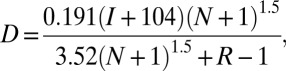where T is the daily maximum temperature (°C), H is the daily minimum relative humidity (%), W is the daily mean wind speed at 10 m (km/h), N is the number of days since the last rain, R is the total rainfall (mm) in the most recent 24 h with rain, and I is the total rainfall (mm) needed to restore the soil moisture content to 200 mm. These inputs are provided by the 6-h outputs from the ERA-Interim and NCEP reanalysis. Fire count is obtained from the moderate resolution imaging spectroradiometer on board the National Aeronautics and Space Administration (NASA) aqua satellite (56) (ftp://fire:burnt@fuoco.geog.umd.edu/).

The AMO index is obtained from www.esrl.noaa.gov/psd/data/timeseries/AMO/. The PDO index is obtained from http://jisao.washington.edu/pdo/PDO.latest. The Niño3 and Niño4 indices are obtained from www.esrl.noaa.gov/psd/data/climateindices/list/.

Eight of the climate models that were part of the IPCC AR5 are used in this study based on availability of the daily outputs of precipitation and other needed climate variables. These models are the National Center for Atmospheric Research Community Climate System Model Version 4 (CCSM4), the NOAA Geophysical Fluid Dynamics Laboratory Climate Model Version 3 (GFDL-CM3), the Earth System Model (GFDL-ESM2M), the NASA Goddard Institute for Space Studies (GISS)-E2-H and GISS-E2-R models, the United Kingdom Met Office Hadley Center (HadGEM2-CC and HadGEM2-ES) models, and the Max Planck Institute for Meteorology (MPI-ESM-LR) model. All of the model output and observational datasets are remapped to the 2.5° latitude and longitude grids when they are compared with each other in Figs. 4 and 5. A brief summary of model resolutions, available ensemble simulations and sources of the models are provided in Table S2.

References

- 1.Field CB, Behrenfeld MJ, Randerson JT, Falkowski P. Primary production of the biosphere: Integrating terrestrial and oceanic components. Science. 1998;281(5374):237–240. doi: 10.1126/science.281.5374.237. [DOI] [PubMed] [Google Scholar]
- 2.Dirzo R, Raven PH. Global state of biodiversity and loss. Annu Rev Environ Resour. 2003;28(1):137–167. [Google Scholar]
- 3.Phillips OL, et al. Drought sensitivity of the Amazon rainforest. Science. 2009;323(5919):1344–1347. doi: 10.1126/science.1164033. [DOI] [PubMed] [Google Scholar]
- 4.Cox PM, Betts RA, Jones CD, Spall SA, Totterdell IJ. Acceleration of global warming due to carbon-cycle feedbacks in a coupled climate model. Nature. 2000;408(6809):184–187. doi: 10.1038/35041539. [DOI] [PubMed] [Google Scholar]
- 5.Fung IY, Doney SC, Lindsay K, John J. Evolution of carbon sinks in a changing climate. Proc Natl Acad Sci USA. 2005;102(32):11201–11206. doi: 10.1073/pnas.0504949102. [DOI] [PMC free article] [PubMed] [Google Scholar]
- 6.Sombroek W. Spatial and temporal patterns of Amazon rainfall. AMBIO. 2001;30(7):388–396. doi: 10.1579/0044-7447-30.7.388. [DOI] [PubMed] [Google Scholar]
- 7.Da Silveira Lobo Sternberg L. Savanna–forest hysteresis in the tropics. Glob Ecol Biogeogr. 2001;10(4):369–378. [Google Scholar]
- 8.Hutyra LR, et al. Climatic variability and vegetation vulnerability in Amazônia. Geophys Res Lett. 2005;32(24):L24712. [Google Scholar]
- 9.Staver AC, Archibald S, Levin SA. The global extent and determinants of savanna and forest as alternative biome states. Science. 2011;334(6053):230–232. doi: 10.1126/science.1210465. [DOI] [PubMed] [Google Scholar]
- 10.Oyama MD, Nobre CA. A simple potential vegetation model for coupling with the simple biosphere model (SIB) Rev Bras Meteorol. 2004;1(2):203–216. [Google Scholar]
- 11.Salazar LF, Nobre CA, Oyama MD. Climate change consequences on the biome distribution in tropical South America. Geophys Res Lett. 2007;34(9):L09708. [Google Scholar]
- 12.Malhi Y, et al. Exploring the likelihood and mechanism of a climate-change-induced dieback of the Amazon rainforest. Proc Natl Acad Sci USA. 2009;106(49):20610–20615. doi: 10.1073/pnas.0804619106. [DOI] [PMC free article] [PubMed] [Google Scholar]
- 13.Lewis SL, Brando PM, Phillips OL, van der Heijden GM, Nepstad D. The 2010 Amazon drought. Science. 2011;331(6017):554. doi: 10.1126/science.1200807. [DOI] [PubMed] [Google Scholar]
- 14.Saatchi S, et al. Persistent effects of a severe drought on Amazonian forest canopy. Proc Natl Acad Sci USA. 2013;110(2):565–570. doi: 10.1073/pnas.1204651110. [DOI] [PMC free article] [PubMed] [Google Scholar]
- 15.Li W, Fu R, Dickinson RE. Rainfall and its seasonality over the Amazon in the 21st century as assessed by the coupled models for the IPCC AR4. J Geophys Res. 2006;111(D2):D02111. [Google Scholar]
- 16.Marengo JA, et al. The drought of 2010 in the context of historical droughts in the Amazon region. Geophys Res Lett. 2011;38:L12703. [Google Scholar]
- 17.Good P, Jones C, Lowe J, Betts R, Gedney N. Comparing Tropical Forest Projections from Two Generations of Hadley Centre Earth System Models, HadGEM2-ES and HadCM3LC. J Clim. 2013;26(2):495–511. [Google Scholar]
- 18.Marengo JA, Liebmann B, Kousky VE, Filizola NP, Wainer IC. Onset and end of the rainy season in the Brazilian Amazon basin. J Clim. 2001;14(5):833–852. [Google Scholar]
- 19.Li WH, Fu R. Transition of the large-scale atmospheric and land surface conditions from the dry to the wet season over Amazonia as diagnosed by the ECMWF re-analysis. J Clim. 2004;17(13):2637–2651. [Google Scholar]
- 20.Silva VBS, Kousky VE, Shi W, Higgins RW. An improved gridded historical daily precipitation analysis for Brazil. J Hydrometeorol. 2007;8(4):847–861. [Google Scholar]
- 21.Liebmann B, Allured D. Daily precipitation grids for South America. Bull Am Meteorol Soc. 2005;86(11):1567. [Google Scholar]
- 22.Menne MJ, Durre I, Vose RS, Gleason BE, Houston TG. An overview of the Global Historical Climatology Network-Daily Database. J Atmos Ocean Technol. 2012;29(7):897–910. [Google Scholar]
- 23.Kousky VE. Pentad outgoing longwave radiation climatology for the South American sector. Rev Bras Meteor. 1988;3:217–231. [Google Scholar]
- 24.Santer BD, et al. Statistical significance of trends and trend differences in layer-average atmospheric temperature time series. J Geophys Res. 2000;105(6):7337–7356. [Google Scholar]
- 25.Fomby TB, Timothy JV. The application of size-robust trend statistics to global-warming temperature series. J Clim. 2002;15:117–123. [Google Scholar]
- 26.Zeng N, et al. Causes and impacts of the 2005 Amazon drought. Environ Res Lett. 2008;3(1):014002. [Google Scholar]
- 27.Fernandes K, et al. North Tropical Atlantic influence on western Amazon fire season variability. Geophys Res Lett. 2011;38(12):L12701. [Google Scholar]
- 28.Satyamurty P, et al. Rainfall trends in the Brazilian Amazon basin in the past eight decades. Theor Appl Climatol. 2010;99:139–148. [Google Scholar]
- 29.Arias PA, Fu R, Hoyos CD, Li W, Zhou L. Changes in cloudiness over the Amazon rainforests during the last two decades: Diagnostic and potential causes. Clim Dyn. 2011;37(5-6):1151–1164. [Google Scholar]
- 30.Bretherton CS, Widmann M, Dymnikov VP, Wallace JM, Blade I. The effective number of spatial degrees of freedom of a time-varying field. J Clim. 1999;12(7):1990–2009. [Google Scholar]
- 31. Golding N, Betts R (2008) Fire risk in Amazonia due to climate change in the HadCM3 climate model: Potential interactions with deforestation. Global Biogeochem Cycles 22(4):GB4007.
- 32.Dee DP, et al. The ERA-Interim reanalysis: Configuration and performance of the data assimilation system. Q J R Meteorol Soc. 2011;137(656):553–597. [Google Scholar]
- 33.Kalnay E, et al. The NCEP/NCAR 40-year reanalysis project. Bull Am Meteorol Soc. 1996;77(3):437–471. [Google Scholar]
- 34.Fu R, Zhu B, Dickinson RE. How do atmosphere and land surface influence seasonal changes of convection in the tropical Amazon? J Clim. 1999;12(5):1306–1321. [Google Scholar]
- 35.Li WH, Fu R. Influence of cold air intrusions on the wet season onset over Amazonia. J Clim. 2006;19(2):257–275. [Google Scholar]
- 36.Hogg RV, Ledolter J. Engineering Statistics. New York: MacMillan; 1987. [Google Scholar]
- 37.Pezza AB, Ambrizzi T. Dynamical conditions and synoptic tracks associated with different types of cold surges over tropical South America. Int J Climatol. 2005;25:215–241. [Google Scholar]
- 38.Pezza AB, Durrant T, Simmonds I, Smith I. Southern Hemisphere synoptic behavior in extreme phases of SAM, ENSO, sea ice extent, and southern Australia rainfall. J Clim. 2008;21(21):5566–5584. [Google Scholar]
- 39.Ding Q, Steig EJ, Battisti DS, Ku¨ttel M. Winter warming in West Antarctica caused by central tropical Pacific warming. Nat Geosci. 2011;4:398–403. [Google Scholar]
- 40.Chen Y, Velicogna I, Famiglietti JS, Randerson JT. Satellite observations of terrestrial water storage provide early warning information about drought and fire season severity in the Amazon. J Geophys Res Biogeosci. 2013;118:495–504. [Google Scholar]
- 41.Santer BD, et al. Consistency of modelled and observed temperature trends in the tropical troposphere. Int J Climatol. 2008;28:1703–1722. [Google Scholar]
- 42.Dai A. Recent climatology, variability, and trends in global surface humidity. J Clim. 2006;19(15):3589–3606. [Google Scholar]
- 43.Deser C, Phillips AS. Atmospheric circulation trends, 1950-2000: The relative roles of sea surface temperature forcing and direct atmospheric radiative forcing. J Clim. 2009;22(2):396–413. [Google Scholar]
- 44.Lu J, Vecchi GA, Reichler T. Expansion of the Hadley cell under global warming. Geophys Res Lett. 2007;34(6):L06805. [Google Scholar]
- 45.Thompson DW, et al. Signatures of the Antarctic ozone hole in Southern Hemisphere surface climate change. Nat Geosci. 2011;4(11):741–749. [Google Scholar]
- 46.Zhang Y, et al. A regional climate model study of how biomass burning aerosol impacts land-atmosphere interactions over the Amazon. J Geophys Res. 2008;113(D14):D14S15. [Google Scholar]
- 47.Bevan SL, North PRJ, Grey WMF, Los SO, Plummer SE. Impact of atmospheric aerosol from biomass burning on Amazon dry-season drought. J Geophys Res. 2009;114(D9):D09204. [Google Scholar]
- 48.Costa MH, Pires GF. Effects of Amazon and Central Brazil deforestation scenarios on the duration of the dry season in the arc of deforestation. Int J Climatol. 2010;30(13):1970–1979. [Google Scholar]
- 49.Lee JE, Lintner BR, Boyce CK, Lawrence PJ. Land use change exacerbates tropical South American drought by sea surface temperature variability. Geophys Res Lett. 2011;38(19):L19706. [Google Scholar]
- 50.van Vuuren DP, Lucas PL, Hilderink H. Downscaling drivers of global environmental change: Enabling use of global SRES scenarios at the national and grid levels. Glob Environ Change. 2007;17(1):114–130. [Google Scholar]
- 51. Yin L, Fu R, Shevliakova E, Dickinson RE (2012) How well can CMIP5 simulate precipitation and its controlling processes over tropical South America? Clim Dyn, 10.1007/s00382-012-1582-y.
- 52.Hoffmann WA, Orthen B, Nascimento PKV. Comparative fire ecology of tropical savanna and forest trees. Funct Ecol. 2003;17(6):720–726. [Google Scholar]
- 53.Soares-Filho BS, et al. Modelling conservation in the Amazon basin. Nature. 2006;440(7083):520–523. doi: 10.1038/nature04389. [DOI] [PubMed] [Google Scholar]
- 54.Myoung B, Nielsen-Gammon JW. The convective instability pathway to warm season drought in Texas. Part I: The role of convective inhibition and its modulation by soil moisture. J Clim. 2010;23(17):4461–4473. [Google Scholar]
- 55.Hu Y, Fu Q. Observed poleward expansion of the Hadley circulation since 1979. Atmos Chem Phys. 2007;7(19):5229–5236. [Google Scholar]
- 56. Giglio L (2010) MODIS Collection 5 Active Fire Product User’s Guide: Version 2.4. Available at http://www.fao.org/fileadmin/templates/gfims/docs/MODIS_Fire_Users_Guide_2.4.pdf.
Associated Data
This section collects any data citations, data availability statements, or supplementary materials included in this article.