Three-dimensional reconstruction of icosahedral particles from single micrographs in real time at the microscope

Abstract

Single particle analysis is a valuable tool in cryo-electron microscopy for determining the structure of biological complexes. However, the conformational state and the preparation of the sample are factors that play a critical role in the ultimate attainable resolution. In some cases extensive analysis at the microscope of a sample under different conditions is required to derive the optimal acquisition conditions. Currently this analysis is limited to raw micrographs, thus conveying only limited information on the structure of the complex.

We are developing a computing system that generates a three-dimensional reconstruction from a single micrograph acquired under cryogenic and low dose conditions, and containing particles with icosahedral symmetry. The system provides the microscopist with immediate structural information from a sample, while it is in the microscope and during the preliminary acquisition stage. The system is designed to run without user intervention on a multi-processor computing resource and integrates all the processing steps required for the analysis. Tests performed on experimental data sets show that the probability of obtaining a reliable reconstruction from one micrograph is primarily determined by the quality of the sample, with success rates close to 100% when sample conditions are optimal, and decreasing to about 60% when conditions are sub-optimal. The time required to generate a reconstruction depends significantly on the diameter of the particles, and in most instances takes about one minute. The proposed approach can provide valuable three-dimensional information, albeit at low resolution, on conformational states, epitope binding, and stoichiometry of icosahedral multi-protein complexes.

1. Introduction

Transmission electron microscopy (TEM), combined with image analysis and three-dimensional (3D) image processing, is rapidly evolving as a reliable and essential tool for structural biologists to study the 3D structures of macromolecular complexes under near native conditions (Frank, 2006). High-resolution models of such complexes can be obtained by combining images of thousands to upwards of millions of particles, after having determined their orientations in the acquired images by single particle analysis (Zhou, 2011). Technological advancements in the fabrication of microscopes and detector devices enable the acquisition of high quality micrographs at increased speed (Bammes et al., 2012; Yu et al., 2011), and several software packages are available to automate the acquisition process (Korinek et al., 2011; Suloway et al., 2005).

Despite all this progress, the quality of the biological sample and the way it is prepared for the microscopic analysis are still the predominant factors that determine the ultimate resolution achievable for the final structure (Jensen, 2010). As a first requirement the particles in the sample need to be intact and homogeneous, both in terms of protein composition and conformational state, otherwise additional layers of processing are required to separate the different populations. When a complex is experimentally bound to an additional component, such as viruses decorated with fragment antibodies (Fabs), it is desirable to achieve stoichiometric binding in order to optimize analysis of interactions between the two. Furthermore, the preparation of a sample for cryo-electron microscopy is a multi-step process in which each step must be enhanced for the biological complex under study. Therefore, the preparation always requires some level of decision by the microscopist, and this will affect the quality of the reconstruction. Composition of the buffer, treatment applied to the support film of the TEM grids, and the vitrification procedure are just three examples of factors that can require extensive trial and error experimentation. Part of the analysis of a sample under different preparation conditions is usually conducted at the microscope and involves the acquisition of some images and their visual inspection in two dimensions, using the imaging tools provided by the acquisition software. However, evaluation based on the analysis of 2D images provides only partial information about the properties of the specimen (e.g. particle integrity and concentration, ice thickness, etc.) or the micrograph (e.g. the level of defocus and astigmatism, presence of specimen drift or charging, etc.). As a solution for the analysis of particles with icosahedral symmetry, we have developed a system that takes images as they are acquired at the microscope and processes them on a high-performance computing platform. The goal is to provide the microscopist with immediate 3D structural information about particles in a sample while it is in the microscope and during the preliminary acquisition stage. Each successive micrograph is analyzed independently and a 3D reconstruction is computed from the particles available in that image, within the time typically required to move the sample to a new field of view and to record the next image. To maximize the benefits of such a system to the microscopist, we have designed it so that no user intervention is required other than to establish an initial configuration, and this can be accomplished quite easily and with very little training.

To our knowledge a similar approach has thus far been explored with electron tomography (Zheng et al., 2007), where the goal is to generate in an automated fashion a tomogram immediately after an entire tilt series is acquired. Current computational efforts on automation in single particle analysis mostly focus only on single aspects of the entire processing procedure, with minimal efforts on integration. For example, an area under active development involves streamlining the acquisition procedure to optimize time at the microscope while providing high-throughput data (Korinek et al., 2011; Shi et al., 2008; Suloway et al., 2005). All the processing steps required for obtaining a 3D reconstruction, such as particle picking, contrast transfer function (CTF) estimation, and particle orientation determination have been extensively analyzed, and methods proposed to automate each step have been described (e.g. Adiga et al., 2005; Mallick et al., 2005; Ogura and Sato, 2004; Vargas et al., 2013; Voss et al., 2009). However, an integrated approach for real time operation has yet to be demonstrated. Here we present a system that we are developing that provides timely 3D feedback to the microscopist while the sample is inside the microscope. We describe all of the components of our system and demonstrate its performance on experimental micrographs of icosahedrally-symmetric particles. Tests have been performed on existing data sets, chosen as representative of different acquisition conditions.

2. Approach

2.1 Overview and specifications

The general concept of a real-time 3D reconstruction at the microscope protocol is to analyze a micrograph as soon as it is acquired, with the goal of determining a reliable, albeit low resolution 3D reconstruction of the particles available in that micrograph. In this way the microscopist can get immediate visual feedback about the structure of the sample while it is in the microscope. The image processing procedures are designed to accelerate and not interfere with the work of the microscopist, since all the analysis is performed in an automated fashion with minimal user intervention. Also, all the results from the analysis are visually accessible, without any need to interact with the program unless desired. The microscopist is expected to get the structural information derived from one micrograph before acquiring the next micrograph from a different area of the specimen. In general, the time required to acquire manually two successive micrographs from different regions of a vitrified sample takes at least a minute or two, which depends on sample conditions (e.g. particle concentration and ice thickness) and microscope configuration.

2.2 Workflow

A sequential set of processing steps must be performed to generate a 3D reconstruction from a set of particles imaged in a micrograph (Figure 1). These steps are common to those needed during single particle analysis of an entire data set of images, with the exception that only one micrograph is analyzed in this case.

Figure 1.

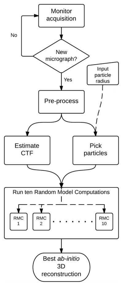
Automated reconstruction workflow. The system continuously monitors if micrographs are acquired, and new images are immediately added to the queue for processing. The only input parameter required from the user at the beginning of the procedure is the radius of the particle. Pre-processing involves making two copies of the micrograph binned at different sizes and format conversion. These copies are then processed in parallel to estimate the microscope CTF and to pick the particles from the available field of view. Once the particle images are extracted and the microscope acquisition parameters (astigmatism, defocus) are available, a set of ten separate RMCs is launched. These models are iteratively refined in parallel, on separate processors, and the final 3D reconstruction results are compared to select the best reconstruction.

The images acquired at the microscope are stored in a file directory, usually defined by the user, on a compute server separate from the microscope. This directory is constantly monitored for acquisition of new micrographs. The only information needed to start the processing is the name of this directory and an approximate radius of the particles in the sample.

2.2.1 Defocus estimation and particle picking

Once a new image is acquired and stored as a file, two copies of it, at different levels of pixel binning, are generated in a working directory. One copy, binned by a factor of 2, is used to estimate the defocus and astigmatism of the micrograph and is then deleted. Defocus and astigmatism are estimated with the program CTFFIND3, ver. 3.4 (Mindell and Grigorieff, 2003), which performs periodogram averaging using a window size of 128² pixels. The default search range for the defocus determination is set from 0.8 to 4 μm underfocus. The output defocus and astigmatism values are stored on file for each micrograph. The second copy of the micrograph, which is used for all the remaining processing steps, is binned according to the resolution set as target for the reconstruction. In order to reduce the computational time while making sure that the target resolution doesn’t approach too close to the Nyquist limit, the level of binning was set to give a pixel size at least four times smaller than the target resolution. Hence, for the target value of 28 Å that we used in our experiments, this translates to a final pixel size at most of 5.5 Å. Individual particle images are located in the micrograph using a heuristic algorithm based on the Crosspoint method (Boier Martin et al., 1997) and implemented in RobEM. (http://cryoem.ucsd.edu/programs.shtm). Some steps of the algorithm have been optimized in order to improve the detection efficiency (Appendix). The only input parameter required by the program is the radius of the particle. The size of the box extracted around each particle located is set to three times the radius. After being extracted from the micrograph, the density values of the boxed particles are floated and normalized, and their edges are apodized, using routines available in Auto3DEM (Yan et al., 2007b).

2.2.2 Ab-initio reconstruction

All the particle images extracted from the micrograph are used to compute a 3D density map without using a reference model. Since the particles are assumed to have icosahedral symmetry, we use the Random Model Computation (RMC) Method (Yan et al., 2007a), as implemented in Auto3DEM. Specifically, ten initial random models are obtained by assigning ten different sets of random orientations to all the particle images and a first 3D reconstruction is computed from each independent set. Each resulting reconstruction is then independently refined by running ten iterations of alignment, using a variant of the projection matching approach that is based on the Polar Fourier Transform method (Baker and Cheng, 1996). The angular step interval (in degrees) used in defining the search grid for the alignment is specifically adjusted for each dataset, using the formula (180d)/(2πr), where d and r are the target resolution and particle radius (in Å), respectively. This particular choice means that the search space is probed with reference projections that are incrementally displaced by half the nominal resolution, and with our settings provided a balance between accuracy of the final map and computational cost involved in the projection matching computations. The target resolution is set to 28 Å and the particle radius is that input by the user before starting the monitoring process. The range of radii to consider for projection matching is determined in an adaptive manner, at each iteration, from the radial profile of the current reconstruction. The metric used for determining the range is based in part on the variance of the radial profile (Cardone et al., in preparation). A variation of this metric is used also to decide which reconstruction, among the ten that are obtained after completion of the ten iterations, is selected as the best candidate to represent the particles analyzed.

2.3 Implementation

We developed a single program, AutoRTM, whose task is to generate 3D reconstructions in real-time from a single acquired micrograph. The program depends on Auto3DEM for carrying out all the single steps of processing, like CTF estimation, particle picking, and RMC, and it implements the streamlining and automation of all the operations, and includes a graphical interface for monitoring the progress (Figure 2). It is written mostly in python, and relies on library modules generally available on Linux and Mac OSX platforms.

Figure 2.

Graphical user interface of AutoRTM. Acquired images are displayed as soon as they are available, usually within two seconds, at the left side of the interface window. Particles picked by the program are highlighted with red circles. The incoherent Fourier Transform calculated from the acquired image and a simulated Contrast Transfer Function are displayed at the top-center of the interface window at left and right sides, respectively. Just below this split display, a central, 1-pixel thick section from the 3D reconstruction selected as the best of the ten candidate reconstructions is shown. At the top-right of the interface window, under the Micrograph tab, are various control buttons that allow the microscopist to view previous results along with quantitative information on the results of the processing. These include the number of particles picked, and the estimate of the defocus values along the minimum and the maximum axes. Initial settings, such as the estimated particle radius and the name of the directory that is constantly monitored for new images, are specified under the Session tab. Central sections from all ten candidate reconstructions can be inspected by opening an additional window, shown at the bottom.

The software is organized into two modular layers. The first, written in Perl scripting language, controls the actual processing of each micrograph, and it can be launched as a stand-alone program. This feature is available primarily for testing purposes. A second layer, written in Python language, is responsible for all monitoring activities and it provides a graphical interface for user interaction. With this interface, the user can verify the results by visually inspecting several different representations of the processed data, including the micrograph, the locations of particles picked, the power spectrum of the micrograph and a simulated CTF, and a central cross-section of the best reconstruction from the particles (Figure 2). Optionally, one may also view corresponding sections of all ten reconstructions generated by the RMC. All the images displayed are generated using conversion programs available in Bsoft (Heymann and Belnap, 2007).

In order to comply with the requirements of generating a reconstruction within a few minutes after acquisition of a micrograph, some parallelism was introduced in the processing. Since particle picking and CTF estimation are both performed on the input micrograph but because they involve independent computations, they are run in parallel. The program (RobEM) that performs particle picking is run serially, whereas the CTF estimation program (CTFFIND3), which is parallelized using the OpenMP library (http://openmp.org), runs on two processors. Furthermore, the iterative alignment for each random model is performed on two processors, using the Message Passing Interface (MPI) (http://www.mpi-forum.org) paradigm for parallelization. The ten RMCs can additionally be distributed on separate processing units. In this configuration, the handling of one micrograph requires twenty processing units, which can be located in one or multiple compute servers. In situations where such computing capabilities are not available, the ten random models can be processed in a sequential manner, with the overall time to completion increasing accordingly.

Programs AutoRTM and Auto3DEM are available for download from http://cryoem.ucsd.edu.

3. Experimental procedures

3.1 Experimental data

Performance and reliability of the implemented approach have been tested using micrographs available from datasets of bacteriophage P22 (Lander et al., 2006; Tang et al., 2011), two adeno-associated viruses in complex with different monoclonal Fabs, here defined as AAV2-C37B and AAV1-G7 (Gurda et al., 2013), Sclerotinia sclerotiorum partitivirus S (SSPV) (Tang, Havens, Ghabrial and Baker, unpublished data) and Fusarium poae virus 1 (FPV) (Tang et al., 2010). Images for all datasets but P22 were recorded on a 4K × 4K CCD camera (Gatan, Inc.) in a FEI Polara electron microscope at 200 keV and under low-dose cryogenic conditions. Micrographs of P22 virions were acquired using a Tecnai F20 Twin electron microscope operating at 120 KeV, and recorded with a Tietz F415 4K × 4K CCD camera. The statistics and the setup conditions for each data set are reported in Table 1. Three datasets (P22, SSPV, and FPV) were acquired automatically using Leginon (Suloway et al., 2005), whereas the data for the AAV-Fab complexes were acquired manually. All the datasets were originally processed by experienced users, who estimated the defocus in an interactive way, using programs with different levels of semi-automation, and picked the particles manually.

Table 1.

Statistics on the data sets used for the benchmark tests

	P22	SSPV	AAV1-G7	AAV2-C37B	FPV
Particle diameter (Å)	550	320	220	220	320
Micrographs	101	17	104	110	111
Pixel size (Å)	1.05	1.875	1.883	1.883	1.95
Radius (pixels)a	275	85	75	75	82
Binned box size (pixels)	205	145	115	115	135
Particles per micrographb	14±2	39±11	26±12	29±18	60±12
Defocus range (μm)	1.2 – 2.1	2.4 – 8.1	1.8 – 4.7	1.5 – 3.8	1.0 – 2.7

^aPick radius is the input parameter supplied to AutoRTM for extracting particle images from the micrographs. The value was determined from the particle size, except for the AAV data sets, where it was adjusted to account for the presence of Fabs bound to the capsid.

^bThe number of particles in each micrograph is given as an average ± standard deviation.

3.2 Benchmark tests

We simulated real-time analysis of micrographs acquired at the microscope by processing separately all images in each selected dataset. Since the accuracy of the final 3D reconstruction is the cumulative result of the all the processing steps involved, we analyzed all the steps that we considered critical for the outcome. Specifically, we measured the accuracy of the defocus estimation, the particle picking, and the ab-initio reconstruction steps. All the tests were performed with ad-hoc routines written in Python, and the results were plotted using the matplotlib library (Hunter, 2007).

3.2.1 Defocus estimate

We defined the defocus error as the difference between the average defocus value estimated by the experienced user and the average defocus obtained by AutoRTM. In this definition a positive error indicates that the defocus was underestimated by the program, and vice versa.

3.2.2 Particle picking

We adopted two figures of merit, the precision and the recall, to assess quantitatively the accuracy of the automatic picking algorithm (Langlois and Frank, 2011). The precision metric indicates the fraction of genuine particles actually present in the selected subset, and it is defined by TP/(TP+FP), where TP (True Positive) is the number of actual particles and FP (False Positive) is the number of boxed regions that do not correspond to actual particles. The recall is the fraction of particles in the micrograph that have been properly picked, and is defined by TP/(TP+FN), where FN (False Negative) is the number of genuine particles that have not been detected. Since the exact number and location of particles in experimental micrographs was not known, we used the results of the manual picking by experienced users as reference.

3.2.3 Ab-initio reconstruction

The accuracy of the ab-initio reconstruction approach was measured as the ability of the RMC method to provide a reliable reconstruction from the particles selected. For this purpose, each reconstructed density needed to be classified either as accurate or inaccurate. We defined a reconstruction to be accurate if it showed the same low resolution features that were visible in the 3D density map previously obtained from the entire dataset. The set of reconstructions to analyze included the density maps obtained at all intermediate iterations, from all the RMC runs. Therefore, each micrograph contributed 100 maps to analyze, as a result of ten iterations for each of the ten RMCs. Central sections of all density maps were visually inspected and manually scored as accurate or not. For comparison, a semi-automatic classification was also implemented, where the manual scoring was performed on class averages of the images, and the assignment was then extended to the members of each class. For the purpose of classification, each central section was first normalized by subtracting the average of all the central sections. Principal component analysis (Pearson, 1901) was then performed on these sections by singular value decomposition, and the first eight coefficients were used to partition them into 40 classes as determined by the k-means clustering algorithm (MacQueen, 1967). Dimensionality reduction and clustering were performed using routines available in numpy and scipy (Oliphant, 2007), respectively.

For each dataset we measured the success rate of the method as the ratio between the number of micrographs for which the program was able to provide an accurate reconstruction and the total number of micrographs, under a given experiment. The success rate was calculated for different simulated conditions, obtained by limiting the number of iterations and/or the number of RMCs.

3.3 Computing resources

The benchmarks were performed on a dedicated Sun Fire X2270 cluster composed of one front node and five compute nodes, running the Rocks Cluster Distribution 5.3 (Jones et al., 2006). Each node was equipped with two 4-core 2.67 GHz Intel Xeon X5550 processors, and between 36 and 48 GB of memory. The nodes were connected to each other through a dedicated gigabit Ethernet network, which was also used to access the data stored at the front node using the Network File System protocol. Furthermore, the computer cluster and the microscopes in our laboratory have access to a Linux storage server, thus allowing sharing of data. The executable codes were generated with the compiler GCC 4.1.2, and parallelism was achieved using the MPI library.

4. Results and Discussion

4.1 Data sets

During the development of the real-time automatic reconstruction system we used five different data sets to monitor its progress and to estimate its final performances (Table 1). The data sets were chosen among those available in our laboratory that were acquired on CCD cameras, and they provided different levels of challenges for the system. An example of a micrograph acquired for each data set is shown in Figure 3. Micrographs of bacteriophage P22 virions (Figure 3A) represent almost an ideal data set for automatic analysis: the large particles are filled with DNA and are easily visible against a clean background, at any defocus value in the range available. Also, the concentration of the sample is such that, the particles are uniformly spread, without crowding or overlap, in all micrographs. The SSPV data set also exhibits good image quality (Figure 3B): in this case the micrographs were acquired with high underfocus values, ranging from 2 to 8 μm, and all but a few particles are filled with genome. As examples of data sets that proved to be more challenging to process, are images of two different AAV serotypes to which monoclonal antibody Fab were bound (AAV1-G7 and AAV2-C37B; Figure 3C, D). The AAV particles in both samples lack genome and have capsids that are quite small (~220-Å diameter). Also, the concentrations of these samples were quite low, which yielded a relatively small number of particles in each field of view. Furthermore, the background noise in these micrographs is relatively high, owing to the presence of contaminants similar in size to the particles. For the AAV1-G7 complexes, Fab binding was substoichiometric because of steric interference, as evident from the reconstruction (Figure 5C). Finally, the data set of FPV (Figure 3E) proved to be the most challenging among the five selected, primarily because the vitrified specimen layer was too thick and the particle concentration was too high, with many particles overlapped with neighbors. For this reason, despite the large number of particles available in each field of view, only a limited subset was suitable for each reconstruction.

Figure 3.

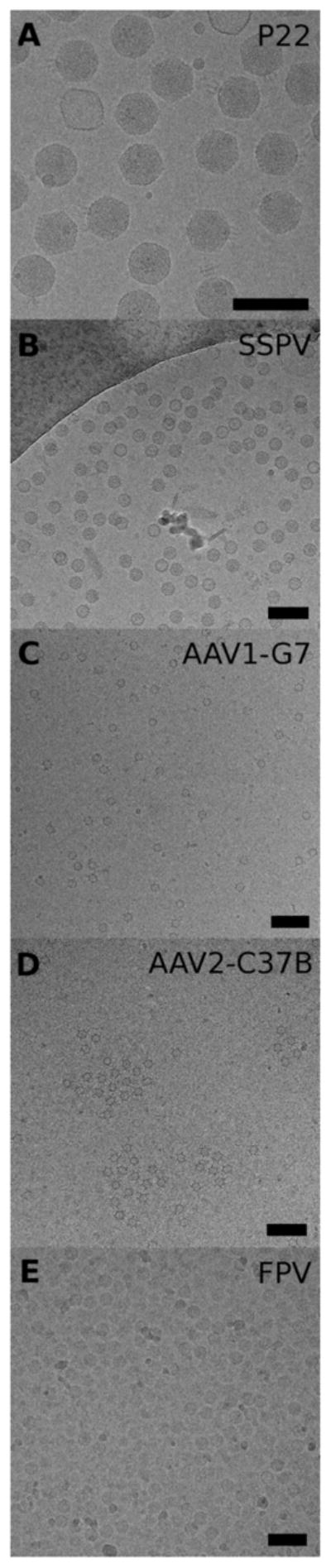
Data sets used for the benchmark tests. A representative micrograph is shown for each data set (bar = 100 nm).

Figure 5.

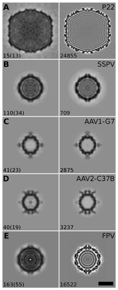
Equatorial density sections of reconstructions. For each data set, a comparison is shown between a 3D reconstruction determined from the particles in one micrograph and the 3D reconstruction from all the particles available. The relative contrast of the reconstructions is the same as that used for Figure 3 (i.e. high density features appear darker than the surrounding background). Bar, 20 nm. Left column: central sections of the 3D reconstructions obtained from selected micrographs by AutoRTM. The number of particle images extracted automatically from each selected micrograph and how many of those agree with the particles selected manually by the user (in parenthesis) are noted at the bottom left of each panel. Right column: central sections of 3D reconstructions obtained from entire data sets of micrographs as originally processed by experienced users. The number of particle images used to compute each reconstruction is given at the bottom left of each panel.

Except for the SSPV data set, which consisted of 17 micrographs, the other four data sets comprised at least one hundred micrographs, thus making these results statistically significant. It is important to note that the micrographs were included in the analysis without any a priori screening.

4.2 Computational time

The determination of a 3D reconstruction from a set of particle images, starting from a single raw micrograph, requires several processing steps, as previously described, each one contributing to the total computation time. We evaluated the timing on our cluster for all the micrographs available in each of the data sets chosen (Table 2), using a total of 20 processors in parallel. The time changes with each data set, ranging from an average of 44 seconds for the AAV-Fab complexes to more than 2 minutes for phage P22. These timings were obtained using micrographs that were binned before processing. For example, the P22 micrographs were binned to a pixel size of 5 Å from the original value of 1.0 Å: we observed that by reducing the binning to 4 Å, the average compute time per micrograph increased dramatically (by 66%, from 149 s to 248 s). In our approach, the most intensive computational step is the determination of a 3D reconstruction from the extracted particle images, which is performed using the RMC method. Even by running in parallel the iterative refinement of the ten (by default) random models initially generated, the computation consumes 80% or more of the total time, depending on the data set. The only other step that requires any significant computation is the defocus estimation, which in our tests was obtained within 6 seconds. Though the current algorithm for particle picking requires less than one second, it is nonetheless executed in parallel with the defocus estimation, since the two processes are completely independent. This mode of operation also allows us, in the future, to evaluate alternative particle-picking algorithms that may be more accurate (see below), without impacting significantly the current performance of the system.

Table 2.

Computational time required to reconstruct a 3D structure from one micrograph

	P22	SSPV	AAV1-G7	AAV2-C37B	FPV
10-RMC time (s)a,b	78 ± 3	57 ± 5	24 ± 2	24 ± 3	59 ± 2
1-RMC time (s)a,c	39 ± 1	34 ± 3	17 ± 1	17 ± 1	39 ± 2

^aThe time (secs) is reported as the average ± standard deviation, and it includes all processing steps.

^bThe 10-RMC time is the time measured when ten RMCs, each one running on two processors and consisting of ten iterations of alignment and reconstruction, are distributed in parallel.

^cThe 1-RMC time is the time observed when only one RMC is run. The difference between the two timings arises as a consequence of competition for I/O resources when multiple processes access the same disk.

During testing, we observed that the system performance decreased as a function of the number of random models being computed simultaneously. This behavior was shown to depend on the concurrent writing out to the disk storage device of the reconstructed 3D density maps, one per iteration and per random model, through the network. To evaluate how network bandwidth affected performance, we repeated the tests by decreasing the number of RMCs to just one. This “1-model” timing result (Table 2) represents an ideal situation (i.e. minimum time) in which no I/O bottlenecks are encountered. The difference between the timings for the 1-model verses 10-model tests was highest for the largest particles (P22 data), where performance decreased two-fold, and it is less relevant for the smallest particles. In the latter instance, it is important to note that all the timings fall within one minute. Further improvements could be achieved by adopting alternative hardware configurations where the I/O over the network is either reduced, using local disks on each node to store the intermediate results, or optimized by employing parallel file systems. We also performed additional tests on a laptop computer equipped with an Intel Core 5 processor and 4 GB of memory, where the processing could take advantage of the direct access to the data on the local disk. In this test, which employed two cores for each RMC, but executing the ten computations in sequence rather than in parallel, the average timing measured for a subset of the full set of micrographs of AAV2-C37B was about one minute, which compares favorably to the 24 seconds measured on the cluster using five times more processor cores.

The number of particle images that are picked from a micrograph is expected to affect the time needed to obtain a reconstruction, since the orientation parameters are determined for each particle. However, there was no strong dependency between these two quantities (Figure 4). In our case a weak linear trend is evident just for the SSPV and AAV2-C37B data, which are the only data sets that exhibited large variations in the number of particles in each micrograph. Also, as previously mentioned, the size of the particles directly affects system performance. The timings measured from micrographs of P22 cluster separately from the other data sets, which are for particles that are more similar in diameter (Figure 4). As a result, it takes more time to process a micrograph containing 15 particles of P22 (diameter = 550 Å) than a micrograph of FPV (diameter = 320 Å), which contains almost ten times more particles.

Figure 4.

Dependency of computational time on number of particles picked from each micrograph. Plot of the time required to process each micrograph and calculate one random model (1-RMC time) against the number of particles automatically picked and used for each reconstruction. All times are rounded to the nearest second.

4.3 Reconstruction from one micrograph

One micrograph displays particles whose number varies with their concentration and size, and also depends on the field of view, which is determined by the magnification setting of the microscope. In the data sets used for our tests, this number ranged from a low of 2 (AAV1-G7) to a maximum of 98 (AAV2-C37B), as estimated from the particles picked manually by the users who had originally analyzed the data. From such low numbers of particles, it is unreasonable to expect that a high resolution reconstruction could be generated from the proposed processing scheme. Therefore, we set the target resolution to 28 Å, which is an arbitrary value determined by experience. At this resolution level a 3D reconstruction still conveys useful information about the structure of particles in the sample (Figure 5). In the case of the two AAV-Fab complexes, the reconstructions obtained from single micrographs, with about 40 particles selected, already revealed that the two antibodies bind differently to the AAV capsids. In addition, close comparison of the density levels for capsid verses Fab features in the reconstructions makes it possible to estimate the stoichiometry of binding. The low resolution capsid structure of P22 was reconstructed from just 15 particle images, while more than one hundred were used in computing the SSPV and FPV reconstructions. It is noteworthy that for these two micrographs less than one third of the particle images used in the automatic processing overlapped with those selected by the experienced user. The remaining particles picked automatically were either false positives or they were identified by the user as ‘bad’ particles (e.g. malformed or damaged). Nevertheless, the RMC method proved robust enough to enhance the components that are well preserved and maintain a consistent structure in most particles, while any random components only serve to increase the noise level in the final model.

4.4 Success rate

The fidelity of the reconstruction is definitely one of the most relevant indicators of the performance of the system, but it is also the most difficult to assess in a rigorous and reliable manner. In most typical applications, when the RMC approach is used on a full data set to determine an initial reference model, up to 150 particles are selected from two or more micrographs among the ones with higher defocus. Using this approach it is usually possible to discriminate quite reliably, either visually or by other quantitative criteria, between correct and incorrect reconstructions. On the contrary, in the set of tests we describe here, each reconstructed density map is obtained from one micrograph with arbitrary defocus and usually contains much fewer than 150 particles (eg. as few as 10 in our tests with P22). More significantly, a subset of the particle images included in the iterative procedure is not of actual particles (false positives), owing to inaccuracies inherent in most automatic picking algorithms. Consequently, the maps determined from individual micrographs by the RMC approach are necessarily restricted in resolution, and this renders the distinction between correct and incorrect reconstructions as more elusive. We tested several metrics, including the variance of the map and the correlation coefficient between the map and a high-resolution reference, but none of these led to a desired bimodal distribution in which two populations could be separated by thresholding.

Eventually we classified all the reconstructed 3D density maps manually, by inspecting the central sections of each one. For comparison, and in an attempt to reduce bias in the selection process, we also implemented a semi-automatic classification procedure that grouped the maps into 40 clusters that were then inspected and judged visually (see §3.2.3). In this case, all members of a given cluster were classified as either correct or not, depending on how close the cluster average resembled the high-resolution reconstruction obtained from the entire data set of particle images. In this way, for each data set we reduced the visual analysis and the decision process by 250-fold (from ~10,000 to ~40 images). However, this approach did not prove to be completely accurate, since we observed that several clusters contained a mixed population of reconstructions, with obviously incorrect ones being assigned to a cluster that contained a majority of correct models, and vice versa.

Once the reconstructions were scored as correct or incorrect according to their fidelity to the target reconstruction, we measured the success rate of the method as the percentage of micrographs that yielded a correct map (Table 3). In this regard, the FPV data set performed the worst, with the procedure being successful with 62% of the micrographs. This result correlates with the overall poor quality of the micrographs, as observed earlier, which is the worst among the five sets analyzed and reported here. The success rate exceeded 70% in the other four data sets, and for SSPV and P22 it was better than 90%. We also estimated the average number of correct models generated by the RMC approach, computed for just those micrographs that successfully resulted in a reconstruction (Table 3). Since the RMC method is always successful as long as one out of the ten models is correct, and it is able to discriminate it as such, this number is not a strict indicator of the ability to get a correct reconstruction. Rather, it gives a quantitative hint of how easy is to get a correct map from the given particles. When comparing the success rate with the number of correct models as defined above (Table 3), we saw no strict dependency. In fact, previous studies (Yan et al., 2007a) as well as extensive experience with a wide range of different data sets have shown that the probability of producing a correct 3D reconstruction starting from a random model depends primarily on the defocus level of the micrograph and on the coarseness of features on the surface of the particles. In this context the situation is more complicated because the accuracy of the picking algorithm is an additional factor that affects success and must be considered (see §4.6).

Table 3.

Accuracy of automated workflow

	P22	SSPV	AAV1-G7	AAV2-C37B	FPV
Success rate (%)a,c	92 (82)	94 (94)	63 (71)	85 (81)	62 (51)
Correct models out of 10b,c	4±2 (4±2)	8±1 (8±1)	3±2 (3±2)	5±2 (5±2)	4±2 (4±2)

^aSuccess rate defines the frequency at which the approach obtained a correct 3D reconstruction.

^bThe number of correct random models, out of the ten computations launched for each micrograph, are reported in the second row as the average ± standard deviation.

^cThe success of a complete RMC run, including preprocessing steps, was determined after manually classifying all the reconstructions generated. Results obtained by classifying the reconstructions by Principal Component Analysis and k-means clustering are reported in parentheses.

Most of the results presented here were obtained by calculating ten random models and performing ten iterations of alignment for each of them. These are the same default settings adopted for the RMC approach, when used for determining an initial template from selected micrographs recorded at high defocus and containing a net total of at least 150 particles. Based on previous experience, these parameters generally guarantee convergence to a reliable template for almost all the data sets analyzed in their entirety. Since the approach here is implemented under quite different and more stringent conditions, we tested how the success rate correlates with each of these two parameters. The correctness of the reconstructions was assessed both manually (Figure 6) and on the basis of a semi-automatic classification procedure (Figure S1). When the number of random models computed in parallel is fixed at the default setting of ten (Figure 6A), the success rate increases rapidly with increasing iterations of alignment, though the rate of convergence differs for each data set. For example, the SSPV and AAV2-C37B data sets converge rapidly in three or five iterations, respectively, to a success rate that does not change significantly with subsequent iterations. Conversely, the P22 and AAV1-G7 data sets don’t seem to reach an asymptotic value, and would likely benefit from additional iterations. Hence, the choice of ten iterations as a default represents a compromise between computational speed and accuracy.

Figure 6.

Analysis of factors that affect success rate. (A, B) Success rate plotted against the number of iterations used to process ten initial random models. (C, D) Success rate plotted against the number of RMCs executed through ten iterations. In (A) and (C) the initial random models were generated from particle images picked automatically. In (B) and (D) the random models were generated from particle images identified manually in the micrographs.

When considering dependency of success rate on the number of random models, with each one processed through ten iterations (Figure 6C), for all data sets but FPV and AAV1-G7, two random models are enough to achieve a success rate above 50%. Furthermore, use of eight random models already achieves a success rate that is very close (within 4%) to that achieved with ten models. Hence, we consider the default choice of running ten models as being a conservative one. In our configuration, where the random models are processed in parallel, reducing the number of random models reduces the number of processors needed, but doesn’t necessarily decrease the total computational cost.

We also tested if the number of particles in a micrograph affects the probability of obtaining a correct reconstruction, but no obvious trend could be detected (data not shown). For just the FPV data set, those micrographs that contained fewer particle images than the average did yield a significantly lower fraction of valid 3D reconstructions. In general we observed that the quality of the particles picked, rather than their number, was a more significant determinant of success rate. In fact the rate increases dramatically when the particles are carefully selected by the user, as shown by the corresponding dependency analysis on number of iterations (Figure 6B) and number of models (Figure 6D) (see §4.6).

4.5 Performance of Preprocessing Steps

The task of the RMC step is to derive the origin and orientation parameters for a set of 2D images of particles, and to use the parameters to correctly combine the images, after correction for the microscope CTF, into a 3D reconstruction. Since the process is calibrated to generate low resolution reconstructions, the accuracy of the defocus estimate is not expected to be critical for the success of the approach. Conversely, we did expect that the accuracy of the particle-picking algorithms would affect the success rate of the procedure. To test these two hypotheses, we measured the inaccuracies in the algorithm used to estimate the defocus level and to pick particles with the previous results obtained manually by the experienced users as a ‘gold standard’ reference.

4.5.1 Defocus estimate

We estimated the CTF of each micrograph using a customized version of CTFFIND3 (Mindell and Grigorieff, 2003), which was further optimized by us only to enhance performance. The estimate was performed on micrographs binned to 2048 × 2048 pixels, independent of pixel size. The defocus search range was set to between 0.8 and 4 μm underfocus by default. We found that these settings were robust in most situations, and the program could still determine a defocus value that fell outside the default range. However, for the SSPV data set, which involved the recording of many micrographs at high defocus values (up to 8 μm), we reset the range to be between 3 and 7 μm. The requirement to change the default range to accommodate particular conditions of microscopy is not generally desirable in an automated workflow like this one, and an alternative approach might be to re-hardwire the default range between 0.8 and 7 μm to encompass a more diverse set of experimental situations. However, the cost of this strategy would entail an approximate doubling of the time required for estimating the defocus, and this would necessarily extend the total compute time. Therefore, we currently allow the microscopist to override the default settings if necessary, rather than imposing a computational burden on any particular data acquisition.

We measured the defocus error for each micrograph, defined as the difference between the estimate made by the user and that made by the program (Figure 7). Except for the SSPV data set, where the measured errors centered around zero, the program tended to overestimate the defocus level compared to that made by the experienced user. These results, however, are inconclusive, since we have no reliable means to assure that the user’s estimate of defocus was completely accurate. However, data sets were not all processed by the same user or using the same set of programs, which rules out a systematic bias on the user side. Overall, it seems more plausible that the program is sensitive to the quality of the micrographs and to the fraction of the field of view occupied by particles, which translates to the amount of signal available for the estimate. Accordingly, the largest variations of defocus errors were observed for the AAV1-G7 and AAV2-C37B data sets, which are also the ones with the smallest size and least number of particles. The other three data sets exhibited errors of less than 5% for most of the micrographs (Table 4). Furthermore, in the AAV2-C37B data set the defocus error was higher for the micrographs acquired at lower nominal defocus.

Figure 7.

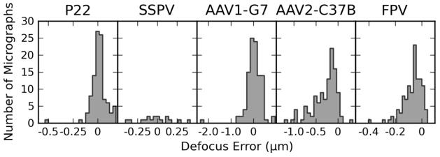
Defocus error analysis. Histogram plot of defocus error estimated for each data set. The error is defined as the difference between the average defocus value estimated by an experienced user and the average defocus value obtained using the AutoRTM program. Note that the scale of the abscissa is different for each plot.

Table 4.

Performance of preprocessing algorithms

	P22	SSPV	AAV1-G7	AAV2-C37B	FPV
Defocus error (μm)a,b	0.01 ± 0.08	−0.02 ± 0.20	0.02 ± 0.36	−0.29 ± 0.27	−0.07 ± 0.07
Defocus error (%)a,b	0.7 ± 5	−1.1 ± 6	−0.4 ± 16	−13.4 ± 15	−4.1 ± 5
Recall (%)a,c	94 ± 7	95 ± 5	69 ± 16	65 ± 15	74 ± 14
Precision (%)a,c	84 ± 9	33 ± 7	38 ± 19	36 ± 15	23 ± 5

^aAll measures are reported as an average ± standard deviation.

^bDefocus error is the difference between the average defocus value estimated by the user and the average defocus derived from the automated calculation, and it is reported in absolute (first row) and relative values (second row).

^cRecall and precision measure the accuracy of the picking algorithm.

4.5.2 Particle picking

Location and extraction of particles from each micrograph is performed using a multi-step algorithm that combines the Crosspoint Method, a heuristic approach, with correlation refinement (Boier Martin et al., 1997). The routines are implemented in the program RobEM, a visualization and analysis tool that is a component of the Auto3DEM software (Yan et al., 2007b). In this case the program is launched in batch mode, without graphical interface. The current implementation has been marginally modified with respect to the original described in (Boier Martin et al., 1997), mainly to improve its performance and to make it more robust under a larger range of image quality conditions. In particular, the implementation has been calibrated using several micrographs of different quality, with the goal to prioritize minimizing the miss rate as opposed to trying to minimize the number of false hits. A general description of the current algorithm, decomposed in its processing steps, is given in Appendix A. The program requires one input parameter from the user, which is an approximate radius of the targeted particles in the micrograph. This parameter is used at the initial step of the picking process to determine the level of image compression and to set the scan radius for the Crosspoint Method. Notably, this is the only parameter that needs to be given to initiate the automated analysis. Particle picking and extraction, which took one second or less in our tests, are performed simultaneously with CTF estimation, in parallel.

We evaluated the performance of the picking algorithm by measuring the precision and the recall for each micrograph (Figure 8). Precision is defined as the fraction of picked ‘particles’ that are true particles, whereas recall is the fraction of all true particles in the micrograph that are picked (Langlois and Frank, 2011). The complements of these two functions correspond to the fraction of false positives and to the miss rate, respectively. To be completely accurate, these measures require knowledge of the total number of genuine particles in each micrograph, whereas for experimental micrographs only the number of particles selected by the user is available. The two numbers can be different because an experienced user usually only selects particles that show good properties according to criteria developed by personal experience. Therefore, a comparison of results obtained by automatic picking with those obtained manually by one user may yield some biased measure of the accuracy of the algorithm. In our tests, the P22 data set is the only one in which almost all the particles in the micrographs, except for a few that are empty, were picked by the user. Also, the size and the concentration of the P22 particles make those data an ideal target for automatic picking procedures. The other data sets presented more challenges, as previously described. The recall (i.e. the agreement between algorithm and user) exceeded 90% for the P22 and SSPV data sets, where the particles are relatively easy to recognize owing to their size or high contrast, respectively. For particles that are empty and relatively small (AAV-Fab complexes), or are embedded in higher levels of noise (FPV), the agreement dropped to ~70%. Concerning the false positives, the algorithm only achieved high precision (~85%) with the P22 data set. In the other test cases, the value decreased to less than 40%, meaning that more than half of the picked particles were either false positives or particles that were not picked by the user. We inspected individual micrographs of SSPV and FPV, which gave the lowest precision scores, to ascertain the cause of such low performance. For SSPV there is a mixed population of genome-empty verses genome-full capsids. The experienced user only picked genome-full capsids, but the picking algorithm failed to discriminate the two subsets. For FPV, the edges of particles are not always well defined in a particular micrograph owing to the large thickness of the vitrified specimen. In such instances, the user only selected particles exhibiting high contrast, whereas the program also selected particles that were more embedded in the background noise. Except for P22 and a small fraction of the AAV-Fab images, for each micrograph we found that the recall always exceeded the precision.

Figure 8.

Particle detection analysis. Left column: plot of precision against recall for all the micrographs processed. A red ellipse is drawn for each data set centered at the average value for each measure, with semi-axes equal to the standard deviation. Right column: plots of precision against the average defocus as estimated by an experienced user. Note that the scale of the defocus axis is different for each plot.

We also analyzed how defocus affects the accuracy of the picking algorithm, and observed that there is only a weak dependency (Figure 8). In the AAV-Fab and FPV data sets, the precision tended to be higher for micrographs acquired at higher defocus, but this behavior was not evident in the other data sets. We did not observe any dependency between recall and defocus (data not shown).

4.6 Particle picking affects reconstruction accuracy

The number and the quality of the particles extracted from a micrograph are expected to affect whether the RMC method can produce a reliable 3D reconstruction. Depending on the data set, the algorithm currently used to automatically pick particles can include numerous false positives, sometimes exceeding 50% of the total number. To analyze how precision affects success rate, we repeated the entire analysis with just the sets of particles picked manually by experienced users (Figure 6B, D; Table 5). A comparison with respect to the complete automatic approach (Figure 6A, C and Table 3) shows that the number of correct reconstructions, out of the ten generated for each micrograph, tends to increase when supposedly there are no false positives (i.e. the user is assumed to be 100% accurate). The largest improvement was seen for the FPV data set, where the number of correct reconstructions generated almost doubles, on average, from 4 out of 10 to 7 out of 10. In this example, the precision of the automated procedure was only 23%, and the success rate increased from 62 to 99% for particles that were selected manually. However, except for the FPV data, a higher precision value does not necessarily correlate with a higher success rate. For the SSPV data set, where the precision was ~33%, the success rate did not change when using particle images selected by the user, and the difference improved only by 10% for the AAV2-C37B data set, where the precision was ~38%. Conversely, the particles selected manually from the AAV1-G7 micrographs did show an improvement of the success rate from 63% to 82% even though the precision of this set was also 38%.

Table 5.

Accuracy of the system for particles picked manually

	P22	SSPV	AAV1-G7	AAV2-C37B	FPV
Success rate (%)a,b	87 (87)	94 (94)	82 (82)	95 (94)	99 (96)
Correct models out of 10a,b,c	4±2 (4±2)	9±1 (9±1)	4±2 (4±2)	5±2 (5±2)	7±2 (7±2)

^aSuccess rate and number of correct random models per micrograph were calculated after repeating the experiments reported in Table 3 but without determining automatically the positions of particles in the micrographs, and, instead, using the coordinates determined previously by an expert user. Definitions of the measures are given in Table 3.

^bResults obtained by classifying the reconstructions by Principal Component Analysis and k-means clustering are reported in parentheses.

^cThe number of correct random models is reported as average ± standard deviation.

Conclusions

We have developed an integrated approach that can provide 3D structural information from samples of icosahedral particles in rapid and automated fashion. The approach is implemented in the program AutoRTM, which provides visual feedback to the microscopist of the results of the analysis on the particles in a single micrograph generally within a minute from its acquisition. By inputting only minimal information to the program (approximate particle radius and the name of a directory where newly acquired data are stored), the microscopist can receive valuable preliminary information about the structure of the particle being studied. For samples that present specific challenges, additional parameters, like the defocus range or the size of the boxed particles, can be controlled as advanced settings. AutoRTM augments the structural information available at the microscope, and it can be particularly useful when screening new samples targeted for acquisition of large data sets. In a future release the program will also permit data from more than one micrograph to be combined to yield a better resolved map that would be suitable as an initial template for the single particle analysis. This feature would also facilitate the screening of samples whose concentration is too low and only yields a few particles per micrograph. The advantages of the proposed approach extend beyond a simple assessment of sample quality. For example, the AAV-Fab data sets already illustrate one potential application. When samples are being prepared for the purpose of studying how monoclonal antibodies bind to a virus capsid, it is important to determine the extent to which the binding sites are saturated, as well as verifying if steric hindrance occurs as a result of alternative modes of binding. Such information can help determine if a sample is suitable for large scale data acquisition, and if the binding epitopes can be mapped at a sufficient level of detail. The results of our present analysis show that the 3D reconstruction obtained from the particle images contained in just one micrograph, when correct, already provide a reliable low resolution picture of the virus-antibody binding properties that surpasses what could be extracted simply from visual inspection or 2D analysis of the raw micrograph.

AutoRTM generates a new 3D reconstruction from each micrograph acquired. This approach is a useful means to assess the quality of each image separately, but it is not sufficiently robust to guarantee a successful result. Among the factors that affect the outcome of the RMC, we observed that the level of defocus used to record the micrograph and the number of particles present in the field of view only play a small role. This contrasts with our past experience in using the RMC method to determine an initial model, when higher defocus and a larger number of particles would increase the chance of obtaining an accurate ab initio reconstruction. Despite recent improvements to the RMC method that have made these requirements less stringent (Cardone et al, in preparation), it is relevant to note that previous results were obtained with particle images from particles picked manually by an expert user, usually from more than one micrograph. To the contrary, our new approach picks particles automatically, and the accuracy of the picking algorithm poses the major limiting factor in achieving success rates > 80%. Therefore, we are investigating the use of alternative, unsupervised picking algorithms, which satisfy the requirement of being more accurate within a time frame of a few seconds. Given the current setup, our results demonstrate that the microscopist can expect to obtain a reliable estimate of the 3D structural properties of a particle after acquiring two images at the microscope, and a third image ought to resolve any potential remaining doubt. However, we consider such estimates of system performance to be conservative, and in practice we expect that the approach should do better. In fact, the micrographs used to test the approach encompass a wider range of acquisition conditions compared to those usually adopted during a preliminary analysis of a sample. For example, it is common practice with most new samples to record an initial set of images at higher defocus compared to what is used to acquire a complete data set. As was demonstrated for the SSPV data set, where the range of defocus is shifted towards higher values, having a few high defocus, high contrast images definitely helps the automated system pick particles more accurately, and this does increase the success rate of the RMC.

Our approach has been designed to work on computing clusters, using parallel libraries that facilitate communication among processors on different nodes. The computational requirements here are relatively modest, and in our experiments we were able to satisfy the constraint of completing the analysis of one micrograph within a minute or so, by using up to 20 processors in parallel to handle the most intensive computational step (i.e. the RMC). However, recent technological advancements have enabled similar computing resources to be bundled in a single node or even into a desktop system. Hence, our goal is to expand the capabilities of the current system to exploit simple, multi-core systems.

Having rapid, real-time access to 3D structural information on a sample while it is in the microscope will accelerate the screening phase that precedes the launch of an acquisition campaign aimed at generating a high resolution model. In addition, this type of analysis provides a low resolution 3D structural model that can be used as an initial template for the data set to be acquired. In this way, processing of the data can start immediately after the first images are acquired, and reconstructions at successively higher and higher resolutions can be provided in real-time as more images are recorded.

Supplementary Material

01. Supplemental Figure 1.

Analysis of factors that affect the success rate, as determined by semi-automatic classification. This analysis is similar to that shown in Figure 3, except the validity of each reconstruction is not determined by individual inspection, but by clustering the reconstructions automatically into 40 groups, and determining the validity of each average. The assignment given to each cluster average was reflected to all of its members.

Appendix. Description of picking algorithm

The algorithm used to locate particles in a micrograph is based on the Crosspoint method (Boier Martin et al., 1997). Here we only outline the complete algorithm, mainly to highlight changes that have been implemented with respect to its original description. Here, the algorithm is depicted as a sequence of computational steps, with those that have been optimized labeled with a single asterisk (*) and those that have been added to the process labeled with a double asterisk (**). Additional details about individual steps can be found in the cited reference. The only inputs to the algorithm are the digitized micrograph and the particle radius, in pixels. The relative contrast in the micrographs is consistent with images from unstained, vitrified samples: black pixels (i.e. lowest intensity values) correspond to highest specimen mass thickness, and white pixels (i.e. highest intensity values) correspond to regions where the specimen mass thickness is lowest.

• 1Remove outlier pixels. Pixel values that fall farther than 10 times the standard deviation of all values within the entire micrograph are truncated.
• *2Compress micrograph. Image size is reduced by binning, by a factor that yields a particle radius of about 20 pixels. An exact copy is stored in a separate buffer, for later use (see steps 11 and 12).
• 3Enhance image by histogram equalization. Pixel values are equalized to be evenly distributed in the range between 0 and 127.
• *4Further enhance image by filtering. Each pixel value is replaced with the average from all neighboring pixels lying within a radial distance equal to one third of the particle radius.
• 5Enhance contrast. Reset the range of pixel values back to from 0 to 127.
• 6Binarize image (marking). Mark pixels that could be inside a particle using a double scan procedure. Pairs of pixels at distance equal to the particle radius are compared, and the pixel with lowest value is marked if their difference exceeds 2.5 gray levels. The result is a binary image.
• *7Separate clusters of neighboring particles by morphological processing. Apply two iterations of thinning to the binarized image, followed by one iteration of dilation.
• 8Identify particles by clustering. Find connected components in the image using the stack algorithm. Each cluster of connected pixels is identified as a putative particle.
• 9Filter particles by cluster size. Impose the following constraints on the clusters obtained at Step 8:
• 9aThe number of pixels in a cluster must be between 60% and 200% of the number of pixels contained in a circle of radius equal to that of the particle.
• 9bThe linear size of the maximum bounding box of the cluster can not exceed twice the particle diameter.
• *9cCalculate a score for each cluster, defined as the difference between the pixel average within the particle radius from the cluster center of mass and the pixel average in a shell just outside the radius, with thickness equal to 0.2 times the radius. The cluster is rejected, i.e. it is not identified as a particle, if the score is less than 2.5 (gray levels).
• **10Prune outliers with high scores. The goal of this step is to detect “contaminants” that we define here as exhibiting high contrast and being similar in size to the desired particle. Such contaminants are recognized as particles by the algorithm, and usually are assigned an excessively high score, as defined in 9c. The score is used to generate a histogram with the number of bins set equal to half the number of clusters. The histogram is then filtered using a moving average window with size equal to 1/10 of the full range. Subsequent analysis is limited to just the upper tail of the histogram (i.e. highest scores), and all particles in a bin that is smaller than the size of the moving window are rejected. The procedure is repeated until no particles are discarded.
• *11Screen particles by average density. Using the unprocessed binned micrograph obtained at Step 2, calculate the average density within the particle radius from the center of mass of each remaining cluster, and discard any cluster whose average exceeds three times the standard deviation of all the averages.
• 12Refine particle centers. A model particle projection is generated from the average of all the remaining particles, and the center of each particle is refined by maximizing the normalized cross-correlation between the particle and the model.

References

- Adiga U, Baxter WT, Hall RJ, Rockel B, Rath BK, Frank J, Glaeser R. Particle picking by segmentation: A comparative study with SPIDER-based manual particle picking. J Struct Biol. 2005;152:211–220. doi: 10.1016/j.jsb.2005.09.007. [DOI] [PubMed] [Google Scholar]
- Baker TS, Cheng RH. A model-based approach for determining orientations of biological macromolecules imaged by cryoelectron microscopy. J Struct Biol. 1996;116:120–130. doi: 10.1006/jsbi.1996.0020. [DOI] [PubMed] [Google Scholar]
- Bammes BE, Rochat RH, Jakana J, Chen DH, Chiu W. Direct electron detection yields cryo-EM reconstructions at resolutions beyond 3/4 Nyquist frequency. J Struct Biol. 2012;177:589–601. doi: 10.1016/j.jsb.2012.01.008. [DOI] [PMC free article] [PubMed] [Google Scholar]
- Boier Martin IM, Marinescu DC, Lynch RE, Baker TS. Identification of spherical virus particles in digitized images of entire electron micrographs. J Struct Biol. 1997;120:146–157. doi: 10.1006/jsbi.1997.3901. [DOI] [PubMed] [Google Scholar]
- Frank J. Three-Dimensional Electron Microscopy of Macromolecular Assemblies. Oxford U. Press; 2006. [Google Scholar]
- Gurda BL, DiMattia MA, Miller EB, Bennett A, McKenna R, Weichert WS, Nelson CD, Chen W, Muzyczka N, Olson NH, Sinkovits RS, Chiorini JA, Zolotutkhin S, Kozyreva OG, Samulski RJ, Baker TS, Parrish CR, Agbandje-McKenna M. Capsid Antibodies to Different Adeno-Associated Virus Serotypes Bind Common Regions. J Virol. 2013 doi: 10.1128/JVI.00622-13. accepted. [DOI] [PMC free article] [PubMed] [Google Scholar]
- Heymann JB, Belnap DM. Bsoft: image processing and molecular modeling for electron microscopy. J Struct Biol. 2007;157:3–18. doi: 10.1016/j.jsb.2006.06.006. [DOI] [PubMed] [Google Scholar]
- Hunter JD. Matplotlib: A 2D Graphics Environment. Comput Sci Eng. 2007;9:90–95. [Google Scholar]
- Jensen GJ. Preface. In: Jensen Grant J., editor. Methods in Enzymology. Academic Press; 2010. pp. xv–xvi. [Google Scholar]
- Jones S, Bruno G, McIntire T. Rocks clusters. Proceedings of the 2006 ACM/IEEE Conference on Supercomputing, SC’06; New York, NY, USA: ACM; 2006. [Google Scholar]
- Korinek A, Beck F, Baumeister W, Nickell S, Plitzko JM. Computer controlled cryo-electron microscopy--TOM2 a software package for high-throughput applications. J Struct Biol. 2011;175:394–405. doi: 10.1016/j.jsb.2011.06.003. [DOI] [PubMed] [Google Scholar]
- Lander GC, Tang L, Casjens SR, Gilcrease EB, Prevelige P, Poliakov A, Potter CS, Carragher B, Johnson JE. The Structure of an Infectious P22 Virion Shows the Signal for Headful DNA Packaging. Science. 2006;312:1791–1795. doi: 10.1126/science.1127981. [DOI] [PubMed] [Google Scholar]
- Langlois R, Frank J. A clarification of the terms used in comparing semi-automated particle selection algorithms in cryo-EM. J Struct Biol. 2011;175:348–352. doi: 10.1016/j.jsb.2011.03.009. [DOI] [PMC free article] [PubMed] [Google Scholar]
- MacQueen J. Some methods for classification and analysis of multivariate observations. Proc. Fifth Berkeley Sympos. Math. Statist. and Probability; Berkeley, Calif. 1965/66; Berkeley, Calif: Univ. California Press; 1967. pp. 281–297. Vol. I: Statistics. [Google Scholar]
- Mallick SP, Carragher B, Potter CS, Kriegman DJ. ACE: automated CTF estimation. Ultramicroscopy. 2005;104:8–29. doi: 10.1016/j.ultramic.2005.02.004. [DOI] [PubMed] [Google Scholar]
- Mindell JA, Grigorieff N. Accurate determination of local defocus and specimen tilt in electron microscopy. J Struct Biol. 2003;142:334–347. doi: 10.1016/s1047-8477(03)00069-8. [DOI] [PubMed] [Google Scholar]
- Ogura T, Sato C. Auto-accumulation method using simulated annealing enables fully automatic particle pickup completely free from a matching template or learning data. J Struct Biol. 2004;146:344–358. doi: 10.1016/j.jsb.2004.01.007. [DOI] [PubMed] [Google Scholar]
- Oliphant TE. Python for Scientific Computing. Comput Sci Eng. 2007;9:10–20. [Google Scholar]
- Pearson K. On lines and planes of closest fit to systems of points in space. Philos Mag. 1901;2:559–572. [Google Scholar]
- Shi J, Williams DR, Stewart PL. A Script-Assisted Microscopy (SAM) package to improve data acquisition rates on FEI Tecnai electron microscopes equipped with Gatan CCD cameras. J Struct Biol. 2008;164:166–169. doi: 10.1016/j.jsb.2008.05.011. [DOI] [PMC free article] [PubMed] [Google Scholar]
- Suloway C, Pulokas J, Fellmann D, Cheng A, Guerra F, Quispe J, Stagg S, Potter CS, Carragher B. Automated molecular microscopy: the new Leginon system. J Struct Biol. 2005;151:41–60. doi: 10.1016/j.jsb.2005.03.010. [DOI] [PubMed] [Google Scholar]
- Tang J, Lander GC, Olia AS, Olia A, Li R, Casjens S, Prevelige P, Jr, Cingolani G, Baker TS, Johnson JE. Peering down the barrel of a bacteriophage portal: the genome packaging and release valve in P22. Structure. 2011;19:496–502. doi: 10.1016/j.str.2011.02.010. [DOI] [PMC free article] [PubMed] [Google Scholar]
- Tang J, Ochoa WF, Li H, Havens WM, Nibert ML, Ghabrial SA, Baker TS. Structure of Fusarium poae virus 1 shows conserved and variable elements of partitivirus capsids and evolutionary relationships to picobirnavirus. J Struct Biol. 2010;172:363–371. doi: 10.1016/j.jsb.2010.06.022. [DOI] [PMC free article] [PubMed] [Google Scholar]
- Vargas J, Otón J, Marabini R, Jonic S, de la Rosa-Trevín JM, Carazo JM, Sorzano COS. FASTDEF: fast defocus and astigmatism estimation for high-throughput transmission electron microscopy. J Struct Biol. 2013;181:136–148. doi: 10.1016/j.jsb.2012.12.006. [DOI] [PubMed] [Google Scholar]
- Voss NR, Yoshioka CK, Radermacher M, Potter CS, Carragher B. DoG Picker and TiltPicker: Software tools to facilitate particle selection in single particle electron microscopy. J Struct Biol. 2009;166:205–213. doi: 10.1016/j.jsb.2009.01.004. [DOI] [PMC free article] [PubMed] [Google Scholar]
- Yan X, Dryden KA, Tang J, Baker TS. Ab initio random model method facilitates 3D reconstruction of icosahedral particles. J Struct Biol. 2007a;157:211–225. doi: 10.1016/j.jsb.2006.07.013. [DOI] [PMC free article] [PubMed] [Google Scholar]
- Yan X, Sinkovits RS, Baker TS. AUTO3DEM--an automated and high throughput program for image reconstruction of icosahedral particles. J Struct Biol. 2007b;157:73–82. doi: 10.1016/j.jsb.2006.08.007. [DOI] [PMC free article] [PubMed] [Google Scholar]
- Yu X, Ge P, Jiang J, Atanasov I, Zhou ZH. Atomic Model of CPV Reveals the Mechanism Used by This Single-Shelled Virus to Economically Carry Out Functions Conserved in Multishelled Reoviruses. Structure. 2011;19:652–661. doi: 10.1016/j.str.2011.03.003. [DOI] [PMC free article] [PubMed] [Google Scholar]
- Zheng SQ, Keszthelyi B, Branlund E, Lyle JM, Braunfeld MB, Sedat JW, Agard DA. UCSF tomography: an integrated software suite for real-time electron microscopic tomographic data collection, alignment, and reconstruction. J Struct Biol. 2007;157:138–147. doi: 10.1016/j.jsb.2006.06.005. [DOI] [PubMed] [Google Scholar]
- Zhou ZH. Atomic resolution cryo electron microscopy of macromolecular complexes. Adv Protein Chem Struct Biol. 2011;82:1–35. doi: 10.1016/B978-0-12-386507-6.00001-4. [DOI] [PMC free article] [PubMed] [Google Scholar]
Associated Data
This section collects any data citations, data availability statements, or supplementary materials included in this article.
Supplementary Materials