Protein–protein alternative binding modes do not overlap

Abstract

Proteins often bind other proteins in more than one way. Thus alternative binding modes is an essential feature of protein interactions. Such binding modes may be detected by X-ray crystallography and thus reflected in Protein Data Bank. The alternative binding is often observed not for the protein itself but for its structural homolog. The results of this study based on the analysis of a comprehensive set of co-crystallized protein–protein complexes show that the alternative binding modes generally do not overlap, but are spatially separated. This effect is based on molecular recognition characteristics of the protein structures. The results are also in excellent agreement with the intermolecular energy funnel size estimates obtained previously by an independent methodology. The results provide an important insight into the principles of protein association, as well as potential guidelines for modeling of protein complexes and the design of protein interfaces.

Introduction

Structural characterization of protein–protein interactions is important for understanding molecular mechanisms in biology. Protein–protein complex formation can be viewed from either a physical perspective, as a path to the minimum of the free energy of the system, or from an empirical point of view, as a match between various phenomenological structural and physicochemical motifs (so called “recognition factors”). The structural characterization of the protein interactions inherently involves structural recognition factors responsible for the formation of the protein–protein complex.¹ It is well established that steric/geometric complementarity is at the heart of protein–protein recognition.^2–5 The binding sites for protein–protein interactions responsible for the intermolecular fit are large structural fragments with the recognition surface shape determined to a significant extent by the main-chain conformation.⁶ The binding sites of the larger protein in the complex are on average concave.⁷ However, more generally, the principal structural characteristic of the protein recognition is that the low resolution shape of a protein has functional importance⁸ and large structural motifs are responsible for the overall configuration of the protein–protein complex.^9,10

The existence of the large-scale structural recognition factors in protein association has to do with the funnel-like intermolecular energy landscape. The general slope of the energy landscape toward the native structure (“the funnel”) explains the kinetics of protein folding.¹¹ This concept is also necessary to explain the kinetics data on protein–protein association.^12,13 The existence of a funnel in protein–protein interactions is supported by multiple structural and physicochemical considerations, including the geometry (shape) of the proteins.^13,14 The characteristic funnel size is 6–8 Å interface root-mean-square deviation (RMSD).¹⁵ Because of the principal role of steric complementarity in protein–protein association, the geometric characteristics of the protein surfaces are responsible for the distribution of the intermolecular energy basins and the detection and size of the binding funnel.^15,16

Proteins often bind other proteins in more than one way. Thus alternative binding modes is an essential feature of protein interactions. The alternative binding modes may be detected by X-ray crystallography and thus reflected in Protein Data Bank (PDB). Such modes are often observed not for the protein itself but for its structural homolog. In this study, based on the analysis of a comprehensive set of co-crystallized protein–protein complexes, we show that the alternative binding modes generally are not overlapping, but are spatially separated. This effect is based on molecular recognition characteristics of the protein structures. The results are also in excellent agreement with the intermolecular energy funnel size estimates obtained previously by an independent methodology.¹⁵ The results provide an important insight into the principles of protein association,^5,17,18 as well as potential guidelines for modeling of protein complexes^1,19,20 and the design of protein interfaces.^21,22

Results and Discussion

The study is based on two sets of protein–protein complexes from PDB. The first, non-redundant representative set consists of 372 bound (co-crystallized) complexes that reflect typical protein–protein interactions in PDB. The second, much larger redundant set of 11,932 complexes represents the entire spectrum of protein–protein interactions in PDB, excluding only almost identical entries. All complexes in the large set are taken from the biological unit files, and thus are presumably biological.

The proteins from the small set (“targets”) were structurally aligned with the ones in the large set (“templates”), to detect the structural homologs of the targets. Then the complexes of the homologs were examined with relation to the complexes of the targets. For that purpose, the targets were spatially overlapped with their structural homologs in the templates complexes, and the distribution of the interface C^α RMSD (i-RMSD) values for such overlapped structures was analyzed. The study involved homologs in order to have proper statistics of the alternative binding modes. Comparison of the complexes generated by the spatial overlap, rather than a direct comparison of the complexes of the homologs, was used to calculate the RMSD (which can be calculated between different positions of the same molecule, but not between different molecules).

Figure 1 shows the distribution of i-RMSD values for all structures generated using all detected templates for the targets. The native-based distribution is sharply bimodal, with a very distinct minimum around 6–7 Å i-RMSD. All complexes in the distribution (both with small and large i-RMSD) are the overlapped structures that coincide with the experimentally determined, biological interactions of their homologs. Since they are not different from each other in that regard, the sharp minimum at 6–7 Å i-RMSD is so poignant. The minimum separates the binding modes that are similar to the X-ray target (smaller i-RMSD values) from the alternative binding modes (larger i-RMSD values). The gap between these modes indicates that they are generally well separated in space, with virtually no overlap.

Figure 1.

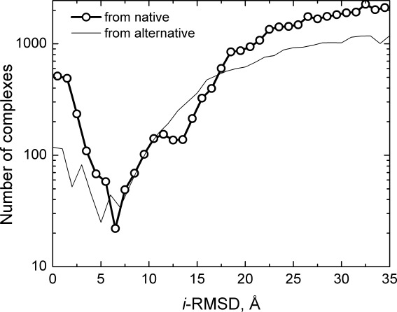
Distribution of protein–protein complexes generated by structural alignment with homologous templates. The i-RMSD is calculated relative to the native X-ray structure of the complex (thick line with circles), as well as to the generated structure with the largest i-RMSD from the native structure (thin line). The distinct minimum in the bimodal native-based distribution separates the main binding mode (smaller i-RMSD values) from the alternative binding modes (larger i-RMSD values). For comparison, the distribution from the alternative, most distant binding mode (the largest i-RMSD from the native structure) shows a similar to the native-based distribution pattern. A greater dispersion of values in this distribution corresponding to small i-RMSDs is likely caused by an overall smaller number of generated complexes (see text), and lower cluster occupancy at the putative alternative binding site, than at the native site.¹⁶ The qualitative similarity of the distributions, obtained from the different reference points, indicates similar separation of the binding modes.

For comparison, Figure 1 also shows the distribution of generated complexes relative to the generated structure with the largest i-RMSD from the native structure, showing a similar to the native-based distribution pattern. The reference complex (the one with the largest from the native i-RMSD) is not counted, similar to the absence of the native (X-ray) structure in the native-based distribution. The dispersion of values corresponding to small i-RMSDs is likely caused by (a) the smaller number of generated complexes (some reference-point template-based ligand modes are poorly positioned with regards to the receptor, making the determination of the interface ambiguous, compared to the one from a co-crystallized complex used in the native-based distribution), and (b) less cluster occupancy at the putative alternative binding site, than at the co-crystallized native site.¹⁶ The dip in the native-based distribution at 12–14 Å i-RMSD, is two times farther than the 6–7 Å i-RMSD separation between the native and the alternative modes, and thus may be the one separating the first and the second layers of the alternative binding modes (although this evidence is inconclusive). It disappears in the alternative-based distribution, likely due to the greater noise. In general, the qualitative similarity of the distributions in Figure 1, obtained from the different reference points, indicates similarity in the binding patterns (specifically, similar separation of the binding modes), as well as confirms the robustness of the analysis.

The binding modes separation effect reflects molecular recognition aspect based on the geometry of the protein structure, schematically shown in Figure 2. The gross (low-resolution) characteristics of protein shapes [e.g., concave interface as in Fig. 2(A) or convex interface as in Fig. 2(B)] are essential in protein recognition,⁹ requiring separation between the binding modes. Protein shapes are not isotropic—thus the binding modes scenario in Figure 2(C) is, in general, unlikely. Figure 3 illustrates this paradigm on a specific example of protein–protein configurations resulting from the structural alignment of homologous complexes. The binding pattern shows a clear separation of the binding modes.

Figure 2.

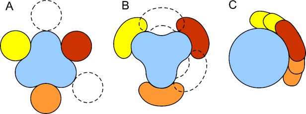
The concept of alternative binding modes in protein–protein interactions. The protein “receptor” is in blue and its binding protein partner (“ligand”) in the main binding mode (red) and the alternative binding modes (yellow and orange). The binding modes are based on the gross (low-resolution) geometric complementarity, in either concave (A) or convex (B) binding site on the receptor. In either case, the binding modes are separated in space, with the positions of ligand shown by dashed lines providing no shape complementarity for binding. Protein shapes are anisotropic, thus the binding scenario (C) where the alternative binding modes overlap is unlikely.

Figure 3.

An example of alternative binding modes. The distribution of the binding modes, based on the growth hormone/receptor complex 1axi,²³ was generated by structural alignment of the proteins from the complex to their co-crystallized structural homologs from a set of 11,932 protein–protein templates, as described in the text. The color scheme is the same as in Figure 2, with receptor in blue and ligand in the main binding mode (the same binding mode as the ligand co-crystallized with the receptor in the 1axi structure) in red, and the alternative binding modes in yellow and orange. The structural homologs (PDB code, chain 1 and 2) in the main binding mode are: 1a22BA, 1bp3BA, 1iarBA, 1pvhAB, 1eerCA, and 1eerBA; in the first alternative binding mode (yellow): 1wrdBA and 1yd8UH; and in the second alternative binding mode (orange): 1cd9DA and 1cd9BC. The binding pattern clearly shows the spatial separation of the binding modes.

Protein geometry is the determining factor of intermolecular energy landscapes.^13,14 Interestingly, from this perspective, the distribution in Figure 1 complements the results of the previous studies based on systematics sampling of the intermolecular energy landscapes by rigid-body template-free docking^13,16 that show several spatially separated funnel-like energy basins potentially corresponding to alternative binding modes. It also confirms the binding funnel size estimates, obtained by such sampling, in the 6–8 Å i-RMSD range.¹⁵ These numbers are in remarkable correspondence with the values in Figure 1, obtained by a completely unrelated approach—structural alignment of homologous complexes. The results indicate that the structures following the main binding mode (shown in red in Figs. 2 and 3) fall within the corresponding intermolecular energy funnel, while the structures in alternative binding modes (shown in yellow and orange in Figs. 2 and 3) are in other corresponding funnels.

These results point to an interesting and important aspect of molecular recognition, and provide an insight into the general principles of protein structure.

Methods

A representative set of 372 nonredundant (purged at 30% sequence identity) bound complexes (targets), where each component of the complex is a single-chain protein, was structurally aligned with protein–protein complexes from a set of templates, according to previously described protocol.²⁴ Both target and template complexes were extracted from our Dockground resource.^3,25 The X-ray structures resolution of the templates had to be < 3 Å, they had to be at least a dimeric biological unit, and the sequence identity between different complexes had to be <90%. The resulting set consisted of 11,932 complexes. Biological unit coordinates were obtained from http://ftp://ftp.wwpdb.org/pub/pdb/data/biounit.

Binding modes were generated by spatial rearrangement of separate 3D structures of the target monomers to overlap with a template complex by structural alignment. The alignment was performed by TM-align²⁶ for C^α atoms only. The C^α alignment reduces the effect of conformational changes upon binding, thus enabling proper overlap of the unbound and bound fragments. The alignment quality was assessed by TM-score²⁷ that has values in the 0–1 range. TM-score > 0.5 indicates statistically significant fold similarity (the average TM-score of a random structure match is 0.17).^26,27 The pairs of the structural alignments were ranked by the sum of the receptor and ligand TM-scores, and those with the smallest of the receptor and the ligand TM-scores > 0.4 were retained to generate complexes (the choice of 0.4 threshold stems from our previous study,²⁸ which determined the binding mode similarity at the TM-score > 0.4). Similar target-template pairs (TM-score > 0.9 and sequence identity > 95%) were excluded from consideration. Transformation matrices from the alignments were applied to the target proteins to generate the pool of complexes. The complexes were evaluated in terms of RMSD between interface C^α atoms of the native and the generated structures (i-RMSD).

References

- 1.Vakser IA. Low-resolution structural modeling of protein interactome. Curr Opin Struct Biol. 2013;23:198–205. doi: 10.1016/j.sbi.2012.12.003. [DOI] [PMC free article] [PubMed] [Google Scholar]
- 2.Keskin O, Tsai CJ, Wolfson H, Nussinov R. A new, structurally nonredundant, diverse data set of protein–protein interfaces and its implications. Protein Sci. 2004;13:1043–1055. doi: 10.1110/ps.03484604. [DOI] [PMC free article] [PubMed] [Google Scholar]
- 3.Douguet D, Chen HC, Tovchigrechko A, Vakser IA. DOCKGROUND resource for studying protein–protein interfaces. Bioinformatics. 2006;22:2612–2618. doi: 10.1093/bioinformatics/btl447. [DOI] [PubMed] [Google Scholar]
- 4.Katchalski-Katzir E, Shariv I, Eisenstein M, Friesem AA, Aflalo C, Vakser IA. Molecular surface recognition: determination of geometric fit between proteins and their ligands by correlation techniques. Proc Natl Acad Sci USA. 1992;89:2195–2199. doi: 10.1073/pnas.89.6.2195. [DOI] [PMC free article] [PubMed] [Google Scholar]
- 5.Janin J. Principles of protein–protein recognition from structure to thermodynamics. Biochimie. 1995;77:497–505. doi: 10.1016/0300-9084(96)88166-1. [DOI] [PubMed] [Google Scholar]
- 6.Vakser IA. Main-chain complementarity in protein–protein recognition. Protein Eng. 1996;9:741–744. doi: 10.1093/protein/9.9.741. [DOI] [PubMed] [Google Scholar]
- 7.Nicola G, Vakser IA. A simple shape characteristic of protein–protein recognition. Bioinformatics. 2007;23:789–792. doi: 10.1093/bioinformatics/btm018. [DOI] [PubMed] [Google Scholar]
- 8.Binkowski TA, Joachimiak A, Liang J. Protein surface analysis for function annotation in high-throughput structural genomics pipeline. Protein Sci. 2005;14:2972–2981. doi: 10.1110/ps.051759005. [DOI] [PMC free article] [PubMed] [Google Scholar]
- 9.Vakser IA, Matar OG, Lam CF. A systematic study of low-resolution recognition in protein–protein complexes. Proc Natl Acad Sci USA. 1999;96:8477–8482. doi: 10.1073/pnas.96.15.8477. [DOI] [PMC free article] [PubMed] [Google Scholar]
- 10.Zhang Q, Sanner M, Olson AJ. Shape complementarity of protein–protein complexes at multiple resolutions. Proteins. 2009;75:453–467. doi: 10.1002/prot.22256. [DOI] [PMC free article] [PubMed] [Google Scholar]
- 11.Dill KA. Polymer principles and protein folding. Protein Sci. 1999;8:1166–1180. doi: 10.1110/ps.8.6.1166. [DOI] [PMC free article] [PubMed] [Google Scholar]
- 12.Tsai C-J, Kumar S, Ma B, Nussinov R. Folding funnels, binding funnels, and protein function. Protein Sci. 1999;8:1181–1190. doi: 10.1110/ps.8.6.1181. [DOI] [PMC free article] [PubMed] [Google Scholar]
- 13.Tovchigrechko A, Vakser IA. How common is the funnel-like energy landscape in protein–protein interactions? Protein Sci. 2001;10:1572–1583. doi: 10.1110/ps.8701. [DOI] [PMC free article] [PubMed] [Google Scholar]
- 14.Vakser IA. Low-resolution recognition factors determine major characteristics of the energy landscape in protein-protein interaction. In: Schreiber G, Nussinov R, editors. Computational protein–protein interactions. Taylor and Francis, CRC press; 2009. pp. 21–42. [Google Scholar]
- 15.Hunjan J, Tovchigrechko A, Gao Y, Vakser IA. The size of the intermolecular energy funnel in protein–protein interactions. Proteins. 2008;72:344–352. doi: 10.1002/prot.21930. [DOI] [PubMed] [Google Scholar]
- 16.O'Toole N, Vakser IA. Large-scale characteristics of the energy landscape in protein–protein interactions. Proteins. 2008;71:144–152. doi: 10.1002/prot.21665. [DOI] [PubMed] [Google Scholar]
- 17.Schreiber G, Keating AE. Protein binding specificity versus promiscuity. Curr Opin Struct Biol. 2011;21:50–61. doi: 10.1016/j.sbi.2010.10.002. [DOI] [PMC free article] [PubMed] [Google Scholar]
- 18.Han JH, Kerrison N, Chothia C, Teichmann SA. Divergence of interdomain geometry in two-domain proteins. Structure. 2006;14:935–945. doi: 10.1016/j.str.2006.01.016. [DOI] [PubMed] [Google Scholar]
- 19.Schueler-Furman O, Wang C, Bradley P, Misura K, Baker D. Progress in modeling of protein structures and interactions. Science. 2005;310:638–642. doi: 10.1126/science.1112160. [DOI] [PubMed] [Google Scholar]
- 20.Wass MN, David A, Sternberg MJE. Challenges for the prediction of macromolecular interactions. Curr Opin Struct Biol. 2011;21:382–390. doi: 10.1016/j.sbi.2011.03.013. [DOI] [PubMed] [Google Scholar]
- 21.King NP, Sheffler W, Sawaya MR, Vollmar BS, Sumida JP, Andre I, Gonen T, Yeates TO, Baker D. Computational design of self-assembling protein nanomaterials with atomic level accuracy. Science. 2012;336:1171–1174. doi: 10.1126/science.1219364. [DOI] [PMC free article] [PubMed] [Google Scholar]
- 22.Karanicolas J, Kuhlman B. Computational design of affinity and specificity at protein–protein interfaces. Curr Opin Struct Biol. 2009;19:458–463. doi: 10.1016/j.sbi.2009.07.005. [DOI] [PMC free article] [PubMed] [Google Scholar]
- 23.De Vos AM, Ultsch M, Kossiakoff AA. Human growth hormone and extracellular domain of its receptor: crystal structure of the complex. Science. 1992;255:306–312. doi: 10.1126/science.1549776. [DOI] [PubMed] [Google Scholar]
- 24.Sinha R, Kundrotas PJ, Vakser IA. Docking by structural similarity at protein–protein interfaces. Proteins. 2010;78:3235–3241. doi: 10.1002/prot.22812. [DOI] [PMC free article] [PubMed] [Google Scholar]
- 25.Gao Y, Douguet D, Tovchigrechko A, Vakser IA. DOCKGROUND system of databases for protein recognition studies: unbound structures for docking. Proteins. 2007;69:845–851. doi: 10.1002/prot.21714. [DOI] [PubMed] [Google Scholar]
- 26.Zhang Y, Skolnick J. TM-align: a protein structure alignment algorithm based on the TM-score. Nucleic Acid Res. 2005;33:2303–2309. doi: 10.1093/nar/gki524. [DOI] [PMC free article] [PubMed] [Google Scholar]
- 27.Zhang Y, Skolnick J. Scoring function for automated assessment of protein structure template quality. Proteins. 2004;57:702–710. doi: 10.1002/prot.20264. [DOI] [PubMed] [Google Scholar]
- 28.Kundrotas PJ, Zhu Z, Janin J, Vakser IA. Templates are available to model nearly all complexes of structurally characterized proteins. Proc Natl Acad Sci USA. 2012;109:9438–9441. doi: 10.1073/pnas.1200678109. [DOI] [PMC free article] [PubMed] [Google Scholar]