Efficient coarse simulation of a growing avascular tumor

Abstract

The subject of this work is the development and implementation of algorithms which accelerate the simulation of early stage tumor growth models. Among the different computational approaches used for the simulation of tumor progression, discrete stochastic models (e.g., cellular automata) have been widely used to describe processes occurring at the cell and subcell scales (e.g., cell-cell interactions and signaling processes). To describe macroscopic characteristics (e.g., morphology) of growing tumors, large numbers of interacting cells must be simulated. However, the high computational demands of stochastic models make the simulation of large-scale systems impractical. Alternatively, continuum models, which can describe behavior at the tumor scale, often rely on phenomenological assumptions in place of rigorous upscaling of microscopic models. This limits their predictive power. In this work, we circumvent the derivation of closed macroscopic equations for the growing cancer cell populations; instead, we construct, based on the so-called “equation-free” framework, a computational superstructure, which wraps around the individual-based cell-level simulator and accelerates the computations required for the study of the long-time behavior of systems involving many interacting cells. The microscopic model, e.g., a cellular automaton, which simulates the evolution of cancer cell populations, is executed for relatively short time intervals, at the end of which coarse-scale information is obtained. These coarse variables evolve on slower time scales than each individual cell in the population, enabling the application of forward projection schemes, which extrapolate their values at later times. This technique is referred to as coarse projective integration. Increasing the ratio of projection times to microscopic simulator execution times enhances the computational savings. Crucial accuracy issues arising for growing tumors with radial symmetry are addressed by applying the coarse projective integration scheme in a cotraveling (cogrowing) frame. As a proof of principle, we demonstrate that the application of this scheme yields highly accurate solutions, while preserving the computational savings of coarse projective integration.

I. INTRODUCTION

Cancer arises when the carefully regulated processes of homeostasis break down, resulting in uncontrolled proliferation of cells. Tumor progression can be viewed as a complex biological system involving nonlinear processes coupled across wide ranges of space and time scales. The growth of a tumor, which can be initiated by a single mutated cell, results in the development of biological structure with distinct macroscopic characteristics [1]; its aggressiveness (growth rate and morphology) is directly connected to processes that take place at the cell scale. Because mathematical modeling has the potential to provide important insight on tumor progression, many mathematical and computational models have been developed to study various aspects of cancer progression (e.g., see the reviews [2–4]).

Modeling efforts include deterministic formulations (see e.g. [5–17]), which attempt to describe the dynamics of cell populations at the continuum level. Such models can be studied using powerful analysis techniques for partial differential equations; however, they often contain phenomenological assumptions and are not based on rigorous upscaling of microscopic models. As a result, it is difficult to use these models to make predictions of tumor behavior outside the range of parameters for which the models have been calibrated. On the other hand, individual-based models have been developed over the past few years and aspire to capture the detailed dynamics of growing tumors [18–28]. In these models, cells evolve and interact with their immediate neighbors obeying a set of rules, which reflect cell phenotypes and the microenvironmental conditions (e.g., vasculature and the availability of nutrients, extracellular matrix, etc.). Nutrients evolve according to reaction-diffusion equations, and the effect of host vascularity may be taken into account by simulating the nutrient supplied through pre-existing or newly formed vascular networks. Multiscale models [16,29–31] linking the subcellular level (gene expression, protein synthesis) with the cell level (cellular division, necrosis, migration) and the tissue level (tumor growth) have been developed to combine the advantages characterizing deterministic formulations and individual-based models.

In the case of individual-based models, the appearance of macroscopically organized characteristics, e.g., symmetries and/or the development of invasive fingers, in the morphologies of cell clusters requires the simulation of large cell populations, while the time scale at which these characteristics appear is significantly longer compared to a single cell cycle. Thus, the computational requirements render the efficient study of these models a very intensive task. Furthermore, for many individual-based models of growing tumors, the closures required to rigorously obtain upscaled models are not available. Still, the dynamics of the individual-based models often suggest that the collective, coarse-grained behavior is effectively simple; in certain cases, the rate of tumor growth can be described phenomenologically by exponential, logistic, or Gompertz models. When the coarse-scale dynamics is either simple and/or evolves on a slower time scale than the microscale dynamics, the so called equation-free computational framework described in Refs. [32–34] can be used to circumvent the derivation of an explicit continuum level model. Indeed, through appropriate executions of the individual-based models, one can estimate the same information that could be obtained from a continuum model through explicitly available formulas. This can be accomplished through the construction of the coarse time stepper, which enables the interchange of information between the microscopic scale at which the simulations are carried out and the macroscopic scale at which we are interested in obtaining information (macroscopic observables).

In this paper, we describe one technique of the equation-free framework, the coarse projective integration method [35–37], which can accelerate the computations required for the study of growing tumors at times during which macroscopic characteristics have been well developed. The method is applied to an individual-based model (cellular automaton) developed in Ref. [38] in order to accelerate the temporal computations of the tumor cell density when the growing tumor is (approximately) radially symmetric. Nevertheless, the equation-free approach is equally applicable to alternative discrete models and does not rely on the particular rules assumed for the cell-level processes.

We also demonstrate that taking into account the traveling character of the tumor front can further accelerate the temporal computations, while preserving the accuracy of results at a high level; this can be accomplished through the application of coarse projective projection in a comoving frame.

The paper is organized as follows. In Sec. II, we briefly describe the composite cellular automaton model for a growing avascular tumor and report results showing the development of (coarsely) radially symmetric structures. Section III reports the steps required for the construction of the coarse time stepper, which links the cell-level simulations (tumor cells) with the coarse variables of interest (mean radial distribution of tumor cells). In Sec. IV, we briefly describe the method of coarse projective integration and report results from its application. We also describe the modification of the method appropriate for problems with traveling character (coarse projective integration in a comoving frame) and demonstrate the increased accuracy that results. Finally, in Sec. V, we present conclusions and discuss future research directions.

II. A COMPOSITE INDIVIDUAL-BASED MODEL OF AN AVASCULAR GROWING TUMOR

In this paper, we demonstrate the efficiency of our computational methodology when wrapped around an individual-based model describing the evolution of a growing avascular tumor [38], i.e., prior to the development of vasculature. Models describing the avascular growth stage of tumor growth aim at providing accurate descriptions of the system before tumor co-opts the existing vasculature or creates its own vascular network. Furthermore, the study of avascular tumors is also important because these studies can lead to a better understanding of the transitions that occur to make the tumor locally invasive and metastatic.

In the avascular stage of growth, tumors receive nutrients and oxygen [39,40] and other cell substrates through diffusion from the surrounding blood vessels [41]. As tumor cells become hypoxic and nutrient starved, angiogenic factors are released and induce the sprout formation from the existing vasculature to develop a new, tumor-induced vascular network which facilitates the transfer of nutrients and oxygen [42].

Growing tumors exhibit morphological variability, even in the early stages of development. Tumors with radial symmetry as well as branched structures have been observed; this morphological variability is related to the division rate of tumor cells, their adhesiveness, and microenvironmental conditions. Branched structures of growing tumors are the result of diffusional instabilities that arise from heterogeneous nutrient distributions in the tumor microenvironment [2,13,21,43]. In particular, enhanced uptake of nutrients and oxygen by tumor cells, relative to host cells, leads to nutrient gradients that ultimately limit growth and cell-cell interactions.

In this work, we focus for simplicity on tumors featuring radial symmetry at the coarse level. The equation-free modeling approach does not require symmetry, although the accurate modeling of coarse-scale, slowly evolving variables is more difficult in the absence of symmetry and is the subject of ongoing work. In general, avascular tumors consist of three regions: (i) an external narrow region near the tumor boundary, consisting of proliferative cells, with easy access to nutrients and oxygen; (ii) an inner intermediate region where nutrients are much less available and cells, while viable, are largely quiescent; (iii) a necrotic region where nutrient concentrations are insufficient to support cell viability. In the results presented in the following, we neglect the presence of the immune system or chemotherapeutic substances, which may inhibit the growth of the tumor, and were considered in Ref. [38]. Our main concern in this paper is to present a proof-of-principle study to demonstrate the efficiency and the potential of the equation-free approach in speeding up the simulations of individual-based stochastic tumor models.

A. Model description

The composite model [38] consists of a discrete description of tumor cells, which obey a set of rules specifying their motility and proliferation capabilities, and a continuum description of nutrients and oxygen, which obey reaction-diffusion partial differential equations. For simplicity, we model the tissue, in which the tumor forms and develops, with a square domain: Ω = [0, L_x ] × [0, L_y ], L_x = L_y = L. Blood vessels surround the host tissue and supply nutrients at its border, which are used for cell proliferation and survival of both cancer and healthy cells (see Fig. 1). The computational domain is discretized using square elements, which can be occupied by one or more cells of the same type. The presence of multiple cells at a square element models cell crowding due to overproliferation of tumor cells. The grid size is, roughly, a small multiple (e.g., 1–10) of the cell size (10–20 μm [18,44]).

FIG. 1.

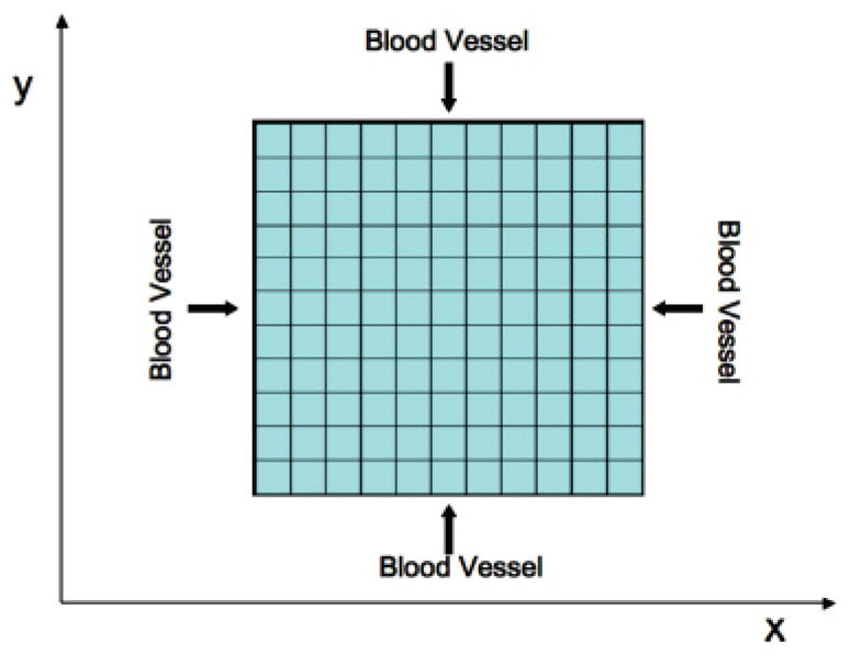
(Color online) Discretized two-dimensional host tissue. Blood vessels provide the tissue, at its borders, with proliferation and survival nutrients at a constant rate.

The simulation of this model involves two steps: In the first step, we solve a system of reaction-diffusion equations and obtain the nutrient profiles in the tissue. In the second step, the computed nutrient distributions, as well as the spatial distribution of tumor cells, are used to define the probabilities of cell-level processes, such as division, death, and migration. Each cycle of the model corresponds to the period of the tumor cell’s division cycle; the cell cycle ranges between 0.5 and 10 days depending on the cell type [45,46].

1. Reaction-diffusion equations

The reaction-diffusion equation approach has been widely used [2,4,41,47] to describe the dynamics of nutrient species as well as other cell substrates used in models of growing tumors. In the model used here [38], reaction-diffusion equations describe the dynamics of two nutrient species: one for cell mitosis and one for cell survival of both normal and tumor cells (see also [21,48]).

The nutrient species diffuse within the domain (tissue) and are also consumed by the different cell species. The dynamics of the nutrient species are determined by the following set of partial differential equations:

$$\begin{array}{l}\frac{\partial N}{\partial t}=D_N{\nabla }^{2}N-k_{1}HN-k_{2}TN,\\ \frac{\partial M}{\partial t}=D_M{\nabla }^{2}M-k_{3}HM-k_{4}TM,\end{array}$$ (1)

where N and M represent concentrations of nutrient species required for mitosis and viability, respectively, of all the cell species. The cell species under consideration are the host cells, the number of which is denoted by H, and the tumor cells, the number of which is denoted by T. D_N and D_M represent the diffusion coefficients of species N and M, respectively; k₁, k₂ are the rate coefficients of N consumption by the host and tumor cells, respectively, and k₃, k₄ are the analogous rates for the survival nutrient M.

The diffusion coefficients of the nutrient species are taken to be equal, i.e., D_N = D_M = D and similar simplifications can be applied for the nutrient consumption rates by host cells, i.e., k₁ = k₃. In order to take into account the higher consumption rate of nutrients by tumor cells, we consider this rate as a constant multiple of the consumption rate by host cells, i.e., k₂ = λ_N k₁ and k₄ = λ_M k₃, where λ_N, λ_M ≥ 1.

Nutrients are supplied through blood vessels at the boundaries of the tissue, i.e., at x = 0, x = L, y = 0, and y = L. The concentration of nutrients at the tissue boundaries is assumed to remain constant in time. Thus, the boundary conditions of (1) become

$$\begin{array}{l}N(0,y)=N(L,y)=N(x,0)=N(x,L)=N_0,\\ M(0,y)=M(L,y)=M(x,0)=M(x,L)=M_0.\end{array}$$ (2)

A set of transformations is used to nondimensionalize the set of reaction-diffusion equations (1):

$$\widehat{t}=\frac{t}{t_{\text{div}}},(\widehat{x},\widehat{y})=\left(\frac{x}{\mathrm{\Delta }},\frac{y}{\mathrm{\Delta }}\right),\widehat{N}=\frac{N}{N_0}\text{and}\widehat{M}=\frac{M}{M_0},$$ (3)

where t̂, x̂, ŷ, N̂, M̂ are dimensionless quantities; t_div is the cell division time and Δ the side length of the square element, which discretizes the computational domain. The application of transformations (3) to Eq. (1) yields the following dimensionless set of equations:

$$\begin{array}{l}\epsilon \frac{\partial N}{\partial t}={\nabla }^{2}N-a^{2}HN-{\lambda }_N{a}^{2}TN,\\ \epsilon \frac{\partial M}{\partial t}={\nabla }^{2}M-a^{2}HM-{\lambda }_M{a}^{2}TM,\end{array}$$ (4)

where, for the sake of simplicity, we drop the “ˆ” symbol; ε = (Δ²/D)/t_div is the ratio of diffusion time to division time, and is assumed to be small. The constant $a^2=\frac{k_1{\mathrm{\Delta }}^2}{D}$ is the dimensionless rate of nutrient consumption by host cells. The dimensionless boundary conditions are

$$\begin{array}{l}N(0,y)=N(L,y)=N(x,0)=N(x,L)=1,\\ M(0,y)=M(L,y)=M(x,0)=M(x,L)=1.\end{array}$$ (5)

The dynamics of nutrient species is in general much faster compared to the period of a cell cycle (ε is assumed to be small); thus, in practice we solve the steady state of Eq. (4) so that the spatial distributions of nutrient species N and M are computed from

$$\begin{array}{c}\begin{array}{ll}{\nabla }^{2}N-a^{2}HN-{\lambda }_N{a}^{2}TN\hfill & =0\hfill \\ {\nabla }^{2}M-a^{2}HM-{\lambda }_M{a}^{2}TM\hfill & =0\hfill \end{array}\}(x,y)\in \mathrm{\Omega }\backslash \partial \mathrm{\Omega },\\ N=M=1(x,y)\in \partial \mathrm{\Omega }.\end{array}$$ (6)

Equations (6) are discretized using centered finite difference approximation, and the resulting symmetric system of linear equations is solved by applying the conjugate gradient method. Next, we describe how the probabilities of the cell-level processes of cell death, cell division, and cell migration depend on the nutrient concentrations and the number of tumor cells.

2. Rules of the cellular automaton

The evolution of each tumor cell is determined by a set of rules with inherent randomness. The host cells are considered to be passive and they only contribute to the dynamics of the process through the consumption of nutrient species; thus, the cellular automaton rules model the possible processes that only tumor cells can undergo. If we also consider the effect of the immune system, cellular automaton rules can be also designed for immune cells and their interaction with tumor cells, as discussed in Ref. [38]. In the simplified version used here, only the tumor and host cells are modeled.

Following [38], at each iteration of the cellular automaton, tumor cells may undergo only one of the following processes: (a) death, (b) division, or (c) migration. That is, each cell is assigned a random number (independent of the microenvironmental conditions) that is used to determine which of these processes the cell is eligible to undergo. Once the cell’s potential fate is determined, a random subprocess is performed to determine whether the cell successfully undergoes this fate. The probability of this subprocess depends on the nutrient and cell distributions. As discussed in Ref. [38], this is a highly simplified model of real systems, in that we have assumed that the duration of the cell cycle is uniform among all cells (making it a synchronous process) and that differences in time scales of the three processes (death, division, migration) are neglected. The model could easily be extended to account for such differences (e.g., by using time subcycling), but this is beyond the scope of this paper.

B. Cell death due to lack of survival nutrients

Motivated by the fact that some tumor cells evade signals to undergo programed cell death (apoptosis) [49], we neglect apoptosis here. In particular, since immune cells are not considered here, we assume that tumor cells can undergo death only when the level of survival nutrients is low (necrosis). The probability for necrosis is given by

$$P_{\text{nec}}=exp\left[-{\left(\frac{M}{T{\theta }_{\text{nec}}}\right)}^2\right].$$ (7)

That is, the probability of necrosis increases when the level of nutrient required for cell-survival decreases, relative to the local number of tumor cells. θ_nec is a shape parameter for the probability distribution (e.g., see [21,38]). If a cell becomes necrotic, then it is designated as “necrotic material’, and remains in its current location.

C. Cell proliferation

When a tumor cell is selected for division, the probability for this to occur is

$$P_{\text{div}}=1-exp\left[-{\left(\frac{N}{T{\theta }_{\text{div}}}\right)}^2\right].$$ (8)

The probability of division is high when nutrient is plentiful compared to the number of tumor cells (N/T is large). The parameter θ_div controls the shape of the proliferation probability distribution.

If a cell is successfully selected for proliferation, its offspring is placed at one of the neighboring sites of the mother cell. The position at which the daughter cell is placed depends on the number of tumor cells already located there. If the tumor cell, chosen for division, is surrounded by at least one site occupied by a host cell, or necrotic material, then the daughter cell will be randomly placed at one of these sites and will replace the host cell or necrotic material. When all neighboring sites are occupied by tumor cells, then the offspring is placed at the site with the lowest number of tumor cells to minimize crowding.

D. Migration of tumor cells

When a tumor cell is selected for migration, we compute the corresponding probability through

$$P_{\text{mig}}=1-exp\left[-T{\left(\frac{M}{{\theta }_{\text{mig}}}\right)}^2\right].$$ (9)

The migration probability is modeled to increase with the number of tumor cells and the survival nutrient concentration M. In particular, cells tend to migrate if there is crowding and/or there are sufficient survival nutrients available (T M² increases). The parameter θ_mig controls the sensitivity of the probability distribution to T and M. For simplicity, we do not model the cells’ natural tendency to move, e.g., by random motion or chemotaxis, although these effects could be easily incorporated [50–52].

The position to which the cell migrates is chosen applying the same criteria used for the placement of an offspring in the case of cell division. When neighboring sites are occupied by host or necrotic material, then the migrating cell moves randomly to one of them; if all neighboring sites are occupied by tumor cells, it moves toward the one with the smallest number of tumor cells. This can be thought of as a simple version of Darcy’s law where the motion is in the direction of maximum decrease in cell density.

The overall computational algorithm is summarized as follows:

1. We assign values to parameters L, λ_M, λ_N, θ_nec, θ_div, θ_mig, a and we discretize the domain (tissue). We initialize the distributions of host and tumor cells in the tissue. Following [38], we start with a single tumor cell placed at the center of the tissue. The remaining lattice sites are occupied by one host cell (H = 1).

2. We solve the system of reaction-diffusion equations (6) to obtain the spatial distributions of nutrients N and M.

3. Each tumor cell is randomly assigned a potential cell fate, i.e., division, death, or migration.

4. At each site of the discretized tissue, we evaluate the probabilities of death, proliferation, or migration and determine the fate of each cell. For example, if a cell is assigned a potential death fate, and p is a random number generated uniformly in [0,1] during the subprocess, then death occurs when p < P_nec.

5. We update the distributions of host and tumor cells at each tissue site depending on the decisions made at step (iv) and we update time t.

6. We repeat steps (ii)–(v) until time t reaches a terminal value (t_fin).

E. Results obtained from direct simulation of the composite model

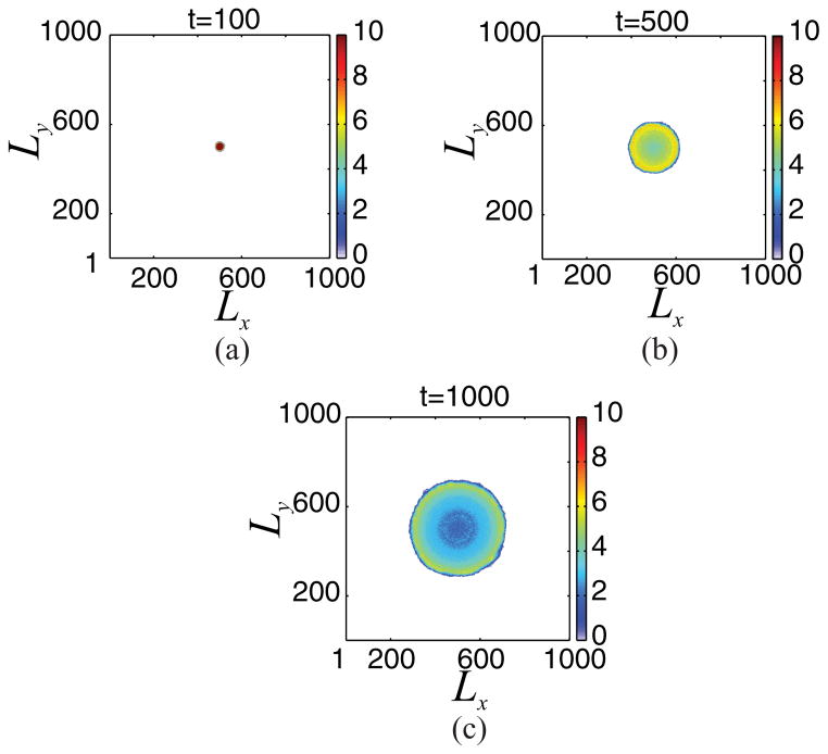
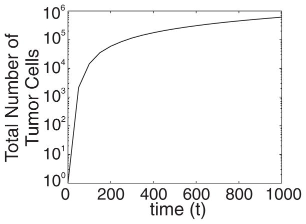
We now present results obtained from the direct simulation of the composite model presented above. In particular, Fig. 2 shows snapshots of the tumor cell distribution until time t_fin = 1000, when the following set of parameter values is used: L_x = L_y = L = 1001, θ_nec = 0.03, θ_div = 0.3, θ_mig = 1000, a = 1/L, λ_N = 25, and λ_M = 25. The simulation is repeated 20 times and we plot the mean tumor cell distribution. One can observe that the number of tumor cells is increased at the outer region of the growing tumor, which is surrounded by sites occupied by host cells. Figure 3 shows that the evolution of the total number of tumor cells exhibits an exponential increase in time.

FIG. 2.

(Color online) Results obtained from direct simulation of the cellular automaton when L_x = L_y = L = 1001, θ_nec = 0.03, θ_div = 0.3, θ_mig = 1000, a = 1/L, λ_N = 25, and λ_M = 25. Here, we show snapshots of the tumor cell distribution at dimensionless times: (a) t = 100, (b) t = 500, and (c) t = 1000. The growing tumor exhibits a (coarsely) radially symmetric shape on the coarse scale. See text for additional details.

FIG. 3.

Evolution of the total number of tumor cells of the growing tumor shown in Fig. 2.

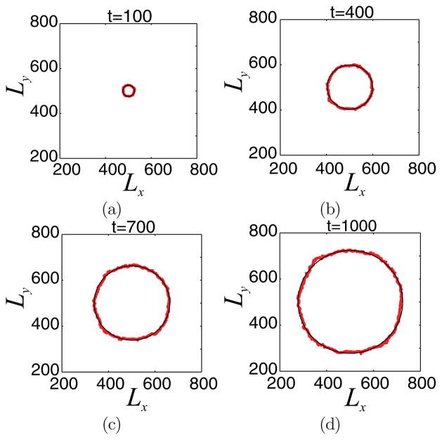
Under these conditions, the growing tumor appears to be radially symmetric (see Fig. 2), at least on a coarse scale. As discussed in Ref. [38], radially symmetry can be broken and invasive fingering can be observed if the consumption of the proliferation nutrient by tumor cells is increased relative to that of the survival nutrient. In Fig. 4, we plot the front (red line) of the developing tumor (computed from one simulation), which can be approximated by circles of growing radii (black line; the radius is equal to the mean radius of the tumor front).

FIG. 4.

(Color online) Tumor front evolution (red line) for the growing tumor shown in Fig. 2. The black line corresponds to a circular front with radius equal to the mean radius of the tumor front.

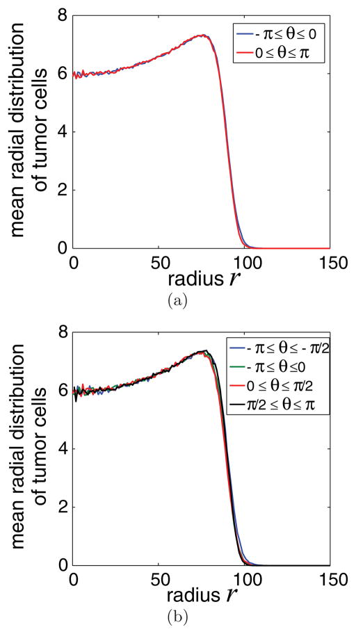
Our statement that the observed growing tumor is characterized by coarse radial symmetry is further reinforced by performing the following test. The discretized tissue is divided into circular sectors, which are constructed by computing the polar coordinates (r, θ) from the Cartesian coordinates (x,y) of each site of the domain. For example, when the tissue is divided into two circular sectors, then the first sector contains all sites with polar angles −π ≤ θ < 0; the second circular sector contains sites with polar angles 0 ≤ θ < π.

Next, we compute the mean radial distributions of tumor cells for each of the two sectors (integration of the mean radial distribution in a sector produces the number of tumor cells therein). If these distributions are “coarsely” equal, this is an indication that the developing tumor is coarsely radially symmetric. The same test can be performed for different numbers of circular sectors.

In Fig. 5, we depict the mean radial distributions of tumor cells for two different cases: when the domain is divided into (a) two circular sections and (b) four sections at time t = 400. Indeed, the mean radial distributions computed at the different sectors compare well, thus validating quantitatively our hypothesis of effective radial symmetry. Similar results are also obtained when a larger number of sectors is used, as well as for cell distributions obtained at different times. Interestingly, the observed mean radial distributions are very similar to those obtained using continuum mixture models with the cell velocity given by a version of Darcy’s law (e.g., [15]).

FIG. 5.

(Color online) Mean radial tumor cell distribution at time t = 400, when the domain is divided into (a) two sectors (−π ≤ θ ≤ 0, 0 ≤ θ ≤ π) and (b) four sectors (−π ≤ θ ≤ −π/2, − π/2 ≤ θ ≤ 0, 0 ≤ θ ≤ π/2, π/2 ≤ θ ≤ π). The mean radial distributions computed at different sectors appear “coarsely” the same, indicating the radial symmetry of the developing tumor.

Comprehensive studies of individual-based models such as this are often impeded by the large computational cost of the algorithms. In particular, large linear systems need to be solved to obtain the nutrient concentrations from the discretized (e.g., finite difference) versions of system (6) at every time step. By exploiting the symmetric character of the generated systems, we employ the conjugate gradient method. While this iterative solver minimizes the memory demands, however, the exponentially increasing number of tumor cells further increases the computational time (especially when this number exceeds 10⁶). Thus, performing comprehensive parametric studies for numerous realizations of this, and other individual-based models, is a computationally demanding task. For example, a single realization of the current, highly simplified model up to time t_fin = 1000 takes approximately 70 min on an Intel Core 2 Duo processor. In the next section, we describe the equation-free framework, where coarse-scale projective integration is used to significantly speed up the computation.

III. COARSE APPROACH OF A GROWING TUMOR WITH RADIAL SYMMETRY

A. Coarse time stepper

In the equation-free approach, a coarse-scale time stepping algorithm, the so-called coarse time stepper [32–34], is used to accurately and efficiently reduce the computational cost of simulating the system dynamics using the direct, individual-based method without explicitly prescribing the equations governing the coarse-scale dynamics. In particular, coarse-scale information can be extracted by appropriately initialized short bursts of the individual-based model. A schematic of the coarse time stepper is shown in Fig. 6. Suppose we are interested in studying the evolution of a coarse variable f. As discussed below, here f is taken to be the ensemble-averaged radial tumor cell density. Ideally, a rigorous upscaling of the discrete model should yield explicit equations governing the dynamics of the averaged cell density. However, this may be difficult to achieve and may require uncontrolled approximations to obtain explicit formulas. This is a particularly difficult problem when the microscopic models are complex. As a result, phenomenological assumptions are often employed, which can limit the predictiveness of the resulting coarse-scale system.

FIG. 6.

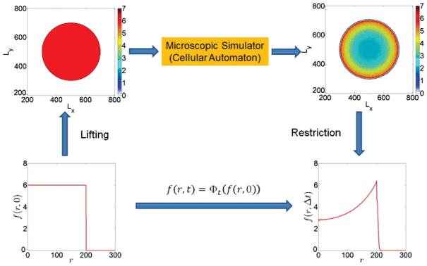
(Color online) Schematic of a coarse time stepper for the model of a growing avascular tumor with radial symmetry.

We can circumvent the need for an explicit coarse-scale description through the construction of a coarse time stepper, which wraps around the cell-level simulator and provides a discrete time map for the coarse variable f. The basic steps of this construction are described in the following (e.g., see also [33] for further details).

We denote by f (0) the initial value of the coarse variable at time t = 0; through a lifting step, we create a number of microscopic-cell distributions, consistent with f (0). The individual-based model is simulated for a short time Δt for each of the “lifted” cell distributions, resulting in updated microscopic states. The ensemble-averaged cell density f (Δt) is then constructed by averaging the updated microscopic distributions. This is called the restriction step. The derivation of an explicit expression for the evolution of f is thus bypassed; instead, a discrete time mapping is constructed utilizing short bursts of the direct individual-based model.

The lifting and restriction steps are problem-dependent procedures. In this particular problem of a growing tumor, its radial symmetry suggests that an “appropriate” coarse observable can be the ensemble-averaged (e.g., mean) radial density (distribution) of tumor cells f (r,t), where r is the radial distance of a tissue site from the tumor center. Thus, our purpose is (a) to develop a lifting operator which creates cell distributions consistent with a value f (r,t) and then (b) develop a restriction operator which computes the ensemble-average variable f (r,t) of tumor cell density in the tissue. Below, we describe the lifting and restriction algorithms in some detail.

1. Lifting

We discretize the computational domain (tissue) using L × L sites (nodes) at which the reaction-diffusion equations (6) are solved for the nutrient species concentrations (N and M). These nodes are the centers of square elements within which tumor cells, host cells, or necrotic material reside. In the results shown below, L_x = L_y = L = 1001. Each node is characterized by a pair of Cartesian coordinates (i,j) (i,j = 1, …, L). The coordinates at the center of the tissue are (i₀,j₀) = (501,501). The Cartesian coordinates are then transformed to polar coordinates (r_i,j, θ_i,j). The mean radial distribution of the tumor cells is computed in the domain r ∈ [0, R_max], with R_max = 500. The interval [0, R_max] is discretized using 501 points, e.g., the distance between two successive points in the discretized interval of the radial domain r is δ R = 1.

The mean radial distribution of the tumor cells f (r) is available in discrete form, e.g., its value f_k is available at radial distances r_k. Then, we assign the value f_k to the sites satisfying the constraint r_k − δR/2 ≤ r_i,j ≤ r_k + δR/2. If N_s is the number of the sites satisfying this constraint, then we construct a N_s -dimensional vector of random numbers, created from a Gaussian distribution with mean value f_k and standard deviation 0.1 f_k. Finally, the rounded integer values of this vector are assigned to each of the N_s sites.

These microscale cell states are consistent with the macroscopic variable f (r) and are used as initial conditions for the individual-based algorithm. The composite model is simulated for a relatively short time period denoted by Δt. Upon completion, the new distribution of tumor cells is obtained, and the corresponding mean radial tumor cell density is computed using the restriction algorithm, which is described in the following.

2. Restriction

The restriction algorithm involves the computation of the mean radial tumor cell density f (r), i.e., the computation of values f_k at radii r_k. Initially, we locate the locus of domain sites, with coordinates satisfying the constraint r_k − δR/2 ≤ r_i,j ≤ r_k + δR/2. The value of f_k is then computed as the mean value of the tumor cells at sites which satisfy the constraint above, i.e., f_k = mean(T_i,j), where T_i,j is the number of tumor cells at the site with coordinates (i,j). Finally, we average over all the computed microscopic states.

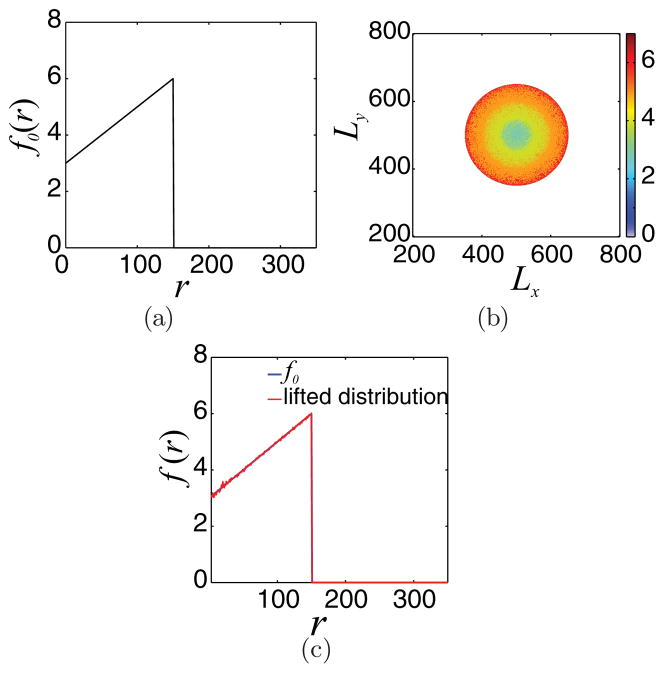
The restriction step is effectively the inverse of the lifting procedure. To verify this, we produce microscopic distributions through the lifting process given a mean radial distribution f₀; then, we test whether the restriction of the produced microscopic distributions produces a mean radial distribution f_lift, which is coarsely equal with f₀, e.g., f_lift ≈ f₀. The results are shown in Fig. 7(c), where it is clear that the proposed lifting and restriction procedures produce “coarsely” the same macroscopic distributions f (r); f₀ for this example was chosen to be

FIG. 7.

(Color online) (a) Initial mean radial tumor cell density f₀ given by the expression in Eq.(10). (b) One microscopic cell distribution consistent with f₀. (c) f_lift (red broken line) is the restriction of the distribution in figure (b), lifted from f₀. Comparing f_lift with the initial distribution f₀ (blue solid line) demonstrates that the restriction operation is the (coarse) approximate inverse of the lifting step.

$$f_0(r)=\frac{1}{50}r+3,r\le 150.$$ (10)

The precise form of f₀ is not important; f_lift ≈ f₀ in all cases tested.

IV. COARSE PROJECTIVE INTEGRATION IN A COMOVING FRAME

The coarse-scale time stepper effectively approximates the time mapping

$$f(t)={\mathrm{\Phi }}_t(f(0)).$$ (11)

This enables the execution of time-stepper-based algorithms, without requiring the explicit knowledge of the operator Φ_t.

Here, we apply the coarse projective integration method, which enables the acceleration of temporal computations. This approach exploits the fact that the coarse variable evolves more slowly and smoothly than the microscopic variables. We therefore utilize the coarse time stepper to approximate the time derivatives of the mean radial tumor cell density f (the macroscopic variable), which are used in time projection schemes [35,36]. A few calls of the coarse time stepper produce a series of coarse variable values at discrete time steps, which are also incorporated in the time projection scheme. We now outline the details.

It turns out that it is more convenient to work with differences (e.g., scaled discrete derivatives) h of the mean radial tumor cell density. That is,

$$h_j=\{\begin{array}{ll}{f}_j-0\hfill & \text{for}j=501,\hfill \\ f_{j+1}-f_j\hfill & \text{for}j=1,\dots ,500.\hfill \end{array}$$ (12)

Since h is zero at r = 0 (by symmetry) and at r = R_max (this is beyond the tumor), it can be represented as a truncated Fourier series [53]

$$h(r)\approx \frac{a_0}{2}+\sum _{k=1}^K\left(a_{k}cos\left[\frac{k2\pi r}{R_{max}}\right]+b_{k}sin\left[\frac{k2\pi r}{R_{max}}\right]\right),$$ (13)

where a_m, m = 0, …, K, and b_j, j = 1, …, K, are the Fourier coefficients. Assuming we have an estimate for the time derivative of the Fourier coefficients, we can use the forward Euler method to approximate the Fourier coefficients at a later time (t_project). To approximate the time derivative, we can use a divided difference of the Fourier coefficients at two times t₁ and t₂. Thus, the projection of the Fourier series coefficients at time t_project is estimated from

$$\begin{array}{l}{a}_{m,t_{\text{project}}}\approx a_{m,t_2}+{\frac{\partial a_m}{\partial t}|}_{t_2}(t_{\text{project}}-t_2)\\ \approx a_{m,t_2}+\frac{a_{m,t_2}-a_{m,t_1}}{t_2-t_1}(t_{\text{project}}-t_2),\\ b_{j,t_{\text{project}}}\approx b_{j,t_2}+{\frac{\partial b_j}{\partial t}|}_{t_2}(t_{\text{project}}-t_2)\\ \approx b_{j,t_2}+\frac{b_{j,t_2}-b_{j,t_1}}{t_2-t_1}(t_{\text{project}}-t_2).\end{array}$$ (14)

Using the values of the projected Fourier coefficients, the distribution h(r,t_project) is computed from Eq.(13). Finally, the projection of the mean radial tumor cell density f (r,t_project) is obtained from

$$f_j=\{\begin{array}{ll}0\hfill & \text{for}j=501,\hfill \\ f_{j+1}-h_j\hfill & \text{for}j=1,\dots ,500.\hfill \end{array}$$ (15)

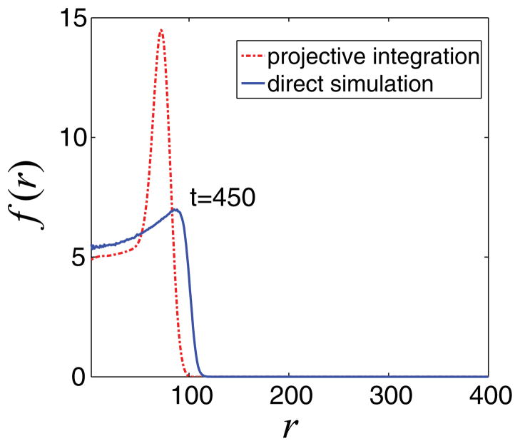
In Fig. 8, we present the results of this algorithm when t₁ = 300, t₂ = 350, and the projection time is t_project = 450. Comparing the projected mean density with that obtained from a direct simulation of the individual-based model shows that the algorithm as described above does not produce results of acceptable accuracy.

FIG. 8.

(Color online) Comparison of mean radial density of tumor cells at time t = 450, obtained by direct simulations (blue line) and coarse projective integration (red line). The (clearly erroneous) result of simple (non-comoving frame) coarse projective integration is obtained using t₁ = 300, t₂ = 350, and t_project = 450 with K = 50 Fourier coefficients.

This failure is not due to insufficient Fourier discretization. In particular, we perform the following test: We consider the mean radial tumor cell density at time t = 500 and compute its first K = 50 Fourier coefficients. Then, we compare the original distribution f (r,500) with the truncated distribution resulting from the application of Eqs. (13) and (15), f_Fourier(r,500). As can be seen in Fig. 9, the differences in the two distributions are indistinguishable. The same observation holds for distributions obtained at other times.

FIG. 9.

(Color online) Mean radial density of tumor cells (blue line) at t = 500 and the corresponding distribution produced by a 50 Fourier mode truncation (red broken line). The two distributions visually coincide.

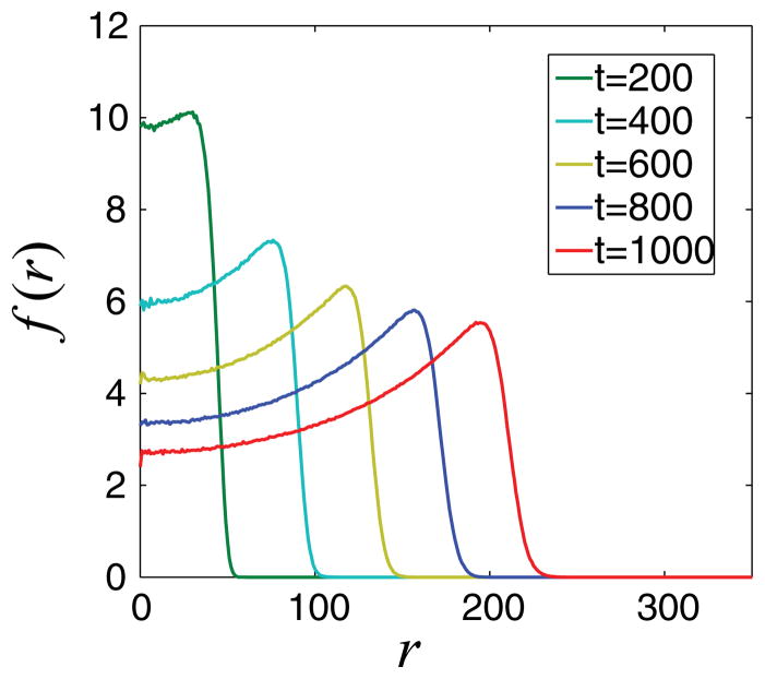
One can increase the accuracy by reducing the projection time; however, this also significantly reduces the computational savings. The main reason for the failure of this simple projective integration method is that it does not take into account the traveling character of the mean tumor cell density (see Fig. 10). We can modify accordingly the projective integration method and perform the computations in a comoving frame. An analogously modified projective integration scheme was implemented previously in Ref. [37], where it was shown that this approach enables the application of larger projection steps, thus further accelerating the temporal computations while preserving the accuracy of results.

FIG. 10.

(Color online) Evolution of the mean radial distribution of tumor cells f (r). We observe that the evolution is characteristic of a moving front.

When performing the computations in a comoving frame, traveling is factored out; the time derivative of the coarse variable (required for the application of projection schemes) is also computed in this comoving frame and represents the changes of only the shape of the traveling solution. Thus, the projection is smoother and more accurate compared to the one which does not take into account the traveling character of the solution.

Here, the modified projective integration application requires the computation of the Fourier series coefficients and their time derivatives in a comoving frame. Because we do not know the speed of the traveling front explicitly, we obtain a numerical approximation of it by maximizing the overlap of the evolved solution with an (arbitrarily chosen) “template” function, e.g., see also [54].

In our computations, a convenient choice is the trigonometric template function T̃ (r) = 1 − cos[2π r/R_max]. We seek the shift c, which maximizes the overlap between the shifted ĥ(r) = h(r + c) and the template T̃ (e.g., maximize ${\int }_0^{R_{max}}{[\widehat{h}(r)-\stackrel{\sim }{T}(r)]}^{2}dr$). The resulting algebraic constraint for the shift computation is

$$\frac{2\pi c(t)}{R_{max}}=arctan\left[\frac{b_{1,t}}{a_{1,t}}\right].$$ (16)

Using the same procedure as in the projective integration scheme described above, we obtain the Fourier series coefficients of the difference distributions h(r,t₁) and h(r,t₂) at reporting times t₁ and t₂, respectively. We emphasize that this involves the restriction of the computed tumor cell distributions from the individual-based model at these reporting times, resulting in the mean radial distributions f (r,t₁) and f (r,t₂). Then, the two difference distributions are obtained from Eq.(12), and finally the Fourier coefficients a_m,ti and b_j,ti of the h distributions are computed (m = 0, …, K, j = 1, …, K, and i = 1,2). We apply Eq. (16) and calculate the shifts c₁ = c(t₁), c₂ = c(t₂), from which we also compute the Fourier coefficients of the shifted distributions ĥ (i.e., the Fourier coefficients in the comoving frame), according to

$$\begin{array}{l}{\widehat{a}}_j=a_{j}cos\left[j\frac{2\pi c(t)}{R_{max}}\right]+b_{j}sin\left[j\frac{2\pi c(t)}{R_{max}}\right],\\ {\widehat{b}}_j=-a_{j}sin\left[j\frac{2\pi c(t)}{R_{max}}\right]+b_{j}cos\left[j\frac{2\pi c(t)}{R_{max}}\right].\end{array}$$ (17)

Then, the projection of the shifted coefficients â_j, b̂_j is computed from

$$\begin{array}{l}{\widehat{a}}_j(t_{\text{project}})={\widehat{a}}_j(t_2)+(t_{\text{project}}-t_2)\frac{{\widehat{a}}_j(t_2)-{\widehat{a}}_j(t_1)}{t_2-t_1},\\ {\widehat{b}}_j(t_{\text{project}})={\widehat{b}}_j(t_2)+(t_{\text{project}}-t_2)\frac{{\widehat{b}}_j(t_2)-{\widehat{b}}_j(t_1)}{t_2-t_1}\text{for}j=0,\dots ,K.\end{array}$$ (18)

The projection of the shift is also computed:

$$c_{\text{project}}=c_2+(t_{\text{project}}-t_2)\frac{c_2-c_1}{t_2-t_1}.$$ (19)

This enables the computation of the Fourier components of h(r,t_project), which evolves in the original frame (i.e., not comoving) as

$$\begin{array}{l}{a}_j(t_{\text{project}})={\widehat{a}}_j(t_{\text{project}})\text{cos}\left[j\frac{2\pi c_{\text{project}}}{R_{max}}\right]-{\widehat{b}}_j(t_{\text{project}})\text{sin}\left[j\frac{2\pi c_{\text{project}}}{R_{max}}\right],\\ b_j(t_{\text{project}})={\widehat{a}}_j(t_{\text{project}})\text{sin}\left[j\frac{2\pi c_{\text{project}}}{R_{max}}\right]+{\widehat{b}}_j(t_{\text{project}})\text{cos}\left[j\frac{2\pi c_{\text{project}}}{R_{max}}\right].\end{array}$$ (20)

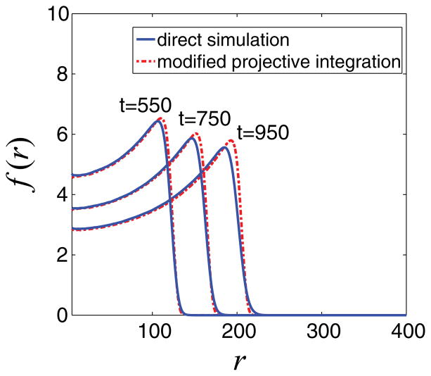
Finally, from Eq. (15) we compute the projection of the mean radial distribution f (r,t_project). In Fig. 11, we show the results of the application of the appropriately modified, comoving frame projective integration, when t₂ − t₁ = 50 and t_project − t₂ = 100. The t₂ − t₁ and t_project − t₂ values have been chosen so as to be equal to that used in the nonadjusted projective integration application (Fig. 8) when the traveling character of the solution has not been taken into account. This allows us to compare the efficacy of the projection schemes on the same basis and demonstrate the enhanced performance of the modified projective integration in the comoving frame. Indeed, comparing the mean radial tumor densities as obtained from direct simulation and from the modified projective integration method at times t = 550, 750, and 950 shows good visual agreement (Fig. 11).

FIG. 11.

(Color online) Comparison of mean radial density of tumor cells at times t = 550, 750, and 950. The blue line corresponds to the results obtained from direct simulation, and with red broken lines we depict the results of the coarse projective integration application in a comoving frame with t₂ − t₁ = 50 and t_project − t₂ = 100 using K = 50 Fourier coefficients. Good visual agreement is observed.

The choice of t₂ − t₁ = 50 and t_project − t₂ = 100 reduces substantially the required computational time, while the accuracy of computations is preserved at a high level. As reported above, the computational time for a single direct simulation is 70 min in a Core 2 Duo Intel processor. The “comoving” projective integration scheme application doubles the speed of computation (requires approximately 35 min of computational time). The shape and the position of the evolving front of the mean radial distribution of tumor cells both agree with the results obtained from direct simulation, suggesting that the proposed computational scheme can indeed serve for the more efficient study of cell-level models.

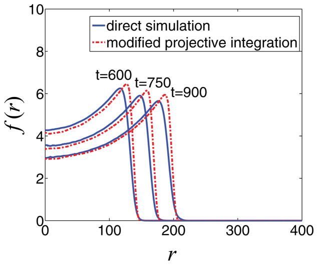
We can further increase the computational savings by increasing the ratio (t_project − t₂)/(t₂ − t₁). In Fig. 12, we compare the mean radial tumor densities obtained from direct simulation of the composite model and the modified projective integration method at times t = 600, 750, and 900, when savings are increased significantly (four times faster with projective integration), while the accuracy of computations is still preserved at a high level, although the simulations are not as accurate as those shown in Fig. 11, where (t_project − t₂)/(t₂ − t₁) = 2. As is typical, decreased computational cost is accompanied by a small loss in accuracy.

FIG. 12.

(Color online) Comparison of mean radial density of tumor cells at times t = 600, 750, and 900. The blue lines correspond to the results obtained from direct simulation, and with red broken lines we depict the results of the application of coarse projective integration in a comoving frame with t₂ − t₁ = 25 and t_project − t₂ = 100 using K = 50 Fourier coefficients. t_project − t₂ = 100 and t₂ − t₁ = 25. Here, the computational

V. CONCLUSIONS

In this paper, we have presented a proof-of-principle computational approach that can be used to help bridge the gap between tissue scale models of tumor growth, usually described by continuum theory, and cell and subcell scale models, that typically utilize stochastic, individual-based algorithms. Continuum models can be studied using traditional techniques for partial differential equations, however, they typically rely on phenomenological assumptions rather than being the result of rigorous upscaling of microscopic systems. This can make predictions of such continuum models unreliable. On the other hand, individual-based models capture the detailed dynamics of cells and their interactions, but their computational cost makes it difficult to simulate very large systems and perform extensive parameter studies, which are needed to predict large-scale tumor dynamics and to design and predict the outcome of anticancer therapies.

Rather than performing an analytical upscaling of an individual-based model, we have used the equation-free framework, and coarse projective integration in particular, to accelerate a cellular automaton model that describes the detailed dynamics of individual cells. This is an important step toward making long-time multiparameter studies of individual-based models feasible. Here, we examined the case of a growing tumor, the coarse scale integration of which is radially symmetric. By performing projective integration in a frame that is comoving, we can achieve high accuracy computations (compared to the direct simulation results) and significant computational savings.

Our analysis can be extended for nonradially symmetric tumors. In asymmetric cases, the mean tumor cell density is still a good candidate for the coarse-scale variable except that now variability in r and θ (polar angle), e.g., f = f (r, θ), needs to be considered. The design of a comoving frame is more difficult in this asymmetric case, although there are several possibilities for doing this (see Refs. [55,56]); this is currently under study. Additional computational savings can be achieved by applying the so-called gap tooth scheme [33,57], which limits fine scale simulations to a collection of small adaptively selected boxes throughout the domain, rather than simulating the individual-based model over the entire domain. These fine simulations can be used to generate macroscale fluxes that enable communication between boxes to simulate processes, e.g., convection and diffusion, operating on the coarse scales.

References

- 1.Weinberg RA. Sci Am. 1996;275:62. doi: 10.1038/scientificamerican0996-62. [DOI] [PubMed] [Google Scholar]
- 2.Lowengrub JS, Frieboes HB, Jin F, Chuang YL, Li X, Macklin P, Wise SM, Cristini V. Nonlinearity. 2010;23:R1. doi: 10.1088/0951-7715/23/1/r01. [DOI] [PMC free article] [PubMed] [Google Scholar]
- 3.Byrne HM. Nat Rev Cancer. 2010;10:221. doi: 10.1038/nrc2808. [DOI] [PubMed] [Google Scholar]
- 4.Anderson ARA, Quaranta V. Nat Rev Cancer. 2008;8:227. doi: 10.1038/nrc2329. [DOI] [PubMed] [Google Scholar]
- 5.Adam JA. Math Biosci. 1986;81:229. [Google Scholar]
- 6.Tracqui P, Cruywagen GC, Woodward DE, Bartoo GT, Murray JD, Alvord ECJ. Cell Proliferation. 1995;28:17. doi: 10.1111/j.1365-2184.1995.tb00036.x. [DOI] [PubMed] [Google Scholar]
- 7.Woodward DE, Cook J, Tracqui P, Cruywagen GC, Murrayand JD, Alvord ECJ. Cell Proliferation. 1996;29:269. doi: 10.1111/j.1365-2184.1996.tb01580.x. [DOI] [PubMed] [Google Scholar]
- 8.Ward JP, King JR. Math Med Biol. 2003;14:39. doi: 10.1093/imammb/20.3.227. [DOI] [PubMed] [Google Scholar]
- 9.Byrne HM, Chaplain MAJ. Math Biosci. 1995;130:151. doi: 10.1016/0025-5564(94)00117-3. [DOI] [PubMed] [Google Scholar]
- 10.Byrne HM, Chaplain MAJ. Eur J Appl Math. 1997;8:639. [Google Scholar]
- 11.Owen MR, Sherratt JA. J Theor Biol. 1997;189:63. doi: 10.1006/jtbi.1997.0494. [DOI] [PubMed] [Google Scholar]
- 12.Pettet GJ, Please CP, Tindall MJ, McElwain DLS. Bull Math Biol. 2001;63:231. doi: 10.1006/bulm.2000.0217. [DOI] [PubMed] [Google Scholar]
- 13.Cristini V, Lowengrub J, Nie Q. J Math Biol. 2003;46:191. doi: 10.1007/s00285-002-0174-6. [DOI] [PubMed] [Google Scholar]
- 14.Wise SM, Lowengrub JS, Frieboes HB, Cristini V. J Theor Biol. 2008;253:524. doi: 10.1016/j.jtbi.2008.03.027. [DOI] [PMC free article] [PubMed] [Google Scholar]
- 15.Cristini V, Li X, Lowengrub JS, Wise SM. J Math Biol. 2009;58:723. doi: 10.1007/s00285-008-0215-x. [DOI] [PMC free article] [PubMed] [Google Scholar]
- 16.Frieboes HB, Jina F, Chuang YL, Wise SM, Lowengrub JS, Cristini V. J Theor Biol. 2010;264:1254. doi: 10.1016/j.jtbi.2010.02.036. [DOI] [PMC free article] [PubMed] [Google Scholar]
- 17.Pham K, Frieboes HB, Cristini V, Lowengrub J, Soc JR. Interface. 2011;8:16. doi: 10.1098/rsif.2010.0194. [DOI] [PMC free article] [PubMed] [Google Scholar]
- 18.Alarcon T, Byrne HM, Maini PK. J Theor Biol. 2003;225:257. doi: 10.1016/s0022-5193(03)00244-3. [DOI] [PubMed] [Google Scholar]
- 19.Dormann S, Deutsch A. In Silico Biol. 2002;2:0035. [PubMed] [Google Scholar]
- 20.Ermentrout GB, Edelstein-Keshet L. J Theor Biol. 1993;160:97. doi: 10.1006/jtbi.1993.1007. [DOI] [PubMed] [Google Scholar]
- 21.Ferreira SC, Jr, Martins ML, Vilela MJ. Phys Rev E. 2002;65:021907. doi: 10.1103/PhysRevE.65.021907. [DOI] [PubMed] [Google Scholar]
- 22.Kansal AR, Torquato S, Harsh GR, IV, Chiocca EA, Deisboeck TS. J Theor Biol. 2000;203:367. doi: 10.1006/jtbi.2000.2000. [DOI] [PubMed] [Google Scholar]
- 23.Patel AA, Gawlinski ET, Lemiueux SK, Gatenby RA. J Theor Biol. 2001;213:315. doi: 10.1006/jtbi.2001.2385. [DOI] [PubMed] [Google Scholar]
- 24.Drasdo D, Höhme S. Phys Biol. 2005;2:133. doi: 10.1088/1478-3975/2/3/001. [DOI] [PubMed] [Google Scholar]
- 25.Cheng G, Youssef BB, Markenscoff P, Zygourakis K. Biophys J. 2006;90:713. doi: 10.1529/biophysj.105.063701. [DOI] [PMC free article] [PubMed] [Google Scholar]
- 26.Lee DS, Rieger H, Bartha K. Phys Rev Lett. 2006;96:058104. doi: 10.1103/PhysRevLett.96.058104. [DOI] [PubMed] [Google Scholar]
- 27.Anderson AR, Rejniak KA, Gerlee P, Quaranta V. J Math Biol. 2009;58:579. doi: 10.1007/s00285-008-0210-2. [DOI] [PMC free article] [PubMed] [Google Scholar]
- 28.Sottoriva A, Vermeulen L, Tavaré S. PLoS Comput Biol. 2011;7:e1001132. doi: 10.1371/journal.pcbi.1001132. [DOI] [PMC free article] [PubMed] [Google Scholar]
- 29.Kim Y, Stolarska MA, Othmer HG. Math Models Methods Appl Sci. 2007;17:1773. [Google Scholar]
- 30.Wang Z, Zhang L, Sagotsky J, Deisboeck TS. Theor Biol Med Model. 2007;4:50. doi: 10.1186/1742-4682-4-50. [DOI] [PMC free article] [PubMed] [Google Scholar]
- 31.Macklin P, Edgerton ME, Thompson AM, Cristini V. J Theor Biol. 2012;301:122. doi: 10.1016/j.jtbi.2012.02.002. [DOI] [PMC free article] [PubMed] [Google Scholar]
- 32.Theodoropoulos K, Qian YH, Kevrekidis IG. Proc Natl Acad Sci U S A. 2000;97:9840. doi: 10.1073/pnas.97.18.9840. [DOI] [PMC free article] [PubMed] [Google Scholar]
- 33.Kevrekidis IG, Gear CW, Hyman JM, Kevrekidis PG, Runborg O, Theodoropoulos C. Commun Math Sci. 2003;1:707. [Google Scholar]
- 34.Kevrekidis IG, Gear CW, Hummer G. AIChE J. 2004;50:1346. [Google Scholar]
- 35.Gear CW. NEC Research Institute Technical Report No 2001-130. 2001. (unpublished) [Google Scholar]
- 36.Rico-Martínez R, Gear CW, Kevrekidis IG. J Comput Phys. 2004;196:474. [Google Scholar]
- 37.Kavousanakis ME, Erban R, Boudouvis AG, Gear CW, Kevrekidis IG. J Comput Phys. 2007;225:382. [Google Scholar]
- 38.Mallet DG, De Pillis LG. J Theor Biol. 2006;239:334. doi: 10.1016/j.jtbi.2005.08.002. [DOI] [PubMed] [Google Scholar]
- 39.Folkman J, Hochberg M. J Exp Med. 1973;138:745. doi: 10.1084/jem.138.4.745. [DOI] [PMC free article] [PubMed] [Google Scholar]
- 40.Sutherland RM. Science. 1988;240:177. doi: 10.1126/science.2451290. [DOI] [PubMed] [Google Scholar]
- 41.Greenspan HP. Stud Appl Math. 1972;51:317. [Google Scholar]
- 42.Carmeliet P, Jain RK. Nature (London) 2000;407:249. doi: 10.1038/35025220. [DOI] [PubMed] [Google Scholar]
- 43.Gerlee P, Anderson ARA. Phys Rev E. 2007;75:051911. doi: 10.1103/PhysRevE.75.051911. [DOI] [PubMed] [Google Scholar]
- 44.Lin AH. Discret Contin Dyn S, Ser B. 2004;4:241. [Google Scholar]
- 45.Byrne HM. Using Mathematics to Study Solid Tumour Growth; Proceedings of the Ninth General Meeting of European Women in Mathematics; New York: Hindawi Publishing Corporation; 2001. pp. 81–107. [Google Scholar]
- 46.Riedel H. In: The Cancer Handbook. Alison MR, editor. Wiley; New York: 2004. [Google Scholar]
- 47.Burden T, Ernstberger J, Fister KR. Discret Contin Dyn S, Ser B. 2004;4:135. [Google Scholar]
- 48.Ferreira SC, Martins ML, Vilela MJ. Phys Rev E. 2003;67:051914. doi: 10.1103/PhysRevE.67.051914. [DOI] [PubMed] [Google Scholar]
- 49.Hanahan D, Weinberg R. Cell. 2000;100:57. doi: 10.1016/s0092-8674(00)81683-9. [DOI] [PubMed] [Google Scholar]
- 50.Stein AM, Demuth T, Mobley D, Berens M, Sander LM. Biophys J. 2007;92:356. doi: 10.1529/biophysj.106.093468. [DOI] [PMC free article] [PubMed] [Google Scholar]
- 51.Khain E, Schneider-Mizell CM, Nowicki MO, Chiocca EA, Lawler SE, Sander LM. Europhys Lett. 2009;88:28006. [Google Scholar]
- 52.Khain E, Katakowski M, Hopkins S, Szalad A, Zheng X, Jiang F, Chopp M. Phys Rev E. 2011;83:031920. doi: 10.1103/PhysRevE.83.031920. [DOI] [PubMed] [Google Scholar]
- 53.Moeller J, Runborg O, Kevrekidis P, Lust K, Kevrekidis I. J Bifurcation Chaos. 2005;15:975. [Google Scholar]
- 54.Rowley CW, Kevrekidis IG, Marsden JE, Lust K. Nonlinearity. 2003;16:1257. [Google Scholar]
- 55.Li S, Lowengrub JS, Leo PH. J Comput Phys. 2007;225:554. [Google Scholar]
- 56.Beyn WJ, Selle S, Thuemmler V. SIAM J Appl Dyn Syst. 2008;7:577. [Google Scholar]
- 57.Samaey G, Roose D, Kevrekidis IG. Multiscale Model Simul. 2005;4:278. [Google Scholar]