Investigating a continuous shear strain function for depth-dependent properties of native and Tissue Engineering cartilage using pixel-size data

Abstract

A previously developed novel imaging technique for determining the depth dependent properties of cartilage in simple shear is implemented. Shear displacement is determined from images of deformed lines photobleached on a sample, and shear strain is obtained from the derivative of the displacement. We investigated the feasibility of an alternative systematic approach to numerical differentiation for computing the shear strain that is based on fitting a continuous function to the shear displacement. Three models for a continuous shear displacement function are evaluated: polynomials, cubic splines, and nonparametric locally weighted scatter plot curves. Four independent approaches are then applied to identify the best-fit model and the accuracy of the first derivative. One approach is based on the Akaiki Information Criteria, and the Bayesian Information Criteria. The second is based on a method developed to smooth and differentiate digitized data from human motion. The third method is based on photobleaching a predefined circular area with a specific radius. Finally, we integrate the shear strain and compare it with the total shear deflection of the sample measured experimentally. Results show that 6^th and 7^th order polynomials are the best models for the shear displacement and its first derivative. In addition, failure of tissue-engineered cartilage, consistent with previous results, demonstrates the qualitative value of this imaging approach.

1. Introduction

Native articular cartilage (AC) has a unique stratified structure and composition, which gives rise to depth-dependent mechanical properties (Buckley et al., 2010; Buckley et al., 2008; Buckwalter and Mankin, 1997; Chen et al., 2001; Lopez et al., 2008). Structure and composition also vary during maturation and are thought to influence the function of cartilage in vivo (Canal et al., 2008; Hunziker et al., 2007). In contrast, Tissue Engineered (TE) cartilage that is being developed as a potential treatment for damaged articular cartilage lacks the compositions, structure and mechanical properties of native tissue. Such differences could limit the clinical success of an implanted construct where it must function in the highly loaded environment of a diarthrodial joint. Properly functioning TE cartilage may require the depth-dependent zonal architecture and composition of native tissue.

Previous studies in our labs showed failure of TE cartilage under combined cyclic shear and static compressive loads, while native cartilage remained intact when tested under the same conditions (Jayaraman, 2010; Whitney et al., 2010a; Wong and Sah, 2010). Subsequent investigations identified a cell rich (matrix deficient) region in the middle layer of TE cartilage. From these and other studies, it’s clear that the depth-dependent properties of TE cartilage do not replicate those of native tissues (Whitney et al., 2010a; Whitney et al., 2012a). These observations provided the motivation for investigating depth-dependent properties of native and TE cartilage, which may play an important role in understanding how cartilage function is related to zonal arrangement.

Depth-dependent properties of AC are often evaluated using methods based on optical imaging. Methods that depend on tracking the displacement of low-density markers such as chondrocytes may limit spatial resolution of material properties (Buckley et al., 2010; Buckley et al., 2008; Wong et al., 2008a; Wong et al., 2008b). An alternative, with potentially higher resolution, is to track lines photobleached on the tissue (Bruehlmann et al., 2004; Buckley et al., 2010). All of these techniques require cutting the tissue to expose a surface through its thickness, which is then imaged (Bruehlmann et al., 2004; Buckley et al., 2010; Buckley et al., 2008; Canal et al., 2008; Hosoda et al., 2008; Schinagl et al., 1997). In all of these approaches, digitizing the displacement of features introduces noise, and computing the derivative of the shear displacement field (i.e. shear strain) introduces additional noise into the final estimate of material properties. Typically, some level of smoothing is needed to minimize the effects of noise and produce usable results. For example, Buckley et al., chose to smooth data by using average intensity across rectangular 20 µm deep regions, and then calculated the shear strain using numerical differentiation. Since numerical differentiation increases noise, they introduced weighting schemes that reduced noise (Buckley et al., 2010). Choosing a region that was greater or less than 20 µm, or choosing different weighting factors would have produced smoother or noisier results. Since noise is inherent in experimental measurements and numerical differentiation, determining a level of smoothing that produces accurate results is an ongoing issue (Lesh et al., 1979; Pezzack et al., 1977; Winter et al., 1974).

Based on our previous experience with failure of tissue engineered cartilage and a general interest in mechanical evaluation of native and tissue engineered cartilage, we implemented an experimental approach for determining depth dependent shear properties of cartilage similar to that described in (Buckley et al., 2010). Initial measurements showed that the full thickness deformation field for native articular cartilage in shear resembled a smooth, sigmoid-shaped curve. This raised the possibility of modeling the displacement field and shear strain using analytical functions rather than the common approach which is to smooth the data use numerical differentiation. Therefore, the purpose of this investigation was to validate a systematic method for processing displacement data and taking its first derivative. As a result, in this study, we investigate the feasibility of using a continuous, depth-dependent displacement function calculated from high-resolution pixel-dependent displacement data, and calculate shear strain by taking its first derivative analytically, thereby eliminating the noise due to numerical differentiation. This method was validated by comparison with known results.

2. Materials and Methods

2.1. Bovine AC

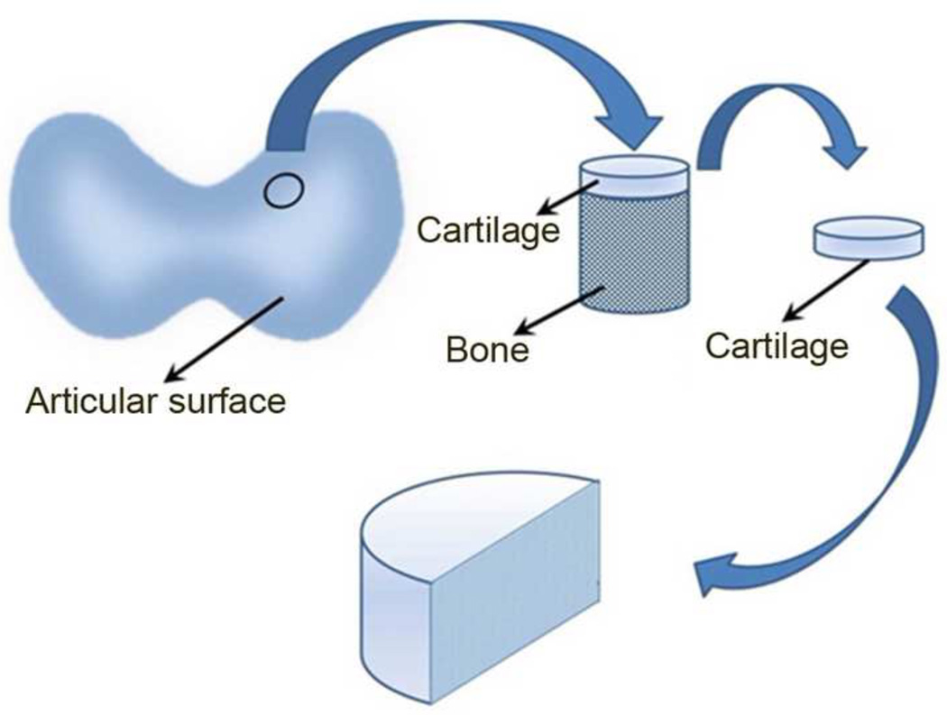
Native bovine AC was used during the development of the image processing technique. Samples were harvested from femoral condyle of a 2-year-old cow (n = 7, Halal Meat, Cleveland, OH). Osteochondral samples were removed from the whole bone using a 6 mm diameter-coring tool. Cartilage disks are then removed from the core using a scalpel, and bisected into semi-cylinders and frozen once prior to use (Fig. 1).

Fig. 1. Schematic of sample preparation for native AC biaxial mechanical testing.

Cartilage disk is removed from the 6 mm diameter bone plug, and bisected into semi-cylinders.

2.2. Tissue Engineered Cartilage

To investigate a possible failure mechanism identified in previous investigations (Whitney et al., 2010a). Scaffold-free engineered cartilage constructs were generated. Briefly, rabbit articular chondrocytes were isolated and culture expanded as described (Whitney et al., 2012b). Four cartilage sheets were formed after second passage, by seeding 3.125×10⁶ cells, onto porous (10 µm pore diameter) polyester membranes (PET1009030, Sterlitech, Kent, WA) held in place and submerged in medium by custom 4 cm × 4 cm chambers (Weidenbecher et al., 2008; Whitney et al., 2012b). Constructs were cultured for four weeks in the chambers then transferred to 100 mm petri dishes where they were allowed to float freely for an additional four weeks (Whitney et al., 2010a; Whitney et al., 2010b; Whitney et al., 2012a). The resulting TE cartilage sheet was cut into 4 mm × 6 mm rectangular samples to fit into the heads of holding arms of the apparatus, and frozen.

2.3. Staining Procedure

Before mechanical testing, samples were placed in Phosphate Buffered Saline (PBS) until thawed, and then incubated in PBS containing a 7 µg/mL solution of the fluorescent dye 5-dichlorotriazinylaminofluorescein (5-DTAF) (Invitrogen, Eugene, OR) for 2h. 5-DTAF modifies amines in proteins and fully stains the extracellular matrix. Its maximum excitation and emission wavelength are 492 nm and 520 nm (Benchaib et al., 1996). Previous studies showed that 5-DTAF does not affect the mechanical properties of cartilage (Bruehlmann et al., 2004; Buckley et al., 2010).

2.4. Mechanical Testing

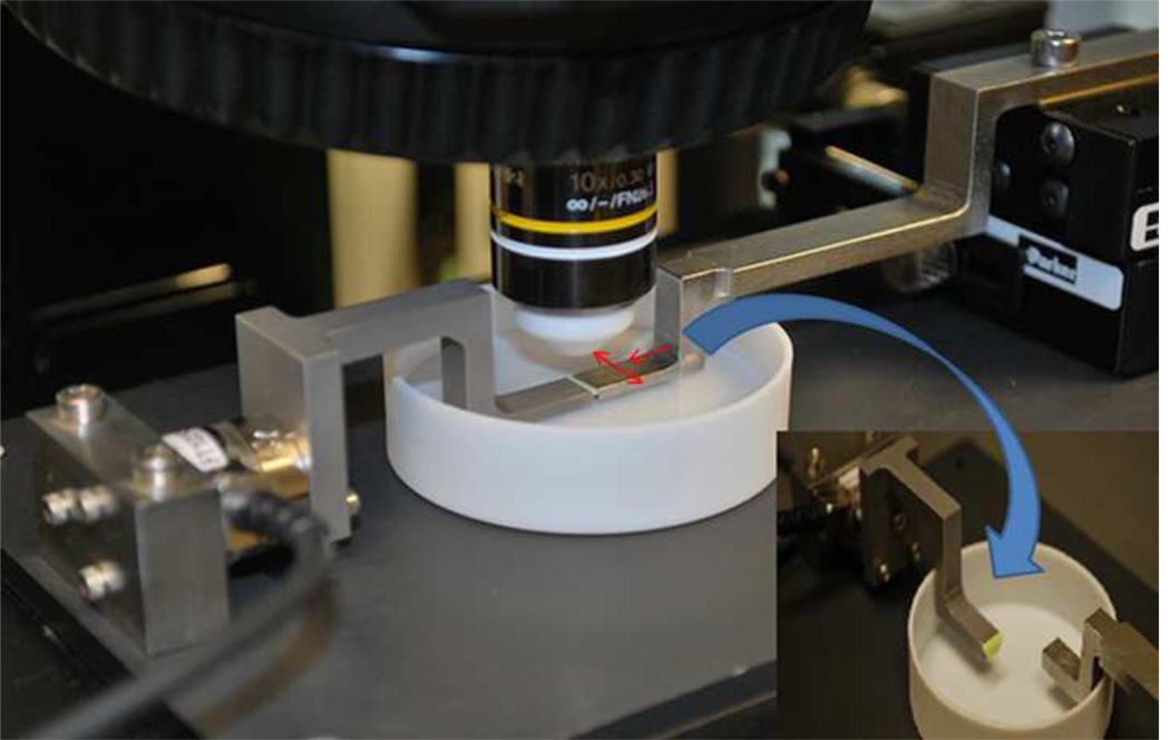
An instrument was designed to apply compressive and shear displacements to a cartilage sample while measuring shear and compressive forces (Fig. 2). During a test, the sample is immersed in PBS, while held between two stainless steel arms (Fig. 2). Since the instrument is fixed on the stage of a confocal microscope, the arms were designed so that they would not block the optical path of the microscope objective lens. Rigidity was important to maintain parallelism of the sample faces during sample deformation. Shear and compressive displacements are applied using two positioning stages (M4004-DM, Parker, Cleveland, OH) that were stacked on top of each other. One of the arms is secured to the positioning stages and the other is attached to a 6 degree of freedom load cell (Nano 17, ATI Industrial automation, Apex, NC), which has minimum resolution of 1/320 N, in both shear and compression.

Fig. 2. Apparatus.

The apparatus was designed to apply shear and compression to samples, while secured to the stage of a confocal microscope. Red arrows show applied compression and shear. The inset shows the sample attached to just one of the two arms. During the experiment, the cartilage is attached to both arms.

Samples are adhered to the arms using cyanoacrylate. Four brands of cyanoacrylate were evaluated. For three of the adhesives it appeared that the sample was separating from the stainless steel arms when immersed in PBS. The best match for our purpose was ISO-10993 Biological Tested Instant Adhesive (4011, Loctite Corp., Rocky Hill, CT).

The sample is fixed between the arms of the instrument with zero compressive strain. The apparatus is then secured on the stage of the confocal microscope. Incremental shear deflection steps (20 µm) are applied and held for two minutes, which allowed the shear force to relax. At the end of each step, an image is taken.

2.5. Imaging Technique

To determine depth-dependent mechanical behavior, we apply a previously used novel technique (Bruehlmann et al., 2004; Buckley et al., 2010) that tracks photobleached lines across the thickness of a sample. Hence, it enables qualitative and quantitative visualization of the depth-dependent shear deflection of the sample through its thickness. Displacement of photobleached lines through the thickness of the sample is obtained using an upright confocal microscope (FluoView FV1000, Olympus, Center Valley, PA). To maximize resolution, a water dipping objective lens with 0.3 numerical aperture, which yields a 1.8 µm pixel size in 1× zoom (UMPLFLN 10XW, Olympus, Center Valley, PA) is used. Lines are photobleached using a 405 nm wavelength laser with 100 percent power. For images, samples are rastered using a 488 nm laser, about 50–70 µm below the surface, with 30 percent power. We avoided using higher power to take images, since rastering the sample by itself causes photobleaching, and hence lessens image quality.

2.6. Image Processing and Data Analysis

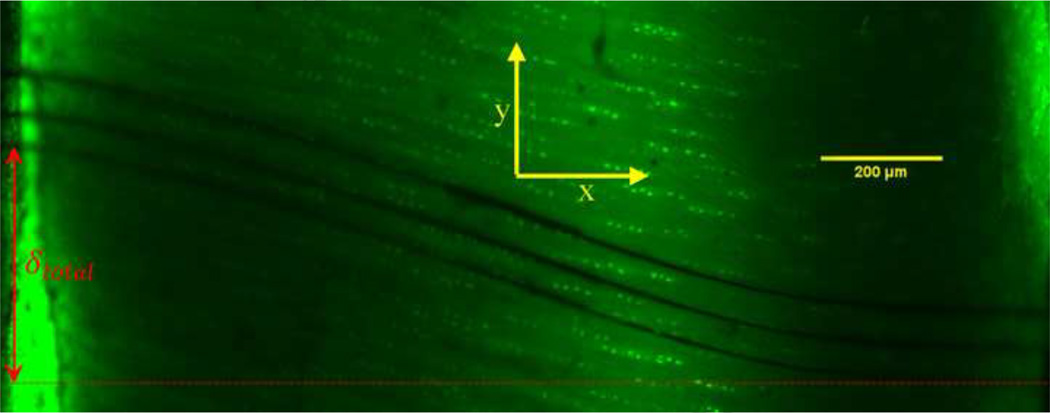
Images of photobleached lines are converted to digital values by identifying the lowest intensity pixel in every column of pixels in the y direction (Fig. 3). Numerical values associated with a photobleached line are found using a custom written MATLAB script that locates the lowest intensity pixels in every column of pixels perpendicular to the undeformed photobleached lines (x_n, y(x_n)). Three models for analytical functions (ỹ (x)) to simulate these pixel-scale discretized data are investigated: polynomials (3^rd through 9^th order), cubic splines (Harrell, 2001), and nonparametric loess (locally weighted scatter plot) curves (Cleveland, 1979). Four independent approaches are then used to identify the best-fit model.

Fig. 3. Fluorescent image of photobleached lines on native bovine AC.

Photobleached lines under shear deflection, showing the total applied shear displacement. Initially, lines were photobleached perpendicular the sample’s surface, approximately 50 to 70 µm apart. The total shear displacement was 396 µm, corresponding to a shear strain of 23%. The articular surface is on the right side and subchondral plate is on the left hand side of the image.

As our first assessment we use the Akaiki Information Criteria (AIC) (Akaiki, 1974), and the Bayesian Information Criteria (BIC) (Schwartz, 1978) to measure the relative goodness of fits. AIC and BIC are both likelihood-based model selection criteria used to judge which of a set of competing models best fits a set of data. If a model with p parameters is fit to a dataset with n observations, the AIC is defined as: AIC = −2lnL + 2p where lnL is the maximized log likelihood. Among different models, possibly non-nested and/or differing in the number of parameters p, the model with the smallest value of AIC is considered to fit the data best. By adding the term “2p” to “ −2lnL”, the AIC penalizes models with larger numbers of parameters. BIC can be written as: BIC = –2lnL + p(ln(n)). Like the AIC, the BIC penalizes models with larger numbers of parameters. For values with ln(n) > 2 (n > 7.39), the BIC criterion imposes a stricter penalty for the number of parameters as compared to the AIC. Thus, in general, use of the BIC often tends to select more parsimonious models than does use of the AIC.

In our application, the competing models are all polynomial regression models fit by least-squares regression, which is equivalent to using maximum likelihood estimation assuming normally distributed residual error terms. For a polynomial model of order k, the number of parameters is p = k + 2 (intercept + k regression coefficients + the variance of the residuals σ²). The likelihood for the i^th observation for a k^th degree polynomial model with normally distributed errors is

$$f(y_i;\theta )={(2\pi {\sigma }^2)}^{-1/2}\text{exp}[-{(y_i-{\beta }_0-{\beta }_{1}i-{\beta }_2{i}^2\dots -{\beta }_k{i}^k)}^2/(2{\sigma }^2)]$$

where θ = (β₀,β₁,β_k,σ²) is the vector of unknown parameters. The log-likelihood based on all the data, considered to be a function of θ is then defined as

$$\text{ln}L(\theta )=\text{ln}\prod _{i=1}^{n}f(y_i;\theta )=\sum _{i=1}^n\text{ln}(f(y_i;\theta ))$$

If θ̂ is the vector containing the maximum likelihood estimates of the parameters, then the maximized value of “ −2lnL” is $-2\text{ln}L(\hat{\theta })=-2\times \sum _{i=1}^n\text{ln}(f(y_i;\hat{\theta }))$. In this case, it can be shown that the negative of twice the maximized log likelihood (−2lnL) can be written in terms of the mean squared residual, where y_i and ŷ_i respectively are the observed and model-predicted predicted values of the outcome for the i^th observation. The AIC and BIC are then given by,

$$AIC=C-\frac{n}{2}\text{ln}(MSE)+2(k+2)$$

$$BIC=C-\frac{n}{2}\text{ln}(MSE)+(k+2)\text{ln}(n)$$

where C is a constant.

Additionally, we investigated the accuracy of this approach for selecting the most likely polynomial by considering a predefined curve with a shape that was similar to deflected photobleached lines. For this, we used the equation for the deflection of a beam with fixed supports, which is a third order polynomial, and added random noise to it. The appropriate level of noise was obtained by digitizing a photobleached straight line, which gave noisy pixel size data. This noise was added to the exact analytical function of the bending beam model, therefore yielding a deflected beam with the same level of noise as a processed confocal microscope image.

The second approach that was used to select a model for fitting displacement data is based a method developed to smooth and differentiate digitized data from human motion (Lesh et al., 1979). To apply this method, we use three parallel photobleached lines spaced 50 to 70 µm as depth-dependent shear deflection replicates of the same sample. The variance of the measured data is a measure of the variance of the error. The best fit minimizes the difference between variance of the error and the variance of the residual between the fitted and estimated data.

A third approach also evaluates the derivative by integrating the shear strain,×_x, across the full thickness of the sample, D

$${\delta }_{\mathit{\text{total}}}={\int }_0^D{\gamma }_{x}dx$$ (1)

where δ_total is total shear deflection, measured experimentally (Fig. 3). The integral of shear strain across the sample’s thickness is compared to the measured total shear displacement and therefore provides an additional indicator of the goodness of fit of a function to the data. We also use a custom MATLAB code to detect and calculate the total shear deflection of the sample, by averaging the three lowest intensity pixels located at each boundary (5.4 µm at right and left side of the Fig. 3) and then calculating the distance between them.

The fourth method is based on photobleaching a circular arc with a specific radius. In this case, the exact function and first derivative of the imaged curve are known, and compared with fitted values to determine their accuracy.

3. Results

We observed that photobleaching lines using a laser at 405 nm, produces sharper photobleached lines than using 492 nm which is the excitation wavelength for 5-DTAF. Consequently, the 405 nm wavelength laser with 100 percent laser power was used for photobleaching.

Before applying shear displacement, the photobleached lines appear parallel and vertical (Fig. 4A). Deformation, as imaged by the movement of photobleached lines across the thickness of tissue-engineered cartilage clearly demonstrates depth dependent variations in the stiffness of the TE cartilage (Fig. 4B). Near the outer surfaces, the lines remain nearly vertical, suggesting relatively high shear stiffness. In contrast, significant change in slope of the lines in the mid-region suggests relatively low shear stiffness. Under static shear strain of about 25%, internal failure of the cartilage is evident near the interface between the outer matrix rich region and inner matrix deficient region (Fig. 4C).

Fig. 4. Cross sections of tissue engineered cartilage stained with 5-DTAF with photobleached lines.

Before shear strains are applied, the photobleached lines appear parallel and vertical (A). Deformed photobleached lines across the thickness of tissue-engineered cartilage clearly demonstrate depth dependent variations in the stiffness of the TE cartilage (B). Under about 25% shear strain, internal failure was observed near the interface between the outer matrix rich region and inner matrix deficient region (C).

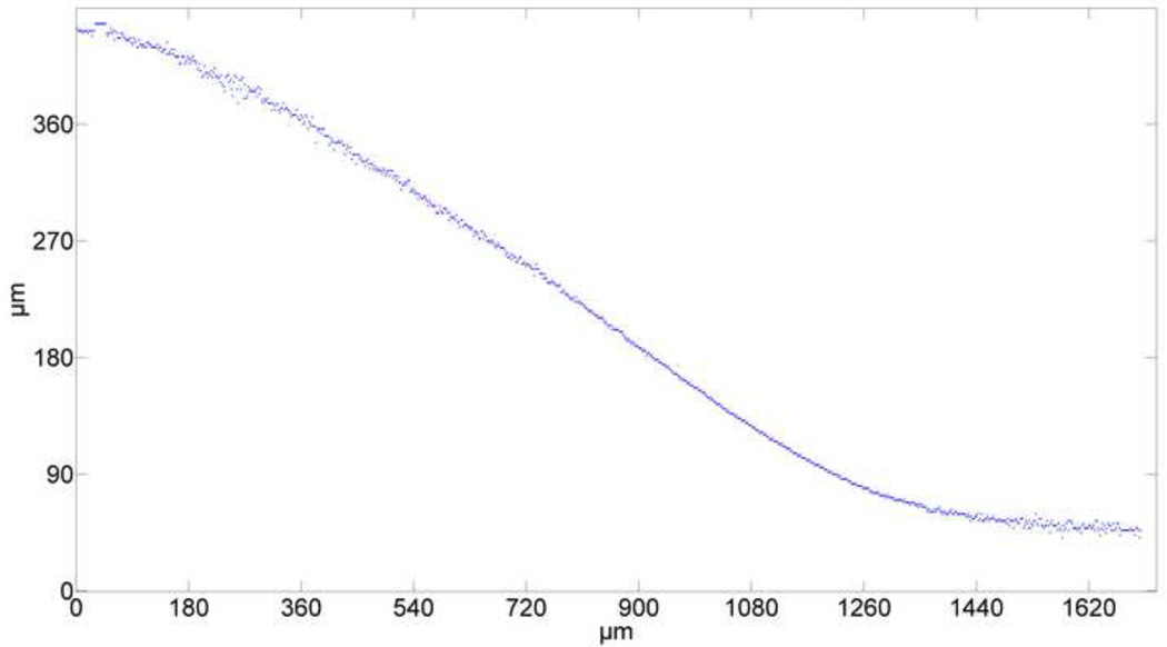
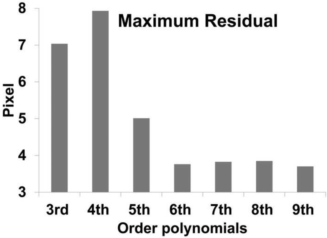
The averaged line formed from three photobleached lines on native AC consisted of 945 data points (Fig. 5). Based on both AIC and BIC, cubic splines are rejected, as they give poorer fits than polynomials models. Although nonparametric loess curves are good apparent fits to the photobleached lines, they do not yield smooth approximations of the derivatives. Both AIC and BIC give similar low values for 6^th through 9^th order polynomials, although 7^th order gives the lowest values (Table 1). Similarly, for 6^th through 9^th order polynomials the maximum residual is reduced from 8 pixels to 3.7 pixels and it remains almost constant (Fig. 6). Moreover, AIC and BIC correctly chose a third order polynomial as the most likely fit for the noisy discretized predefined deflected beam.

Fig. 5. The lowest intensity pixel averaged over three photobleached lines.

Digitized data points (pixels) represent the deflected line through the thickness of the sample. The superficial zone is on the right hand side of the graph.

Table 1.

AIC and BIC methods for different polynomials.

Order Polynomial	3rd	4th	5th	6th	7th	8th	9th
AIC	4056	4015	3664	3250	3208	3210	3211
BIC	4081	4044	3298	3289	3252	3258	3264

Fig. 6. Maximum residual of fitted polynomials from averaged digitized data.

A substantial reduction in 6^th through 9^th order polynomials was observed.

Applying the method that was developed for smoothing human motion data produced results consistent with the AIC and BIC: 6^th to 9^th order polynomials are good fits to the deformed lines (Table 2) and, comparing variances shows that differences among these polynomials are small.

Table 2.

Comparing different polynomials variance (residual variance) to error variance.

σ(yt)	3rd order σ(Rt)	4th order σ(Rt)	5th order σ(Rt)	6th order σ(Rt)	7th order σ(Rt)	8th order σ(Rt)	9th order σ(Rt)
1.6778	2.6128	2.582	2.1664	1.8201	1.805	1.7963	1.7872

However, this approach indicates that the 3^rd to 5^th order polynomials are not good fits although a 5^th order polynomial appears, visually, to be a good fit for the photobleached line (Fig. 7).

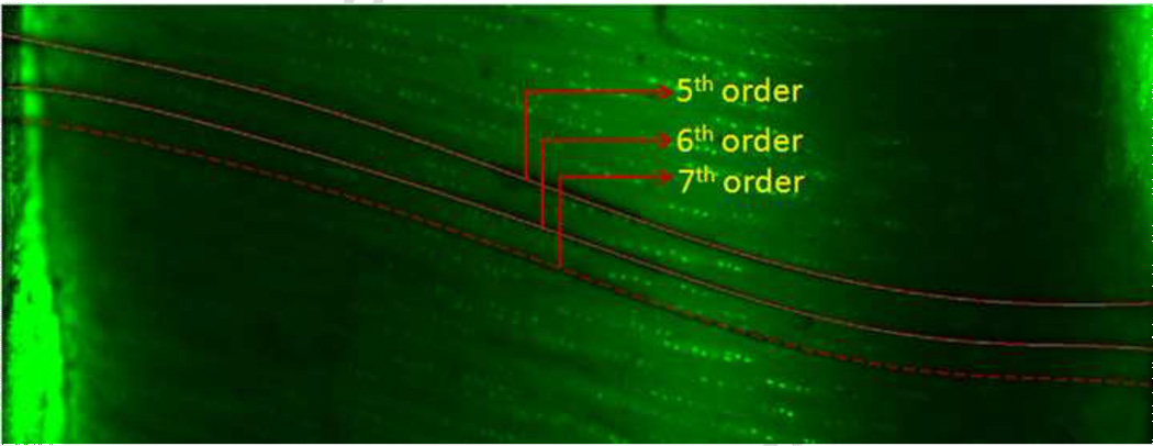
Fig. 7. Overlay of 5^th to 7^th order polynomials on deflected photobleached lines.

Three different order polynomials were fit to the deflected photobleached lines. Even though the 5^th order polynomial seems to be a good fit to the photobleached deflected line, there are significant differences in shear strain (i.e. first derivative) of 5^th and 7^th order polynomials. The articular surface is at the right side of the image.

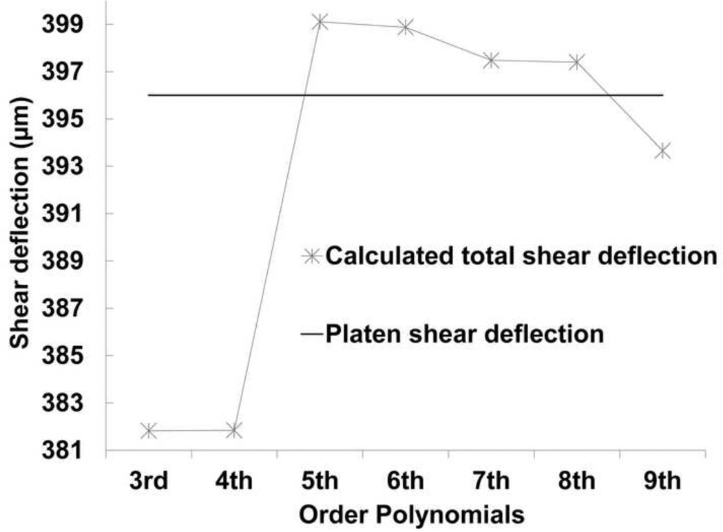
Differences between the total computed shear deflection (Eq. 1) and that measured on the sample are smallest for the 7^th, and 8^th order polynomials (Fig. 8). However, 5^th through 9^th order polynomials all give deflections that are within 3 micrometers or 0.8% of the expected value.

Fig. 8. Platen shear deflection versus calculated total shear deflection from differnet order polynomials.

Experimentally derived total shear deflection compared to calculated total shear deflection for different order polynomials. Based on this assessement 6^th to 8^th order polynomials satisfy the necessary condition to be considered as appropriate models.

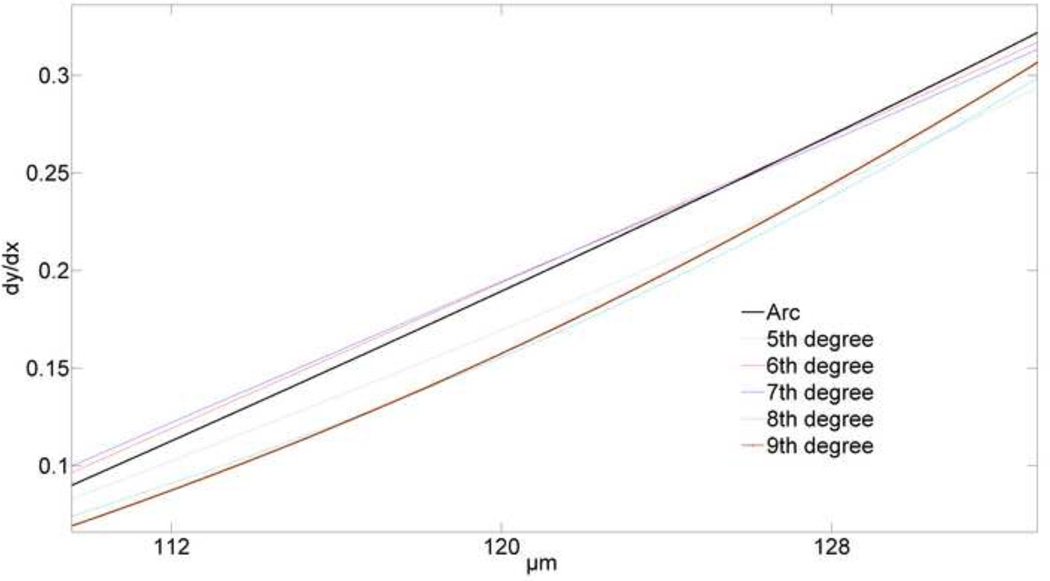
Fitting curves to sections of a circular arc showed that 6^th and 7^th order polynomials are the best overall matches to the known first derivative (Fig. 9). Near the boundaries, a 9^th order polynomial behaves poorly, and we observe that it is highly sensitive to noise, especially in this area. Comparing first derivatives shows that the 7^th order polynomial remained closer to the original curve on the boundaries, while the 6^th order polynomial fit better in the middle region of circular arc. Although there are differences between 6^th and 7^th order polynomial fits, the differences between first derivatives are less than 2%, which suggests that either could be used for our studies (Fig. 10).

Fig. 9. First derivative comparison in predefined circular region.

Close agreement of the known and analytically determined first derivatives shows that the 6^th and 7^th order polynomials are the best models to represent the circular arc.

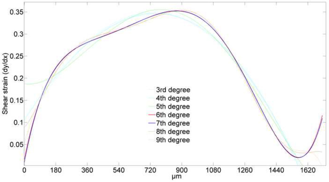
Fig. 10. First derivative of different order polynomials fit to the averaged photobleached line in AC.

Different order polynomials clearly demonstrate different first derivatives (shear strain profile), although they showed fairly similar fit to the photobleached deflected line. However, derivatives of sixth and seventh order polynomials almost coincide with each other (articular surface is on the right side).

4. Discussion

The goal of this investigation was to establish a method for finding depth dependent shear properties. This required finding the derivative of displacement data, which is an inherently noisy process. Typically, some types of data smoothing and numerical methods are used to compute derivatives. However, the level of smoothing is often arbitrary and will influence the subsequent calculation of derivatives. Here, we chose to minimize the arbitrary decisions about smoothing. First, we investigated the use of AIC and BIC for finding the best fitting curve to deflected photobleached lines as represented by pixel sized data. Based on earlier experience using low pass finite impulse response filters for smoothing and differentiating noisy data we applied that approach as an alternative (Lesh et al., 1979). Both of these approaches give us an analytical means for fitting noisy deflection data, but neither guarantees an accurate value of the derivative. Therefore, we introduced a third method that used a photobleached circle, with the same level of noise, and known first derivative to evaluate the accuracy of the derivative of our fitted curve. Finally, we introduced a fourth method that integrates the strain for comparison with the experimentally measured shear displacement. This confirmed that the model selected by the other approaches is consistent with the measured displacement data.

Although different order polynomials appear to give similar fits to the data (Fig. 7), the sensitivity of the differentiation process leads to differences in the calculated derivatives (Fig. 10). However, it is interesting to note that in our investigation, the derivatives of 6^th and 7^th order polynomials fit to the deflected photobleached lines (Fig. 10) and the circular arc (Fig. 9), almost coincide with each other. Consequently, these methods suggest that either a 6^th or 7^th order polynomial can be used to model shear displacement and strain for the native articular cartilage used in this investigation.

Taking derivatives of discrete data can introduce considerable noise. Typically, to minimize noise some type of filtering is necessary. One approach is to spatially average displacement data and then take derivatives using numerical methods that also include smoothing (Buckley et al., 2010; Buckley et al., 2008). For example, Buckley et al., used the averaged value of the displacement in 20 µm rectangular region, and applied linear methods to determine shear strain (Buckley et al., 2010). However, the level of smoothing is often arbitrary and will influence the subsequent calculation of derivatives. Technically, these methods trade off accuracy obtained from higher resolution data and obtaining less noisy results. To evaluate smoothing and numerical differentiation in relation to our curve fitting method, we first smoothed the data by averaging displacement in 1, 5, 11, and 22 pixel windows (1.8, 9, 19.8, and 39.6 µm respectively) and then computed shear strain using five-point linear least squares fitting (5PLSQ) for native AC. These windows were smaller, the same (~ 20 µm), and larger than those used in previous studies (Buckley et al., 2010). Using one-pixel windows (no smoothing) leads to substantial noise that obscures the pattern of the shear strain. We observed that the numerical results oscillated about our analytical result (Fig. 11A). As the size of the averaging window increased the derivative became smoother. However, smoothness does not guarantee accuracy of the derivative. As shown (Fig. 11A), the numerical method fairly approximates the shear strain, but the level of smoothing dominantly affects the results. A potentially deleterious effect of smoothing by averaging in a window is loss of resolution. For instance, the minima close to the superficial zone could be easily smoothed by choosing a window larger than 39.6 µm, however, this minima was observed partially by smaller averaging windows (Fig. 11A). If we are interested in the behavior of the superficial zone, which is approximately 10% of the thickness or about 170 µm, in the extreme choosing a 170 µm window would over-smooth the material behavior and probably obscure potentially valuable results such as increased shear compliance of the superficial zone due to buckling of collagen fibers under compression (Buckley et al., 2008). Even smaller windows could limit resolution. Averaging in 20 µm windows produces about eight data points. However, near the boundaries the number of points is further reduced since it is not possible to average in full-sized windows up the boundaries. Since 5PLSQ requires two windows on either side of the point where the derivative is being computed, resolution is further limited near boundaries (Fig. 11A).

Fig. 11. Comparing first derivatives using analytical and linear numerical methods.

Depth dependent shear strain in native AC computed from the derivative of a 7^th order polynomial, and numerical 5PLSQ proceeded by averaging displacements in 9, 19.8, and 39.6 µm windows. As the window size is increased, the numerical derivative becomes smoother and approaches the 7^th order polynomial. Note that as the window size is increased, the size of the region near the boundaries where the derivative cannot be computed also increases. The articular surface is on the right side of the plot (A). Known first derivative (slope) of a beam with fixed supports, and numerical 5PLSQ preceded by averaging displacements in 9, 19.8, and 39.6 µm windows. In general, the numerical results are smoother and closer to the known function for the larger window (B).

Using the deflected beam function with noise gives us an added opportunity to compare numerical derivatives to the known value, and to evaluate the effect of smoothing by varying the window size. This comparison showed that the derivative computed using larger averaging windows generally converged to the true function (Fig. 11B). However, in some areas the smaller windows predicted the first derivate more accurately. We expect that these inconsistencies might be due to the noise level, since we observed that noise level of the original data influences the numerical differentiation results, which is an inherent problem for numerical differentiation. Therefore, implementing unvalidated arbitrary numerical smoothing methods could compromise the accuracy of the results, especially near boundaries.

As a result, the lack of a validated method to predict the depth-dependent properties prompted us to establish a systematic method that has been validated mathematically and experimentally. Although validated, it is possible that this method could, like numerical methods, attenuate smallscale variations in material properties. However, without the reduction in the number of data points that results from using averaging, a local variation in material properties might be more easily captured by a piecewise polynomial fit of all of the data in a localized region. Although 6th and 7^th order polynomials were shown to be the best models for the full tissue thickness, it is possible that for other tissues different order polynomials would be the best fit, or that piecewise fits may be needed in the case of discontinuities. Since the AIC and BIC methods are easily implemented and showed excellent agreement with the other methods used in this investigation, extending this approach to other tissues is feasible.

The utility of this image-based approach for qualitative evaluation of TE cartilage was also demonstrated. Applying this method to TE cartilage clarifies previous work that suggested that failure under static compression and cyclic shear occurs in the matrix deficient region in the middle layer of TE cartilage (Whitney et al., 2010a). We observed crack initiation near the interface between the outer matrix rich region and inner matrix deficient region of TE cartilage. This approach can be helpful for assessing quantitative and qualitative variations in tissue produced under different culture conditions.

In summary, we have developed and validated a method for determining pixel level shear displacement, and noiseless estimates of shear strain. The motivation for this work is the mechanical evaluation of tissue-engineered cartilage. As shown here, it is possible to determine quantitative estimates of shear modulus as well as qualitative insights into tissue failure.

References

- Akaiki H. A New Look at the Statistical Model Identification. IEEE Trans Automat Contr. 1974;19:716–723. [Google Scholar]
- Benchaib M, Delorme R, Pluvinage M, Bryon PA, Souchier C. Evaluation of five green fluorescence emitting streptavidin conjugated fluorochromes for use in immunofluorescence microscopy. Histochem Cell Biol. 1996;106:253–256. doi: 10.1007/BF02484409. [DOI] [PubMed] [Google Scholar]
- Bruehlmann SB, Matyas JR, Duncan NA. Collagen Fibril Sliding Governs Cell Mechanics in the Anulus Fibrosus. J Spine. 2004;29:2612–2620. doi: 10.1097/01.brs.0000146465.05972.56. [DOI] [PubMed] [Google Scholar]
- Buckley MR, Bergou AJ, Fouchard J, Bonassar LJ, Cohen I. High resolution spatial mapping of shear properties in cartilage. J Biomech. 2010;43:796–800. doi: 10.1016/j.jbiomech.2009.10.012. [DOI] [PMC free article] [PubMed] [Google Scholar]
- Buckley MR, Gleghorn JP, Bonassar LJ, Cohen I. Mapping the depth dependence of shear properties in articular cartilage. J Biomech. 2008;41:2430–2437. doi: 10.1016/j.jbiomech.2008.05.021. [DOI] [PubMed] [Google Scholar]
- Buckwalter JA, Mankin HJ. Instructional Course Lectures, The American Academy of Orthopaedic Surgeons – Articular Cartilage. Part I: Tissue Design and Chondrocyte Matrix Interactions. J Bone Joint Surg. 1997;70-A:600–611. [Google Scholar]
- Canal CE, Hung CT, Ateshian GA. Two dimensional strain fields on the cross section of the bovine humeral head under contact loading. J Biomech. 2008;41:3145–3151. doi: 10.1016/j.jbiomech.2008.08.031. [DOI] [PMC free article] [PubMed] [Google Scholar]
- Chen AC, Bae WC, Schinagl RM, Sah RL. Depth and strain dependent mechanical and electromechanical properties of full thickness bovine articular cartilage in confned compression. Journal of Biomechanics. 2001;34:1–12. doi: 10.1016/s0021-9290(00)00170-6. [DOI] [PubMed] [Google Scholar]
- Cleveland WS. Robust Locally Weighted Regression and Smoothing Scatterplots. Stat Biopharm Res. 1979;74:829–836. [Google Scholar]
- Harrell F. Regression Modeling Strategies with Applications to Linear Models, Logistic Regression, and Survival Analysis. Springer Verlag; 2001. p. 20. [Google Scholar]
- Hosoda N, Sakai N, Sawae Y, Murakami T. Depth Dependence and Time Dependence in Mechanical Behaviors of Articular Cartilage in Unconfined Compression Test under Constant Total Deformation. JBSE. 2008;3:209–220. [Google Scholar]
- Hunziker EB, Kapfinger E, Geiss J. The structural architecture of adult mammalian articular cartilage evolves by a synchronized process of tissue resorption and neoformation during postnatal development. Osteoarthritis Cartilage. 2007;15:403–413. doi: 10.1016/j.joca.2006.09.010. [DOI] [PubMed] [Google Scholar]
- Jayaraman K. Mechanical and Aerospace Engineering. Case Western Reserve University; 2010. DAMAGE AND WEAR OF NATIVE AND TISSUE ENGINEERED CARTILAGE; p. 126. [Google Scholar]
- Lesh MD, Mansour JM, Simon SR. A Gait Analysis Subsystem for Smoothing and Differentiation of Human Motion Data. J Biomech Eng. 1979;101:205–212. [Google Scholar]
- Lopez O, Amrami KK, Manduca A, Ehman RL. Characterization of the Dynamic Shear Properties of Hyaline Cartilage Using High Frequency Dynamic MR Elastography. Magnetic Resonance in Medicine. 2008;59:356–364. doi: 10.1002/mrm.21474. [DOI] [PubMed] [Google Scholar]
- Pezzack JC, Norman RW, Winter DA. An Assessment of Derivative Determining Techniques Used for Motion Analysis. Journal of Biomechanics. 1977;10:377–382. doi: 10.1016/0021-9290(77)90010-0. [DOI] [PubMed] [Google Scholar]
- Schinagl RM, Gurskis D, Chen AC, Sah RL. Depth Dependent Confined Compression Modulus of Full Thickness Bovine Articular Cartilage. Journal of Orthopaedic Research. 1997;15:499–506. doi: 10.1002/jor.1100150404. [DOI] [PubMed] [Google Scholar]
- Schwartz G. Estimating the Dimension of A Model. Ann Stat. 1978;6:461–464. [Google Scholar]
- Weidenbecher M, Tucker HM, Wadallah A, Dennis JE. Fabrication of a neotrachea using engineered cartilage. Laryngoscope. 2008;118:593–601. doi: 10.1097/MLG.0b013e318161f9f8. [DOI] [PMC free article] [PubMed] [Google Scholar]
- Whitney GA, Jayaraman K, Dennis JE, Mansour JM. Biomedical Engineering Society Annual Meeting. Austin, Texas: 2010a. Highly cellular region of scaffold free engineered cartilage fails under compressive shearing loads. [Google Scholar]
- Whitney GA, Jayaraman K, Mansour JM, Dennis JE. TERMIS-NA. Orlando, Florida: 2010b. Assessment and improvement of scaffold free engineered articular cartilage mechanical function. [Google Scholar]
- Whitney GA, Mansour JM, Dennis JE. ORS Annual Meeting. San Francisco: 2012a. Improved function of scaffold free engineered cartilage under combined compressive and shear loads. [Google Scholar]
- Whitney GA, Mera H, Weidenbecher M, Awadallah A, Mansour JM, Dennis JE. Methods for Producing Scaffold Free Engineered Cartilage Sheets from Auricular and Articular Chondrocyte Cell Sources and Attachment to Porous Tantalum. Biores Open Access. 2012b;1:157–165. doi: 10.1089/biores.2012.0231. [DOI] [PMC free article] [PubMed] [Google Scholar]
- Winter DA, Sidwall HG, Hobson DA. Measurement and Reduction of Noise in Kinematics of Locomotion. Journal of Biomechanics. 1974;7:157–159. doi: 10.1016/0021-9290(74)90056-6. [DOI] [PubMed] [Google Scholar]
- Wong BL, Bae WC, Chun J, Gratz KR, Lotz M, Sah RL. Biomechanics of Cartilage Articulation: Effects of Lubrication and Degeneration on Shear Deformation. Arthritis Rheum. 2008a;58:2065–2074. doi: 10.1002/art.23548. [DOI] [PubMed] [Google Scholar]
- Wong BL, Bae WC, Gratz KR, Sah RL. Shear Deformation Kinematics During Cartilage Articulation: Effect of Lubrication, Degeneration, and Stress Relaxation. Mol Cell Biomech. 2008b;5:197–206. [PMC free article] [PubMed] [Google Scholar]
- Wong BL, Sah RL. Mechanical asymmetry during articulation of tibial and femoral cartilages: Local and overall compressive and shear deformation and properties. Journal of Biomechanics. 2010;43:1689–1695. doi: 10.1016/j.jbiomech.2010.02.035. [DOI] [PMC free article] [PubMed] [Google Scholar]