A general approach for discriminative de novo motif discovery from high-throughput data

Abstract

De novo motif discovery has been an important challenge of bioinformatics for the past two decades. Since the emergence of high-throughput techniques like ChIP-seq, ChIP-exo and protein-binding microarrays (PBMs), the focus of de novo motif discovery has shifted to runtime and accuracy on large data sets. For this purpose, specialized algorithms have been designed for discovering motifs in ChIP-seq or PBM data. However, none of the existing approaches work perfectly for all three high-throughput techniques. In this article, we propose Dimont, a general approach for fast and accurate de novo motif discovery from high-throughput data. We demonstrate that Dimont yields a higher number of correct motifs from ChIP-seq data than any of the specialized approaches and achieves a higher accuracy for predicting PBM intensities from probe sequence than any of the approaches specifically designed for that purpose. Dimont also reports the expected motifs for several ChIP-exo data sets. Investigating differences between in vitro and in vivo binding, we find that for most transcription factors, the motifs discovered by Dimont are in good accordance between techniques, but we also find notable exceptions. We also observe that modeling intra-motif dependencies may increase accuracy, which indicates that more complex motif models are a worthwhile field of research.

INTRODUCTION

New high-throughput techniques such as ChIP-seq (1), ChIP-exo (2) and protein-binding microarrays (PBMs) (3) have dramatically increased the amount and quality of data that can be used for de novo motif discovery. ChIP-seq experiments determine binding regions of DNA-binding proteins in vivo by cross-linking protein and DNA, immunoprecipitating the targeted protein and sequencing the bound fragments. In case of ChIP-exo, the fragments are shortened by an exonuclease before sequencing. PBMs allow for measuring probe-specific binding affinity in vitro for a huge number of systematically chosen double-stranded probes. Despite the experimental differences, these approaches yield thousands of candidate binding regions together with a measure of confidence, which can be used for de novo motif discovery.

Ma et al. (4) provide an extensive comparison of de novo motif discovery tools capable of using ChIP-seq data, where ChIPMunk (5) and POSMO (4) are the best-performing tools closely followed by DME (6), DREME (7) and MEME (8). A detailed comparison of de novo motif discovery tools using PBM data is given by Weirauch et al. (9), where FeatureREDUCE emerges as top-performing algorithm. However, there is no tool that works well for data from both experimental techniques (9). For ChIP-exo data, no specialized tool is currently available, and research resorts to well-established algorithms from the pre-NGS era (2).

The lack of a universally applicable approach hampers the integration of data from different techniques and complicates the comparison of the resulting motifs, e.g. between in vivo and in vitro binding. Hence, we propose Dimont, a general approach for probabilistic discriminative de novo motif discovery that is capable of handling ChIP-seq, ChIP-exo and PBM data.

The runtime of most probabilistic de novo motif discovery tools is mainly determined by iteratively evaluating the likelihood. As the positions of the binding sites within the target sequences are unknown (hidden variables), these tools need to consider all admissible binding site positions for evaluating the likelihood, which has a decisive influence on runtime. One approach to circumvent this problem is to resort to k-mer enumeration methods like POSMO (4), which yields a competitive runtime even on large data sets. Dimont implements an alternative approach that allows for adhering to probabilistic methods using the popular ‘zero or one occurrence per sequence’ (ZOOPS) model of many de novo motif discovery tools (8,10–13) while achieving acceptable runtimes. Dimont uses that only a few binding sites are buried within long target sequences. In most probabilistic approaches, this results in a big discrepancy between the number of finally predicted binding sites and the number of positions that need to be evaluated for computing the likelihood, and in wasting a considerable amount of runtime during training.

Hence, we only consider those positions contributing the most to the likelihood of a target sequence (Figure 1). During optimization, we dynamically determine the positions to be evaluated keeping the learning scheme flexible to adapt to the positions of potential binding sites. This acceleration scheme allows for using all ChIP binding regions or all PBM probe sequences for de novo motif discovery instead of limiting the input data to a fixed number of (high-confidence) sequences (14).

Figure 1.

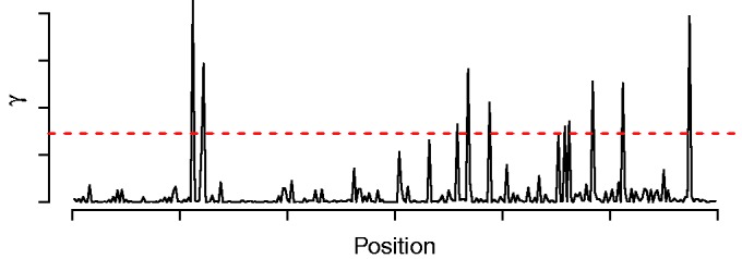
Normalized likelihood profile of a sequence. The red dashed line visualizes the threshold that is used to accelerate the algorithm. All positions with peaks above the threshold are included in , and all remaining positions are not used for evaluating the likelihood.

As peak occupancies or probe intensities contain valuable information for motif discovery, Dimont converts these to soft labels reflecting the a priori probability of a sequence being bound. These soft labels are used for learning parameters by a weighted variant (15) of the discriminative maximum supervised posterior principle (16,17).

In previous studies, the complexity of motif models was limited mostly owing to the limited amount of data. For this reason, simple models including consensus sequences as well as position weight matrices and sequence logos as their graphical representation are widespread. However, due to the enormous amount of high-throughput data, more complex models including inhomogeneous Markov models of higher order, which have been proven advantageous for other binding sites (18,19), can be used for de novo motif discovery and prediction of transcription factor binding sites. Hence, we include the capability of learning higher-order inhomogeneous Markov models into Dimont.

We implement Dimont within the open-source Java library Jstacs (20). We provide a Dimont web server at http://galaxy.informatik.uni-halle.de and a stand-alone command line application at http://www.jstacs.de/index.php/Dimont.

MATERIALS AND METHODS

The input data of Dimont are DNA sequences where each symbol is from the DNA alphabet . Each of the sequences is assigned some measure of evidence that reflects how likely this sequence is bound by the transcription factor of interest. In case of ChIP-seq and ChIP-exo data, such a measure is the number of reads or fragments under a ChIP peak, often termed ‘peak statistic’ or ‘peak occupancy’. For PBM data, such a measure is the signal intensity of the probe sequence on the microarray.

In the following, we assume that high-confidence sequences, i.e. those with a high peak statistic or a high signal intensity, contain a binding site of the motif of interest with substantially higher probability than low-confidence sequences. Hence, we transform these measures to probabilities that reflect how likely a sequence is bound by the transcription factor as explained in ‘Soft labels from peak statistics and signal intensities’ section. For ChIP-seq and ChIP-exo data, we additionally assume that binding sites of the targeted transcription factor occur clustered around the centers of the ChIP peaks. Hence, we use a non-uniform position distribution over the binding site positions in the Dimont model, which we introduce in ‘Dimont models and objective function’. In subsequent sections, we describe how we accelerate the optimization of the parameters of the Dimont model, we outline the complete Dimont algorithm, and we introduce the performance measures and data sets used in the case studies of this article.

Soft labels from peak statistics and signal intensities

We map the peak statistics of ChIP data and the signal intensities of PBM data to soft labels that reflect the probability assumed a priori of being bound by the targeted factor. For this reason, we refer to the probabilty of being bound as ‘foreground probability’ and to the converse probability as ‘background probability’.

Here, we propose a mapping that is based on the ranks of the signals within a data set. We denote as r_n the rank of the n-th sequence in the data set. Let be the maximum rank, and let be the relative rank. We set q to the a priori fraction of sequences that receives a foreground probability greater than 0.5, and we refer to q as ‘weighting factor’. The value of q can be adapted to the characteristics of the data, for instance, the significance level of accepted ChIP-seq peaks. In general, it is reasonable for any data source to also include low-confidence sequences into the input data to preserve the discriminative nature of Dimont. In our studies, we use for ChIP data and for PBM data. We define the foreground probability of sequence as

(1)

and the background probability as . For simplicity reasons, we refer to the sequences in conjunction with the foreground probability as ‘foreground’ and to the same sequences in conjunction with the background probability as ‘background’.

Dimont models and objective function

Dimont is based on the popular ZOOPS model used in many de novo motif discovery tools (8,10–13). In Dimont, the motif model is a uniform mixture model over the DNA strands using an inhomogeneous Markov model of user-specified order, which includes the position weight matrix (PWM) model (21,22) for order 0 and the weight array matrix model (18,19) for order 1. We give a detailed definition of the likelihood of the motif model in Section 1 of the Supplementary Material.

In addition, we use a non-uniform position distribution over all possible binding site positions relative to an anchor position. More specifically, we use a Gaussian distribution with given initial standard deviation of 75 around the anchor position for ChIP-seq, ChIP-exo and PBM data (details in Section 2 of the Supplementary Material).

For positions not covered by a binding site, we use a uniform distribution. Hence, the likelihood of an input sequence , given the ZOOPS model with parameters is defined as

(2)

where denotes the a priori probability of observing a motif in a sequence, is the set of admissible positions, initially set to , and denotes the likelihood of the motif model of width w. During optimization, we adapt according to the acceleration scheme described in Accelerated discriminative learning section.

As background model , we use either a uniform distribution or a homogeneous Markov model of order d.

To optimize the parameters of these models, we introduce a weighted variant (15) of the discriminative maximum supervised posterior principle (17,16,23) to de novo motif discovery, i.e.

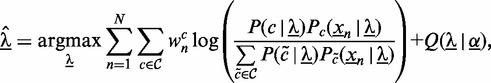(3)

where is the set of classes, and denotes the prior on the parameters given hyper-parameters . In case of Dimont, this prior is a transformed product-Dirichlet prior (23) using BDeu hyper-parameters (24,25) based on an equivalent sample size of 4 for the foreground class and for the background class. Parameter optimization is performed numerically using conjugate gradients.

Accelerated discriminative learning

We achieve an acceleration of parameter optimization by two general ideas. First, we perform a pre-optimization of parameters using a ‘reduced data set’ containing the highest-confidence sequences of foreground and background class (Hence, these sequences also correspond to the lowest-confidence sequences of the alternative class). To this end, we select the 30% of the sequences, but not >1000 sequences in total, obtaining the most extreme probabilities and , respectively. We select these sequences such that the proportion of foreground and background probabilities is approximately identical to the full data set by successively adding sequences with the highest and , respectively.

Second, we observe that only few binding sites are detected within long target sequences as exemplarily depicted in Figure 1. A large proportion of runtime is wasted while evaluating the likelihood of the motif model for positions that will never be predicted as potential binding sites. Hence, we only use the most relevant positions corresponding to the largest summands in Equation (2) instead of computing all terms. For this reason, we compute and normalize all summands of Equation (2) for each sequence yielding

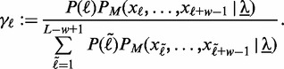(4)

We then rank the positions by in descending order. This rank is different from the rank r_n according to the peak statistics or signal intensities, respectively, as given by the biological experiment. Here, the rank reflects the prediction due to the statistical model. Subsequently, we select in descending order a set of relevant positions until 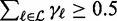, and we refer to this threshold as ‘likelihood cutoff’. During numerical optimization, we determine at the beginning of each iteration using the current set of parameters . Evaluating the likelihood of Equation (2) in the numerical optimization, we only use the positions in .

The Dimont algorithm

In the following, we describe the Dimont algorithm step by step.

Pre-processing

We read the input sequences including peak statistics or probe intensities, which we convert to soft labels.

Initialization

For initializing the motif model, we first enumerate all 7mers that occur in the reduced data set. We then rank these 7mers by 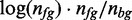, where n_fg is the sum of the foreground probabilities of all sequences containing the current 7mer at least once, and n_bg is the corresponding sum of the background probabilities . We filter the ranked 7mers by excluding redundant variants, which have a Hamming distance of <2 to better-ranked 7mers.

Of the ranked and filtered 7mers, we select the top 50 7mers and use each of these to initialize the core of a motif model of initial width w such that the central positions obtain a probability of 0.9 for the corresponding nucleotide in the 7mer and a probability of for the remaining nucleotides. The bordering positions are assigned a uniform distribution. We then evaluate the conditional likelihood, i.e. Equation (3) without the prior term, and choose the top m initial motifs with respect to conditional likelihood.

Pre-optimization

For each of the m initial motifs, we optimize the parameters according to Equation (3) on the reduced data set using the accelerated optimization described in the previous section. We then rank the resulting motifs by the supervised posterior achieved in the optimization.

Filtering motifs

Initialization and pre-optimization may result in redundant motifs, e.g. shifted variants or reverse complementary motifs. To reduce runtime, we filter such redundant motifs before the final optimization. We consider two motifs redundant if their score profiles, i.e. their for all positions show a Pearson correlation greater than 0.3, averaged over all sequences in the reduced data set. During this filtering step, we allow for shifts of the score profiles up to w in both directions. If two motifs are considered redundant, we keep the motif variant achieving the larger supervised posterior.

Final optimization

For each of those motifs that remain after the filtering step, we optimize the parameters with respect to Equation (3) on the complete input data set. Subsequently, we compute the Kullback–Leibler divergence (26) between the marginal distribution at each motif position and the nucleotide composition of the complete data set. We remove bordering motif positions as long as Kullback–Leibler divergence is below 0.2. If Kullback–Leibler divergence exceeds 0.8 for a bordering position, we expand the motif by one additional position. We then adjust the standard deviation of the position distribution, and finally optimize the parameters with respect to Equation (3) on the complete input data set. Again, we rank the resulting motifs by the supervised posterior achieved in the optimization on the complete data set.

Post filtering

We finish the Dimont algorithm with a final filtering step in analogy to pre-optimization to eliminate redundantly reported motifs.

Default parameters

As default parameters of Dimont, we suggest (i) a motif model of order of 0, i.e. a PWM model; (ii) a uniform background model; (iii) a weighting factor of ; (iv) an initial motif width of w = 15; and (v) m = 20 pre-optmization runs. We use these default parameters throughout this article if not stated otherwise.

Performance measures

For evaluating the performance of de novo motif discovery predictions, several measures have been used. For PBM data, we stick to the area under the receiver-operating characteristic curve (AUC-ROC) and Pearson correlation, as these have been used as final performance measures in the DREAM5 challenge (9). Pearson correlation is sensitive to monotone transformations of the predicted scores, while AUC-ROC is insensitive to such transformations. For maximizing the Pearson correlation, we search an adequate transformation,

(5)

where r is the predicted score, namely, the likelihood ratio, and c is a free parameter. We optimize c to maximze the Pearson correlation on the training data and use this optimal value to transform the likelihood ratios of the test data. For computing AUC-ROC, probe sequences with a mean signal intensity >4 standard deviations above the experiment average are assigned to the positive class, and all other probe sequences are assigned to the negative class (9).

Comparing the results of Dimont to other tools and between experiments, we use sequence logos as proposed by Ma et al. (4), the normalized Euclidean distance as proposed by Linhart et al. (27) and AUC-ROC.

Data

ChIP-seq data

We obtain the ChIP-seq peaks (centers and peak statistics) of the 26 ChIP-seq data sets compiled by Ma et al. (4) from original publications (28–34). For the comparison of ChIP-seq and PBM data, we additionally obtain the ChIP-seq peaks of Foxo1 (GSM546525, (35)), GATA4 (GSM558904, (36)), Tcf3 (GSM915177, unpublished) Tbx5 (GSM558908, (36)) and Tbx20 (GSM734426, (36)) from Gene Expression Omnibus (http://www.ncbi.nlm.nih.gov/geo/), and of Nr5a2 (SRP001796, (37)) from the hmChIP database ((38), http://jilab.biostat.jhsph.edu/database/cgi-bin/hmChIP.pl).

For each of these data sets, we download the genome sequences of the corresponding species and genome version (hg18, mm8, mm9, dm3) from the UCSC Genome Browser (http://hgdownload.cse.ucsc.edu/downloads.html). For each ChIP-seq peak, we extract 1000 bp of genomic sequence centered around the given peak summit and annotate these sequences with the corresponding peak statistic.

ChIP-exo data

We obtain the ChIP-exo peaks (peak coordinate and occupancy) from the supplement of Rhee and Pugh (2). For CTCF, we download the human genome sequences (hg18) from the UCSC Genome Browser. In case of the three yeast data sets, we obtain the yeast genome (build 19-Jan-2007) from the Saccharomyces Genome Database (http://www.yeastgenome.org/download-data). For each ChIP-exo peak, we extract, based on CW distance, 200 bp (CTCF) or 100 bp (yeast factors) of genomic sequence centered around the given peak center, and we annotate these sequences with the corresponding peak occupancy.

PBM data

We obtain the 40 tuning, the 66 training and the 66 test PBM data sets of DREAM5 challenge2 (http://wiki.c2b2.columbia.edu/dream/index.php/D5c2). For the comparison of ChIP-exo and PBM data, we additionally obtain PBM data sets for Phd1 (UP00351) and Rap1 (UP00321) from the UniPROBE database (39,40) (http://thebrain.bwh.harvard.edu/uniprobe/). Of each probe sequence, we extract the first 40 bp, comprising 35 unique base pairs and 5 bp of linker sequence.

In case of the PBM data sets of DREAM5, we follow the proposal of Weirauch et al. (9) and use the mean signal intensities after spatial detrending and quantile normalization.

RESULTS

Runtime

We assess the runtime of Dimont on all data sets considered in this article on a standard laptop (Intel Core i7, ULV, dual core, 2 Ghz) using standard parameters. In Figure 2, we plot the runtime of Dimont against the size of the input data set for different types of input data. For ChIP-seq data sets comprising sequences of length 1000 bp, we observe runtimes of ∼5 min for medium sized data sets. On the largest ChIP-seq data set containing 73 795 sequences of length 1000 bp, Dimont runs for 1 h 15 min. Without the speed-up strategy described in Accelerated discriminative learning section, runtime would increase by a factor of 5 to 29 as shown for selected data sets, namely, KNI (504 sequences), c-Myc (3 413 sequences), KR2 (5 793 sequences) and FoxA2 (11 461 sequences). We give a detailed overview of runtime dependency on the speed-up strategy and motif order in Supplementary Figures S1–S3.

Figure 2.

Runtime evaluation of Dimont on the data sets used in this article. We consider all ChIP-seq data sets (blue), ChIP-exo (red) and PBM (green) data sets used in this article. Upright triangles represent the runtime without the speed-up strategy, whereas reversed triangles represent the runtime using the speed-up strategy. Runtime decreases by a factor of 5 to 29 due to the speed-up strategy.

For ChIP-exo data sets comprising sequences of length 200 in case of CTCF and sequences of length 100 in case of the yeast data sets, runtime decreases substantially, and Dimont reports a motif after at most 5 min.

In case of the PBM data containing ∼40 000 probe sequences of length 40 bp per data set, Dimont runs for 2–8 min.

ChIP-seq

In a first case study, we assess Dimont using default parameters on the 26 ChIP-seq data sets of Ma et al. (4). In Figure 3, we present exemplary motifs for three of the factors considered, while the motifs reported for all data sets are available in Supplementary Figure S4. In addition to a visual comparison of the motifs discovered to those from the literature, we consider the normalized Euclidean distance (27) between the two motifs as a measure for their similarity.

Figure 3.

Three exemplary motifs discovered by Dimont on the FoxA2, Tcfcp2l1 and KNI data sets of Ma et al. (4) compared with the corresponding motifs from the Jaspar database.

The motif of FoxA2 discovered by Dimont closely resembles the motif reported in the Jaspar database (41) with clear consensus GTAAACA (normalized Euclidean distance ). The motif of Tcfcp2l1 is also recovered well by Dimont (), although minor differences are visible: the strength of conservation at some positions differs between the motif reported by Dimont and that of Jaspar. In addition, Dimont includes two additional positions with a slight preference for A into the motif, while the last conserved G, present in the Jaspar motif, is omitted. The latter might be an effect of the strand model of Dimont combined with the roughly palindromic structure of Tcfcp2l1.

The motif of KNI () is one of three motifs that are discovered from ChIP-seq data exclusively by Dimont (c.f. Supplementary Figure S4, Table 1). We find that the consensus of the Jaspar motif (AAANTAGAGCA) fits the motif discovered by Dimont. However, we find two notable differences between the two motifs. First, the sequence of As at the 5′ end of the motif is more conserved in the Jaspar motif. Second, we find mildly conserved Gs at positions 4 and 12 of the motif reported by Dimont, which are not present in the Jaspar motif.

Table 1.

Number of motifs successfully discovered by Dimont on the data sets compiled by Ma et al. (4) compared with the results of POSMO, ChIPMunk, MEME, DME, DREME and HMS

Algorithm	Total successes	Average rank
Dimont	26	1.23
POSMO	23	1.00
ChIPMunk	23	1.00
MEME	22	1.32
DME	22	1.45
DREME	22	1.45
HMS	12	1.00

We define a discovery successful iff the normalized Euclidean distance between the predicted motif and the motif described in the literature is smaller than 0.25.

We assess the performance of Dimont on all data sets of Ma et al. (4) by counting the number data sets for which Dimont successfully discovers the known motif for the targeted transcription factor. We define a discovery successful iff the normalized Euclidean distance between the predicted motif and the motif described in the literature (4,33,34,41,42) is smaller than 0.25. We give an overview of this assessment in Table 1, and we additionally include the number of motifs correctly discovered by POSMO (4), MEME (8), DME (6), ChIPMunk (5), HMS (42) and DREME (7) as reported by Ma et al. (4). All motifs discovered by Dimont are presented in Supplementary Figure S4.

We find by comparing the discovered motifs to the literature using the normalized Euclidean distance that Dimont discovers all 26 motifs. As reported by Ma et al. (4), POSMO and ChIPMunk discover 23 motifs; MEME, DME and DREME discover 22 motifs; and HMS discovers 12 motifs. Three motifs (CAD, E2f1 and KNI) are discovered only by Dimont but by none of the previous approaches.

Considering the average rank of correct predictions, we find that for 20 of the 26 data sets, Dimont reports the correct motif on rank 1. For the remaining six data sets (CAD, GT, KNI, KR1, KR2 and Nanog), Dimont reports the correct motif only on rank 2. Scrutinizing such cases (Supplementary Figure S4), we find that the first motif reported for Nanog does not show a clear similarity to other known motifs. For KNI, Dimont reports the binding motif of CAD on rank 1, which can be explained by substantial co-binding of KNI and CAD (32). For four Drosophila melanogaster data sets (CAD, GT, KR1, KR2), the first motif reported by Dimont is almost identical having consensus CAGGTAG. The same motif is also discovered by Dimont as a second motif for the HB1 and BCD data sets. This motif is bound by the Zelda (ZLD) transcription factor, a member of the so-called TAGteam (43). ZLD has been reported to play a key role in transcriptional activation during maternal-to-zygotic transition, and regions bound by ZLD in early development are later occupied by several specific transcription factor including BCD, CAD, GT, KR and HB (44).

In summary, Dimont discovers all motifs of the ChIP-seq data sets compiled by Ma et al. (4), including three motifs that are not found by previous approaches. For the majority of data sets, Dimont returns the correct motif at rank 1, whereas rank 2 for the remaining data sets can often be explained by biological phenomena.

ChIP-exo

In a second case study, we investigate the capability of Dimont to discover motifs in ChIP-exo data. To this end, we consider four of the five ChIP-exo data sets compiled by Rhee and Pugh (2), human CTCF and Rap1, Reb1 and Phd1 from Saccharomyces cerevisiae. We exclude the Gal4 data set, as it contains only 15 binding regions.

We present the motifs reported by Dimont using default parameters for the yeast data sets in Figure 4. The motif discovered for Rap1 closely resembles the core of the ‘telomeric’ motif of Rap1 found by Rhee and Pugh (2) and is an extended variant of the motif reported in Jaspar. In case of Reb1, the consensus TACCCG of the discovered motif is identical to the previously reported Reb1 consensus (2,45) and highly similar to the Jaspar motif. For Phd1, Dimont finds a motif highly similar to the Phd1 motif discovered by Zhu et al. (39) from PBM data and to the Phd1 motif reported in Jaspar. Notably, this motif has not been discovered from these ChIP-exo data by Rhee and Pugh (2) using MEME for de novo motif discovery.

Figure 4.

Motifs discovered by Dimont on three of the yeast ChIP-exo data sets of Rhee and Pugh (2) compared with the corresponding motifs from the Jaspar database.

For the human insulator CTCF, ChIP-exo as well as ChIP-seq data are available. We show a comparison of the motifs discovered by Dimont from the ChIP-seq and ChIP-exo data sets to the motif present in Jaspar in Figure 5. All three motifs are highly similar, whereas the level of conservation slightly differs for some positions.

Figure 5.

Motifs discovered by Dimont on the ChIP-seq and ChIP-exo data sets of the human insulator CTCF compared with the CTCF motif from the Jaspar database.

In summary, Dimont discovers the binding motifs of all four transcription factors from the ChIP-exo data sets considered.

Protein binding microarrays

In a third case study, we consider the applicability of Dimont to PBM data. To this end, we assess the performance of Dimont on the data provided by DREAM5 challenge2 (cf. PBM data section). In this challenge, the signal intensities of one PBM layout should be predicted based on the probe sequences and the signal intensities of all probes of another PBM layout. During the challenge, tuning data for both PBM layouts were provided for calibrating external parameters of the participating approaches. We use these tuning data to determine (i) the optimal order d of the background model and (ii) the optimal weighting factor q for PBM data, whereas the initial motif width and the number of pre-optimization runs are left at their default values (cf. The Dimont algorithm section). We present the results of these analyses in Figure 6. Regarding the order of the background model, we find consistently for motif orders 0 to 2 that prediction performance as measured by AUC-ROC and Pearson correlation increases up to a background order of 4. From the first row of Figure 6, we also observe that motif order 1 (weight array matrix (WAM) model) performs consistently better than orders 0 and 2.

Figure 6.

Influence of the choice of background order for different motif orders and weighting factor on the performance on the tuning data sets of the DREAM5 challenge. In the first row, we plot performance against background order for motif orders 0, 1 and 2 and a fixed weighting factor of 0.01. In the second row, we plot performance against weighting factors for a uniform background model and background orders 0 to 5, given a fixed motif order of 1.

Hence, we fix the motif order to 1 in the second row of Figure 6 and investigate the influence of the weighting factor q on the predictions performance for different background orders. We find that for higher background orders, AUC-ROC increases with decreasing weighting factor. Considering Pearson correlation, a weighting factor of 0.01 performs slightly better than 0.005, whereas 0.02 reaches a comparable correlation for most background orders.

Allowing for model selection with regard to motif order, we choose for each data set the motif order yielding the maximum AUC-ROC on the training data set and test the prediction performance on the corresponding test data set. Doing so for the tuning data sets, the performance slightly increases yielding an AUC-ROC of 0.958 and a Pearson correlation of 0.714.

Given these results on the tuning data, we fix the background order to 4 and the weighting factor to 0.01 in the following analyses on the DREAM5 training and test data. We train Dimont for motif orders 0 to 2 on each of the 66 training data sets and allow for selection of motif order on the training data. Following the proposal of Weirauch et al. (9), we consider the average Pearson correlation cc and the average AUC-ROC roc over all 66 test data sets, and we compute a final score as . Thereby, 0.696 is the maximum Pearson correlation, and 0.949 is the maximum AUC-ROC gained by any of the approaches considered by Weirauch et al. (9).

In Table 2, we compare the prediction accuracy achieved by Dimont to that of the top performers according to Weirauch et al. (9), namely, FeatureREDUCE, Team_D and Team_E. The maximum Pearson correlation of 0.696 is gained by Team_E, whereas among the existing approaches, the maximum AUC-ROC of 0.949 is gained by FeatureREDUCE. We find that Dimont achieves a Pearson correlation of 0.695, which is slightly greater than the Pearson correlation of the top performer FeatureREDUCE but slightly smaller than the Pearson correlation gained by Team_E. Considering AUC-ROC, Dimont yields a slightly greater AUC-ROC than all of the existing approaches considered. However, because of the large variation between the different data sets, neither of these improvements can be considered significant.

Table 2.

Performance of Dimont on the DREAM5 data compared with the best approaches according to Weirauch et al. (9) for predicting PBM signal intensities from probe sequence as measured by Pearson correlation, AUC-ROC and a combined final score

Algorithm	Pearson corr.	AUC-ROC	Final
Dimont	0.695	0.951	1.002
FeatureREDUCE	0.693	0.949	0.997
Team_D	0.691	0.938	0.984
Team_E	0.696	0.906	0.952

Combining Pearson correlation and AUC-ROC, Dimont yields a greater final score than FeatureREDUCE, Team_D, Team_E and all other approaches considered by Weirauch et al. (9).

As model selection with regard to motif order further increases the prediction performance of Dimont, we consider the selected model orders for different families of transcription factors, and we give a complete list of chosen model orders in Supplementary Table S1. For most families, we do not find a clear preference for a specific motif order. Notable exceptions are the AT_hook family, which appears to profit from second-order dependencies, the bHLH and nuclear receptor families showing a preference for motif order 1, and the C2H2 zinc finger family, which shows a slight shift to motif order 0 compared with all transcription factors. Motif order 0 is chosen for less than one-third of the data sets, whereas higher motif orders are preferred for more than two-thirds of the data sets.

Comparison of de novo motif discovery using different experimental techniques

Owing to general applicability of Dimont to ChIP-seq, ChIP-exo and PBM data demonstrated in the previous sections, we have the opportunity to investigate the consistency of the discovered motifs between in vitro and in vivo binding and between different technologies. To this end, we consider all transcription factors for which on the one hand PBM data and on the other hand ChIP-seq or ChIP-exo data are available, and CTCF for a ChIP-seq/ChIP-exo comparison.

In a first study, we run Dimont on the PBM data set and the corresponding ChIP data set using a PWM model and the standard parameters for each technology (ChIP-seq/ChIP-exo: uniform background, ; PBM: background order ) and compare the resulting binding motifs. We present the results of this study in Figure 7. For many data sets, namely, Esrrb, Foxo1, Gata4 and Zfx, we obtain largely similar motifs for both, PBM and ChIP-seq/ChIP-exo data. This indicates than in vitro binding assays like PBMs are a valuable technique to determine binding specificities that are also valid in vivo. For Nr5a2, Phd1, Rap1 and Tcf3, we find minor differences between the PBM and the ChIP-seq/exo motif, which are basically different levels of conservation and differences in the number of flanking positions. We observe the greatest differences for the two T-box motifs, namely, Tbx5 and Tbx20. The PBM motifs of Tbx5 and Tbx20 are similar, both having consensus TNACACCT, and agree with in vitro T-box motifs from the literature (46,47). The ChIP-seq motifs for both factors differ substantially from their PBM counterparts and from each other. Although the reason for this observation remains unclear, a similar in vivo motif of Tbx20 and a similar discrepancy between in vitro and in vivo binding of Tbx20 has been reported before (47), which might indicate similar effects for other T-box factors including Tbx5. An alternative explanation might be that in vivo Tbx5 co-binds with another factor enriched in the top ChIP-seq peaks. However, increasing q up to 0.6 does not result in a different motif, although a greater number of sequences are considered to be bound.

Figure 7.

Comparison of the motifs discovered by Dimont using PBM and ChIP-seq or ChIP-exo data. For Esrrb, Foxo1, Gata4 and Zfx, we obtain largely similar motifs for PBM and ChIP-seq/ChIP-exo data, whereas we find minor differences for Nr5a2, Phd1, Rap1 and Tcf3. In case of Tbx5 and Tbx20, the motifs discovered from PWM and ChIP-seq data differ substantially.

In a second study, we consider classification across technologies as an additional indication of the compliance of in vitro and in vivo binding. In case of PBM data, we use the partitioning into positive and negative probe sequences proposed in the DREAM5 challenge (9). For ChIP-seq and ChIP-exo data, the positive class contains the sequences around the top 500 ChIP peaks, and the negative class comprises 10 shuffled variants of each positive sequence preserving di-nucleotide content. We assess the classification performance across technologies and for model order 0 and 1 in a 10-fold cross-validation (details given in Section 6 of the Supplementary Material). For the assessment in each iteration of a cross-validation run, we use only the motif reported by Dimont at rank 1.

We use the Dimont classifiers obtained on the ChIP and PBM training data to classify both the PBM and ChIP data sets for the same transcription factor. For PBM data, we train the classifier using background order 4 as before but replace the background model by a uniform distribution for testing to eliminate influences aside the motif model on classification performance. We present the results of this cross-validation in Table 3.

Table 3.

Mean AUC-ROC of a 10-fold cross-validation

Factor	Order 0	Order 1	Order 0	Order 1	Order 0	Order 1	Order 0	Order 1
	Test(ChIP-seq)				Test(PBM)
	Train(ChIP-seq)		Train(PBM)		Train(ChIP-seq)		Train(PBM)
Esrrb	0.922	0.930*	0.901*	0.885	0.896	0.908	0.861	0.906*
Foxo1	0.746	0.768*	0.752	0.794*	0.902*	0.868	0.957	0.962
Gata4	0.787	0.807*	0.739	0.777*	0.974	0.974	0.983*	0.979
Nr5a2	0.853	0.858	0.858	0.866*	0.910*	0.864	0.963	0.965
Tbx20	0.772	0.770	0.512	0.524	0.570	0.691*	0.994	0.990
Tbx5	0.629	0.634	0.604*	0.591	0.808*	0.550	0.992	0.993
Tcf3	0.929	0.925	0.784	0.807*	0.973*	0.886	0.973	0.977*
Zfx	0.723	0.719	0.556	0.563	0.950*	0.942	0.970	0.967
	Test(ChIP-seq)				Test(ChIP-exo)
	Train(ChIP-seq)		Train(ChIP-exo)		Train(ChIP-seq)		Train(ChIP-exo)
CTCF	0.882	0.881	0.800	0.806*	0.909	0.907	0.877	0.879
	Test(ChIP-exo)				Test(PBM)
	Train(ChIP-exo)		Train(PBM)		Train(ChIP-exo)		Train(PBM)
Phd1	0.634	0.621	0.632	0.661*	0.786	0.889*	0.962*	0.957
Rap1	0.781*	0.766	0.800	0.819*	0.758*	0.727	0.823	0.837

We train Dimont on ChIP-seq, PBM or ChIP-exo data and apply each of the resulting classifiers to each of the available data sets for the same transcription factor. Comparing AUC-ROC for motif orders 0 and 1, the maximum is displayed in bold face, and significant differences are marked with an asterisk.

For Esrrb, Foxo1, Gata4, Nr5a2 and CTCF, the classifiers applied to data from a different technology than used for training achieve a performance that is comparable with the intra-technology case. In case of Tbx20 and Tbx5, we observe a considerably decreased performance in at least one direction of the cross-technology comparison, a result that is consistent with the previous statements on the motif level. Although the PBM classifiers for Tcf3 and Zfx show a decreased AUC-ROC for ChIP-seq test data, the ChIP-seq classifiers for these data sets yield a comparable performance on the PBM test data as for the ChIP-seq test data. In both cases, one explanation might be the low number of conserved motif positions (cf. Figure 7), which leads to a large number of random hits in the shuffled negative sequences. For Phd1 and Rap1, the ChIP-exo classifiers yield lower AUC-ROC values on the PBM data than the PBM classifiers, whereas the converse combinations yield a classification that is comparable with the ChIP-exo classifiers.

In the previous section, we observed that increasing the motif order increases the prediction performance of Dimont for PBM data. The existence of PBM, ChIP-seq and/or ChIP-exo data for the same transcription factors allows for investigating whether this observation is due to artifacts of PBM data or due to true dependencies between adjacent positions of transcription factor binding sites. In Table 3, we find that classifiers trained on PBM data and applied to ChIP data often achieve a greater classification performance for motif order 1 than for motif order 0, whereas the opposite tendency can be observed for the classifier trained on ChIP data and applied to PBM data. One explanation might be that the systematic design of PBMs combined with the large number of probe sequences allows for capturing true dependencies between adjacent positions, whereas the dependencies learned from ChIP-seq data are also influenced by general dependencies in the long input sequences. An alternative explanation could be that different modes of binding exist for several transcription factors, where only one of these modes is relevant for in vivo binding, but both are represented in PBM data. Such heterogeneities could be represented by higher order motif models, but not by PWMs. We study the dependencies discovered by Dimont for all data sets, which show a significantly greater AUC-ROC for motif order 1 than for motif order 0 for at least one combination of training and test data sets in Supplementary Figure S5–S13, and we compare the dependencies detected by Dimont to those detected by diChIPMunk (48) in Section 6 of the Supplementary Material.

DISCUSSION

New high-throughput techniques including ChIP-seq, ChIP-exo and PBMs have greatly increased the quality and amount of data that are available for de novo motif discovery. Specialized tools have been developed for discovering motifs in ChIP-seq data, and other tools have been developed for discovering motifs in PBM data. However, none of the current tools work perfectly across all of these techniques, which hampers integration of data from different techniques and cross-technology comparison of the resulting motifs.

Hence, we developed Dimont, a tool for de novo motif discovery from ChIP-seq, ChIP-exo and PBM data using an accelerated discriminative learning scheme. We test Dimont on a collection of 26 ChIP-seq data sets and observe that Dimont discovers all of the expected motifs, where three of these motifs could not be discovered by any previous approach. Hence, we may state that Dimont is currently one of the best-performing approaches for de novo motif discovery from ChIP-seq data. Applying Dimont to ChIP-exo data sets of three yeast factors and human CTCF, the discovered motifs are in well accordance to the literature. We also assess the performance of Dimont on the PBM data of DREAM5 challenge 2 and find that Dimont predicts signal intensities from PBM probe sequence with greater accuracy than previous approaches. Hence, we may state that Dimont is currently one of the best-performing approaches for predicting PBM intensity values from probe sequence. Against the background of these three benchmark studies, we may state that Dimont is a general approach for fast and accurate de novo motif discovery from ChIP-seq, ChIP-exo and PBM data. Although the runtime required by Dimont is greater than the runtime of the currently fastest approach, POSMO (4), we consider a maximum runtime of 1 h 15 min and a typical runtime of <10 min acceptable after days or weeks of wet-laboratory work.

We further investigate whether motifs discovered by Dimont from in vitro and in vivo data can be transferred from one technique to the other by comparing the discovered motifs and by cross-technology classification. For most transcription factors, we find a good generalization of the motifs discovered by Dimont, which indicates that in vitro experiments often yield motifs that are also valid for in vivo binding. However, we also observe substantial differences between in vitro and in vivo binding for two transcription factors, namely, Tbx5 and Tbx20.

For PBM data, we also observe that using an inhomogeneous Markov model of order 1 instead of the popular PWM model substantially increases prediction performance. We investigate whether this finding can also be transferred to ChIP-seq or ChIP-exo data. Indeed, we observe that increasing the motif order to 1 for de novo motif discovery from PBM data increases classification accuracy on PBM as well as ChIP-seq and ChIP-exo data in the majority of cases.

These findings indicate that with the increased amount of data due to current high-throughput techniques, motif models capturing dependencies between motif positions may be of great value for predicting transcription factor binding sites, especially for predicting in vivo binding sites given in vitro training data.

As Dimont is implemented in the open-source Java library Jstacs (http://www.jstacs.de), new models capturing such dependencies can flexibly be implemented and easily integrated into Dimont by advanced users.

AVAILABILITY

For instant use, we also provide a Dimont web server at http://galaxy.informatik.uni-halle.de and a stand-alone command line application at http://www.jstacs.de/index.php/Dimont.

FUNDING

Ministry of Culture of Saxony-Anhalt [XP3624HP/0606T] and institutional budget funds. The funders had no role in study design, data collection and analysis, decision to publish or preparation of the manuscript. Funding for open access charge: Institutional budget funds.

Conflict of interest statement. None declared.

REFERENCES

- 1.Johnson DS, Mortazavi A, Myers RM, Wold B. Genome-wide mapping of in vivo protein-DNA interactions. Science. 2007;316:1497–1502. doi: 10.1126/science.1141319. [DOI] [PubMed] [Google Scholar]
- 2.Rhee HS, Pugh BF. Comprehensive genome-wide protein-DNA interactions detected at single-nucleotide resolution. Cell. 2011;147:1408– 1419. doi: 10.1016/j.cell.2011.11.013. [DOI] [PMC free article] [PubMed] [Google Scholar]
- 3.Berger MF, Bulyk ML. Universal protein-binding microarrays for the comprehensive characterization of the DNA-binding specificities of transcription factors. Nat. Protoc. 2009;4:393–411. doi: 10.1038/nprot.2008.195. [DOI] [PMC free article] [PubMed] [Google Scholar]
- 4.Ma X, Kulkarni A, Zhang Z, Xuan Z, Serfling R, Zhang MQ. A highly efficient and effective motif discovery method for ChIP-seq/ChIP-chip data using positional information. Nucleic Acids Res. 2012;40:e50. doi: 10.1093/nar/gkr1135. [DOI] [PMC free article] [PubMed] [Google Scholar]
- 5.Kulakovskiy IV, Boeva VA, Favorov AV, Makeev VJ. Deep and wide digging for binding motifs in ChIP-Seq data. Bioinformatics. 2010;26:2622–2623. doi: 10.1093/bioinformatics/btq488. [DOI] [PubMed] [Google Scholar]
- 6.Smith AD, Sumazin P, Zhang MQ. Identifying tissue-selective transcription factor binding sites in vertebrate promoters. Proc. Natl Acad. Sci. USA. 2005;102:1560–1565. doi: 10.1073/pnas.0406123102. [DOI] [PMC free article] [PubMed] [Google Scholar]
- 7.Bailey TL. DREME: motif discovery in transcription factor ChIP-seq data. Bioinformatics. 2011;27:1653–1659. doi: 10.1093/bioinformatics/btr261. [DOI] [PMC free article] [PubMed] [Google Scholar]
- 8.Bailey TL, Elkan C. Proceedings of the Second International Conference on Intelligent Systems for Molecular Biology. Menlo Park, CA: AAAI Press; 1994. Fitting a Mixture model by expectation maximization to discover motifs in biopolymers; pp. 28–36. [PubMed] [Google Scholar]
- 9.Weirauch MT, Cote A, Norel R, Annala M, Zhao Y, Riley TR, Saez-Rodriguez J, Cokelaer T, Vedenko A, Talukder S, et al. Evaluation of methods for modeling transcription factor sequence specificity. Nat. Biotechnol. 2013;31:126–134. doi: 10.1038/nbt.2486. [DOI] [PMC free article] [PubMed] [Google Scholar]
- 10.Ao W, Gaudet J, Kent WJ, Muttumu S, Mango SE. Environmentally Induced Foregut Remodeling by PHA-4/FoxA and DAF-12/NHR. Science. 2004;305:1743–1746. doi: 10.1126/science.1102216. [DOI] [PubMed] [Google Scholar]
- 11.Redhead E, Bailey T. Discriminative motif discovery in DNA and protein sequences using the DEME algorithm. BMC Bioinformatics. 2007;8:385. doi: 10.1186/1471-2105-8-385. [DOI] [PMC free article] [PubMed] [Google Scholar]
- 12.Kim NK, Tharakaraman K, Marino-Ramirez L, Spouge J. Finding sequence motifs with Bayesian models incorporating positional information: an application to transcription factor binding sites. BMC Bioinformatics. 2008;9:262. doi: 10.1186/1471-2105-9-262. [DOI] [PMC free article] [PubMed] [Google Scholar]
- 13.Keilwagen J, Grau J, Paponov IA, Posch S, Strickert M, Grosse I. De-Novo discovery of differentially abundant transcription factor binding sites including their positional preference. PLoS Comput. Biol. 2011;7:e1001070. doi: 10.1371/journal.pcbi.1001070. [DOI] [PMC free article] [PubMed] [Google Scholar]
- 14.Machanick P, Bailey TL. MEME-ChIP: motif analysis of large DNA datasets. Bioinformatics. 2011;27:1696–1697. doi: 10.1093/bioinformatics/btr189. [DOI] [PMC free article] [PubMed] [Google Scholar]
- 15.Grau J. PhD Thesis. Halle, Germany: Martin Luther University Halle–Wittenberg; 2010. Discriminative Bayesian principles for predicting sequence signals of gene regulation. [Google Scholar]
- 16.Cerquides J, de Mántaras RL. Proceedings of the 16th European conference on Machine Learning. Berlin, Heidelberg: Springer-Verlag ECML’05; 2005. Robust bayesian linear classifier ensembles; pp. 72–83. [Google Scholar]
- 17.Roos T, Wettig H, Grünwald P, Myllymaki P, Tirri H. On Discriminative Bayesian Network Classifiers and Logistic Regression. Mach. Learn. June, 2005;59:267–296. [Google Scholar]
- 18.Zhang M, Marr T. A weight array method for splicing signal analysis. Comput. Appl. Biosci. 1993;9:499–509. doi: 10.1093/bioinformatics/9.5.499. [DOI] [PubMed] [Google Scholar]
- 19.Salzberg SL. A method for identifying splice sites and translational start sites in eukaryotic mRNA. Comput. Appl. Biosci. 1997;13:365–376. doi: 10.1093/bioinformatics/13.4.365. [DOI] [PubMed] [Google Scholar]
- 20.Grau J, Keilwagen J, Gohr A, Haldemann B, Posch S, Grosse I. Jstacs: a Java Framework for statistical analysis and classification of biological sequences. J. Mach. Learn. Res. 2012;13:1967–1971. [Google Scholar]
- 21.Stormo GD, Schneider TD, Gold LM, Ehrenfeucht A. Use of the’perceptron’ algorithm to distinguish translational initiation sites. Nucleic Acids Res. 1982;10:2997–3010. doi: 10.1093/nar/10.9.2997. [DOI] [PMC free article] [PubMed] [Google Scholar]
- 22.Staden R. Computer methods to locate signals in nucleic acid sequences. Nucleic Acids Res. 1984;12:505–519. doi: 10.1093/nar/12.1part2.505. [DOI] [PMC free article] [PubMed] [Google Scholar]
- 23.Keilwagen J, Grau J, Posch S, Grosse I. Apples and oranges: avoiding different priors in Bayesian DNA sequence analysis. BMC Bioinformatics. 2010;11:149. doi: 10.1186/1471-2105-11-149. [DOI] [PMC free article] [PubMed] [Google Scholar]
- 24.Buntine WL. Uncertainty in Artificial Intelligence. San Francisco, CA: Morgan Kaufmann; 1991. Theory Refinement of Bayesian Networks; pp. 52–62. [Google Scholar]
- 25.Heckerman D, Geiger D, Chickering DM. Learning Bayesian networks: The combination of knowledge and statistical data. Mach. Learn. 1995;20:197–243. [Google Scholar]
- 26.Kullback S, Leibler RA. On Information and Sufficiency. Ann. Math. Stat. 1951;22:79–86. [Google Scholar]
- 27.Linhart C, Halperin Y, Shamir R. Transcription factor and microRNA motif discovery: The Amadeus platform and a compendium of metazoan target sets. Genome Res. 2008;18:1180–1189. doi: 10.1101/gr.076117.108. [DOI] [PMC free article] [PubMed] [Google Scholar]
- 28.Barski A, Cuddapah S, Cui K, Roh TY, Schones DE, Wang Z, Wei G, Chepelev I, Zhao K. High-resolution profiling of histone methylations in the human genome. Cell. 2007;129:823–837. doi: 10.1016/j.cell.2007.05.009. [DOI] [PubMed] [Google Scholar]
- 29.Robertson G, Hirst M, Bainbridge M, Bilenky M, Zhao Y, Zeng T, Euskirchen G, Bernier B, Varhol R, Delaney A, et al. Genome-wide profiles of STAT1 DNA association using chromatin immunoprecipitation and massively parallel sequencing. Nat. Methods. 08, 2007;4:651–657. doi: 10.1038/nmeth1068. [DOI] [PubMed] [Google Scholar]
- 30.Johnson DS, Mortazavi A, Myers RM, Wold B. Genome-wide mapping of in vivo protein-DNA interactions. Science. Jun, 2007;316:1497–1502. doi: 10.1126/science.1141319. [DOI] [PubMed] [Google Scholar]
- 31.Wederell ED, Bilenky M, Cullum R, Thiessen N, Dagpinar M, Delaney A, Varhol R, Zhao Y, Zeng T, Bernier B, et al. Global analysis of in vivo Foxa2-binding sites in mouse adult liver using massively parallel sequencing. Nucleic Acids Res. 2008;36:4549–4564. doi: 10.1093/nar/gkn382. [DOI] [PMC free article] [PubMed] [Google Scholar]
- 32.Bradley RK, Li X-Y, Trapnell C, Davidson S, Pachter L, Chu HC, Tonkin LA, Biggin MD, Eisen MB. Binding site turnover produces pervasive quantitative changes in transcription factor binding between closely related Drosophila Species. PLoS Biol. 03, 2010;8:e1000343. doi: 10.1371/journal.pbio.1000343. [DOI] [PMC free article] [PubMed] [Google Scholar]
- 33.Chen X, Xu H, Yuan P, Fang F, Huss M, Vega VB, Wong E, Orlov YL, Zhang W, Jiang J, et al. Integration of external signaling pathways with the core transcriptional network in embryonic stem Cells. Cell. 06, 2008;133:1106–1117. doi: 10.1016/j.cell.2008.04.043. [DOI] [PubMed] [Google Scholar]
- 34.Corbo JC, Lawrence KA, Karlstetter M, Myers CA, Abdelaziz M, Dirkes W, Weigelt K, Seifert M, Benes V, Fritsche LG, et al. CRX ChIP-seq reveals the cis-regulatory architecture of mouse photoreceptors. Genome Res. 2010;20:1512–1525. doi: 10.1101/gr.109405.110. [DOI] [PMC free article] [PubMed] [Google Scholar]
- 35.Lin YC, Jhunjhunwala S, Benner C, Heinz S, Welinder E, Mansson R, Sigvardsson M, Hagman J, Espinoza CA, Dutkowski J, et al. A global network of transcription factors, involving E2A, EBF1 and Foxo1, that orchestrates B cell fate. Nat. Immunol. 2010;11:635–643. doi: 10.1038/ni.1891. [DOI] [PMC free article] [PubMed] [Google Scholar]
- 36.He A, Kong SW, Ma Q, Pu WT. Co-occupancy by multiple cardiac transcription factors identifies transcriptional enhancers active in heart. Proc. Natl Acad. Sci. USA. 2011;108:5632–5637. doi: 10.1073/pnas.1016959108. [DOI] [PMC free article] [PubMed] [Google Scholar]
- 37.Heng JCD, Feng B, Han J, Jiang J, Kraus P, Ng JH, Orlov YL, Huss M, Yang L, Lufkin T, et al. The nuclear receptor Nr5a2 can replace Oct4 in the reprogramming of Murine somatic cells to Pluripotent cells. Cell Stem Cell. 2010;6:167–174. doi: 10.1016/j.stem.2009.12.009. [DOI] [PubMed] [Google Scholar]
- 38.Chen L, Wu G, Ji H. hmChIP: a database and web server for exploring publicly available human and mouse ChIP-seq and ChIP-chip data. Bioinformatics. 2011;27:1447–1448. doi: 10.1093/bioinformatics/btr156. [DOI] [PMC free article] [PubMed] [Google Scholar]
- 39.Zhu C, Byers KJ, McCord RP, Shi Z, Berger MF, Newburger DE, Saulrieta K, Smith Z, Shah MV, Radhakrishnan M, et al. High-resolution DNA-binding specificity analysis of yeast transcription factors. Genome Res. 2009;19:556–566. doi: 10.1101/gr.090233.108. [DOI] [PMC free article] [PubMed] [Google Scholar]
- 40.Newburger DE, Bulyk ML. UniPROBE: an online database of protein binding microarray data on protein–DNA interactions. Nucleic Acids Res. 2009;37(Suppl. 1):D77–D82. doi: 10.1093/nar/gkn660. [DOI] [PMC free article] [PubMed] [Google Scholar]
- 41.Sandelin A, Alkema W, Engström P, Wasserman WW, Lenhard B. JASPAR: an open-access database for eukaryotic transcription factor binding profiles. Nucleic Acids Res. 2004;32:D91–D94. doi: 10.1093/nar/gkh012. [DOI] [PMC free article] [PubMed] [Google Scholar]
- 42.Hu M, Yu J, Taylor JMG, Chinnaiyan AM, Qin ZS. On the detection and refinement of transcription factor binding sites using ChIP-Seq data. Nucleic Acids Res. 2010;38:2154–2167. doi: 10.1093/nar/gkp1180. [DOI] [PMC free article] [PubMed] [Google Scholar]
- 43.ten Bosch JR, Benavides JA, Cline TW. The TAGteam DNA motif controls the timing of Drosophila pre-blastoderm transcription. Development. 2006;133:1967–1977. doi: 10.1242/dev.02373. [DOI] [PubMed] [Google Scholar]
- 44.Harrison MM, Li XY, Kaplan T, Botchan MR, Eisen MB. Zelda binding in the early Drosophila melanogaster embryo marks regions subsequently activated at the maternal-to-Zygotic transition. PLoS Genet. 2011;7:e1002266. doi: 10.1371/journal.pgen.1002266. [DOI] [PMC free article] [PubMed] [Google Scholar]
- 45.Harbison CT, Gordon DB, Lee TI, Rinaldi NJ, Macisaac KD, Danford TW, Hannett NM, Tagne JB, Reynolds DB, Yoo J, et al. Transcriptional regulatory code of a eukaryotic genome. Nature. 2004;431:99–104. doi: 10.1038/nature02800. [DOI] [PMC free article] [PubMed] [Google Scholar]
- 46.Macindoe I, Glockner L, Vukasin P, Stennard FA, Costa MW, Harvey RP, Mackay JP, Sunde M. Conformational stability and DNA binding specificity of the cardiac T-Box transcription factor Tbx20. J. Mol. Biol. 2009;389:606–618. doi: 10.1016/j.jmb.2009.04.056. [DOI] [PubMed] [Google Scholar]
- 47.Sakabe NJ, Aneas I, Shen T, Shokri L, Park SY, Bulyk ML, Evans SM, Nobrega MA. Dual transcriptional activator and repressor roles of TBX20 regulate adult cardiac structure and function. Hum. Mol. Genet. 2012;21:2194–2204. doi: 10.1093/hmg/dds034. [DOI] [PMC free article] [PubMed] [Google Scholar]
- 48.Kulakovskiy I, Levitsky V, Oshchepkov D, Bryzgalov L, Vorontsov I, Makeev V. From binding motifs in ChIP-seq data to improved models of transcription factor binding sites. J. Bioinform. Comput. Biol. 2013;11:1340004. doi: 10.1142/S0219720013400040. [DOI] [PubMed] [Google Scholar]
Associated Data
This section collects any data citations, data availability statements, or supplementary materials included in this article.