Advanced Techniques for Constrained Internal Coordinate Molecular Dynamics

Abstract

Internal coordinate molecular dynamics (ICMD) methods provide a more natural description of a protein by using bond, angle and torsional coordinates instead of a Cartesian coordinate representation. Freezing high frequency bonds and angles in the ICMD model gives rise to constrained ICMD (CICMD) models. There are several theoretical aspects that need to be developed in order to make the CICMD method robust and widely usable. In this paper we have designed a new framework for 1) initializing velocities for non-independent CICMD coordinates, 2) efficient computation of center of mass velocity during CICMD simulations, 3) using advanced integrators such as Runge-Kutta, Lobatto and adaptive CVODE for CICMD simulations, and 4) cancelling out the “flying ice cube effect” that sometimes arises in Nosé-Hoover dynamics.

The Generalized Newton-Euler Inverse Mass Operator (GNEIMO) method is an implementation of a CICMD method that we have developed to study protein dynamics. GNEIMO allows for a hierarchy of coarse-grained simulation models based on the ability to rigidly constrain any group of atoms. In this paper, we perform tests on the Lobatto and Runge-Kutta integrators to determine optimal simulation parameters. We also implement an adaptive coarse graining tool using the GNEIMO Python interface. This tool enables the secondary structure-guided “freezing and thawing” of degrees of freedom in the molecule on the fly during MD simulations, and is shown to fold four proteins to their native topologies. With these advancements we envision the use of the GNEIMO method in protein structure prediction, structure refinement, and in studying domain motion.

INTRODUCTION

The desire to use larger integration time steps has motivated the use of constraints in molecular dynamics simulations to eliminate high-frequency degrees of freedom.^1-9 The molecular dynamics (MD) techniques that impose such bond length constraints include the SHAKE¹⁰ and RATTLE¹¹ algorithms. Both of these algorithms solve the all-atom (referred to as Cartesian hereafter) equations of motion, followed by an iterative solution of the constraint equations to enforce the bond length constraints. These algorithms are available in widely used software packages such as CHARMM, AMBER, and NAMD. Internal coordinate molecular dynamics (ICMD) on the other hand use bond/angle/torsional (BAT) coordinates which more naturally reflect the large- and small-scale motion degrees of freedom within the molecule. The well known “torsional molecular dynamics” technique is a special case of constrained ICMD (CICMD) models which freeze bond lengths and angles.^{1,3,4,6,8,9,12} In CICMD models, the molecule is modeled as a collection of rigid clusters connected by hinges. Each cluster is a rigid collection of atoms, within which all bond lengths and bond angles are frozen.

An issue that has received considerable attention from researchers has been the increased complexity of the equations of motion for CICMD models. While the number of degrees of freedom is smaller, the mass matrix is dense and configuration dependent. The computational cost for some of the original approaches to solving the constrained equations of motion scale as the cube of the number of degrees of freedom.^1,2,5 We developed a Spatial Operator Algebra (SOA)^13,14 based Generalized Newton-Euler Inverse Mass Operator (GNEIMO) method for CICMD³ that solves the same equations of motion exactly with O(N) computational cost, where N denotes the number of degrees of freedom. The SOA algorithm and its variants have also been used by other groups for CICMD simulations.^4,8,9,12,15

In our recent work we have demonstrated the application of CICMD models and trajectories for the folding of proteins¹⁶, the refinement of protein structure¹⁷, and the simulation of protein domain motion.¹⁸ We have observed that CICMD models are able to fold small proteins faster and more reliably than using Cartesian models.¹⁶ Further, we found that CICMD models are able to refine protein homology models to higher accuracy consistently and enrich the population of refined structure.¹⁷ Finally, CICMD simulations of proteins known to undergo large-scale domain motion have managed to reproduce the expected conformational changes, while Cartesian simulations do not.¹⁸ These applications exploit the qualitatively different nature of CICMD models to obtain performance improvements over traditional Cartesian models beyond just increased integration timestep size. One reason for the different behavior of CICMD models is that the number of degrees of freedom in CICMD models is approximately one order of magnitude smaller than that in traditional Cartesian MD models. We believe that the use of the more natural BAT coordinate models, and the retention of the essential degrees of freedom play a significant role in the superior performance of CICMD models. We are continuing to work on extending and applying the ICMD and CICMD methodology to a broader range of MD applications.

The added complexity of the equations of motion resulting from the use of BAT coordinates and holonomic constraints is just one of several aspects where the CICMD models differ from unconstrained Cartesian MD models. There remain several outstanding technical issues with CICMD that need to be addressed to make the method a robust and stable dynamics simulation tool for use with the wider variety of molecular systems. In this paper we have addressed some of these key issues by developing the theoretical framework and associated computational algorithms for implementation.

These are summarized below.

• The equipartition principle is used as the basis for the initialization of atom velocities in accordance with Boltzmann distributions in Cartesian MD. However, the traditional equipartition principle does not hold for CICMD models. This is apparent by observing that the velocities of atoms within the same cluster are completely correlated. In a companion work we have derived a rigorous new equipartition principle for CICMD models that makes use of new modal velocity coordinates.¹⁹ In the Methods section, we describe a low-cost computational procedure for carrying out velocity initialization based on the CICMD equipartition principle and the modal coordinates.

• While MD simulations are typically initialized with zero overall system linear and rotational momentum, there is inevitable drift in practice, and periodic nulling of linear and angular motion is needed. We have developed a composite body inertia based technique for efficiently carrying out such momentum nulling for CICMD models, with the mathematical details included in the Methods section.

• We observed the emergence of a flying ice-cube behavior during CICMD simulations that results in a bleeding of thermal energy from the configuration degrees of freedom. In the Methods section, we describe a mathematical explanation for this behavior and techniques for avoiding this phenomenon.

• The simplicity of Cartesian models has facilitated the use of energy conserving integration techniques such as Verlet integrators for Cartesian MD. On the other hand, the presence of holonomic constraints in CICMD results in a non-separable Hamiltonian (i.e., the kinetic energy depends on the configuration coordinates) and as a consequence, the need for alternative integration techniques. We have analyzed the performance of the Runge-Kutta 4 (RK4) and Lobatto integrators for long-term stable CICMD simulations in the Integrator Performance section.

• We have developed the GNEIMO simulation platform in which the user can freeze and thaw any degree(s) of freedom of the protein model to perform all-atom MD, all-torsion MD, or any other form of coarse-grained MD by placing rigid constraints on the appropriate degrees of freedom. Thus the GNEIMO method provides an inherent coarse-graining feature that is valuable for enriching conformational sampling during MD simulations. We have demonstrated the use of the freeze and thaw coarse graining method in studying protein dynamics.¹⁸ In our previous work, however, the coarse graining model was prescribed in the beginning of the simulation and remained fixed. In this paper, we have utilized an adaptive on-the-fly technique that allows changes in the level of coarse-graining during the simulation. In the Methods section, we describe three levels of coarse-graining techniques for CICMD simulations that range from clustering strategies, to run-time manual freeze and thaw techniques, to automated dynamic-clustering strategies. In the Results section, we demonstrate the use of the dynamic clustering algorithm for the folding of four proteins starting from their extended structures to their respective native states by treating the helical and β-strand regions of the proteins as clusters.

We have implemented all the techniques described here in the GNEIMO CICMD simulation package. GNEIMO applies user-defined holonomic constraints onto a Cartesian model of the system in order to produce a set of generalized coordinates for simulation. We include an architectural description of GNEIMO, including the addition of important MD capabilities such as NVT Nose-Hoover dynamics, solvent models and Replica Exchange (REXMD) strategies. The supplementary material includes an overview of the GNEIMO software design, as well as summary mathematical derivations of some of the algorithmic techniques used in GNEIMO.

Method Development

The GNEIMO method for performing CICMD simulations includes several standard capabilities required for MD simulations such as:

• The NVE and Nosé-Hoover NVT ensembles in the GNEIMO framework are described in a previous work.⁶ For convenience, a summary of this method is included in the supplementary material.

• An implementation of the Generalized Born Solvation Method (GBSA) for implicit solvation.²⁰

• Support for multiple molecules of any type, including explicit solvent.

• Implementation of the Fixman correction potential.²¹

• A temperature-based Replica-Exchange (REXMD) method,²² in which temperatures may be switched randomly or probabilistically using the Metropolis algorithm.²³

• Support for periodic boundary conditions.

• Architectural integration with the LAMMPS²⁴ tool. These include the generation of ICMD coordinate files to complement LAMMPS checkpoint files and allow for the restarting of simulations, utilization of MPI for parallelized force field calculations, and support for standard Cartesian simulation.

• A GPU-accelerated OpenMM force field implementation,²⁵ as well as a general set of expected interface functions that could allow GNEIMO to interact with any atomistic force calculator.

• Soft constraints between atom pairs for applying user defined restraints during simulations.

In the following sections we describe new techniques and CICMD extensions that have been implemented within the GNEIMO method.

Initialization of Velocities in Modal Coordinates

In this paper, we focus on torsional MD for systems with tree topology and internal hinges with one degree of freedom. At the start of a simulation, initial velocities need to be assigned to the generalized velocity coordinates. Unlike the Cartesian dynamics case, the degrees of freedom in the constrained dynamics models are coupled. Hence the Boltzmann distribution cannot be used to directly assign velocities for the constrained dynamics model.

One option is to ignore the cluster model, and to assign the atom velocities using the Cartesian approach and use an ad hoc approximation/projection step to obtain internal coordinate velocities that best approximate the assigned atom velocities.²⁶ We describe below an alternate method that avoids such ad hoc steps, and instead identifies independent modal velocity degrees of freedom for the constrained dynamics model that can be used to assign velocities according to the Boltzmann distribution.¹⁹

For a desired temperature, T, the overall thermal energy in the system with N degrees of freedom is defined as

$$K_e=\frac{1}{2}(N-6)\mathbf{kT}$$ (1)

Here k is the Boltzmann constant and K_e is the kinetic energy. Using the expression for the mass matrix M derived in the supplementary material, the kinetic energy K_e in the system can be expressed as

$$K_e=\frac{1}{2}{\dot{\theta }}^{\ast }M\dot{\theta }=\frac{1}{2}{\dot{\theta }}^{\ast }{[\mathit{I}+H\varphi K]D[\mathit{I}+H\varphi K]}^{\ast }\dot{\theta }$$ (2)

Now define a new set of velocity coordinates, ν ∈ R^N as

$$\nu \triangleq D^{\frac{1}{2}}{\left[\mathit{I}+H\varphi K\right]}^{\ast }\dot{\theta }$$ (3)

The above equation represents a velocity coordinate transformation. This transformation is reversible and we can recover θ̇ from ν using the expression

$$\dot{\theta }={[\mathit{I}-H\psi K]}^{\ast }{D}^{-\frac{1}{2}}\nu$$ (4)

Using this in Eq. (2) results in the new kinetic energy expression:

$$K_e=\frac{1}{2}{\nu }^{\ast }\nu =\frac{1}{2}\sum _{k=1}^N{\nu }^{\ast }(k)\nu (k)$$ (5)

This kinetic energy expression is simply the sum of the kinetic energy contributions of the new ν(k) velocity coordinates. We refer to these independent velocity coordinates as the modal velocity coordinates for the constrained dynamics model. It has been shown that the equipartition principle for CICMD models holds for these modal velocity coordinates.¹⁹ We assign random velocities according to the Boltzmann distribution in this canonical velocity coordinates, and then recover the θ̇ value using Eq. (4). The algorithm proceeds as follows:

1. For an initial desired temperature T, use Eq. (1) to obtain a desired K_e target value for the system.

2. Use a zero-mean, unit variance, normal distribution to randomly assign initial values to the ν velocity coordinates (except for the six degrees of freedom for the base clusters).

3. Compute θ̇ from the ν values using Eq. (4). This can be done via a O(N) recursive base-to-tips scatter computational algorithm.

4. Reset any non-zero center of mass velocity resulting from this velocity assignment using the method described below. This step will initialize the velocity of the base cluster’s six degree of freedom hinge.

5. Compute the overall kinetic energy in the system, and scale all the velocities so that kinetic energy in the system matches the desired temperature.

Resetting the center of mass velocity in spatial coordinates

In this section we derive the expressions and algorithms for resetting the center of mass velocity. The notation here borrows heavily from that in Jain ²⁷.

Simulations are initialized so that the center of mass (CM) of the system has zero translational and rotational velocity. However, due to numerical errors, the system trajectory can accumulate non-zero linear and angular CM velocities. We describe here an efficient procedure developed to reset such non-zero CM velocities (both linear and angular). This method is used during initialization at the start of the simulation, as well as periodically during long simulation runs to remove any accumulated CM energy.

Computing the CM spatial velocity, V_CM requires computing the overall spatial inertia of the system, M_S and the overall spatial momentum, h_S, of the system. Both of these quantities depend upon the atomic position coordinates, while the momentum also depends on the velocity coordinates. Once these quantities are available, V_CM can be computed by solving the following linear matrix equation:

$$M_S{V}_{\mathit{CM}}={\mathrm{h}}_S$$ (6)

Multiple chains are treated as a single system when computing the overall system spatial inertia and spatial momentum. Eq. 6 allows us to compute the linear and angular velocity of a frame at the CM. The CM velocity can be nulled out by removing its contribution to the spatial velocity of the base clusters for each of the chains. We have tested this method to null the CM velocity for a single chain system and will be performing the tests for multiple chain systems in the future.

Computing system spatial inertia, M_S

The overall 6 × 6 spatial inertia matrix for the system, referenced to the base-cluster, is given by

$$\begin{array}{lll}{M}_S& =& \sum _{k=1}^n\varphi (n,k)M(k){\varphi }^{\ast }(n,k)=[\varphi (n,1),\cdots \varphi (n,n)]\mathit{M}\left[\begin{array}{c}{\varphi }^{\ast }(n,1)\\ ⋮\\ {\varphi }^{\ast }(n,n)\end{array}\right]\\ & =& \mathit{E\varphi }\mathit{M}{\varphi }^{\ast }{E}^{\ast }=E\left[R+\stackrel{\sim }{\varphi }R+R{\stackrel{\sim }{\varphi }}^{\ast }\right]E^{\ast }={\mathit{ERE}}^{\ast }=R(n)\end{array}$$

We have used the following facts in the above derivation:

$$E\triangleq \left[{\mathbf{0}}_6,\cdots {\mathbf{0}}_6,{\mathit{I}}_6\right]\in R^{6\times 6n},\mathit{E\varphi }=[\varphi (n,1),\cdots \varphi (n,n)]\mathrm{and}\stackrel{\sim }{\varphi }R{E}^{\ast }=\mathbf{0}$$ (7)

Here ϕ(j, k) denotes the 6 × 6 rigid-body transformation matrix between the j^th and k^th cluster, M(k) is the spatial inertia of the k^th cluster, R((k)) is the 6 × 6 composite rigid body spatial inertia of the k^th cluster and all its children, and ϕ̃ = ϕ − I, where I denotes the identity matrix. E is also referred to as the base pick-off operator. The first moment vector of the R(n) spatial inertia specifies the instantaneous location of the system’s center of mass with respect to the base-cluster’s reference frame.

Computing the system spatial momentum, h_S

The base-cluster frame referenced spatial momentum of the system is given by

$${\mathrm{h}}_S=\sum _{k=1}^n\varphi (n,k)M(k)V(k)=\mathit{E\varphi }\mathit{M}V=\mathit{E\varphi }\mathit{M}{\varphi }^{\ast }{H}^{\ast }\dot{\theta }=E\left[R+\stackrel{\sim }{\varphi }R+R{\stackrel{\sim }{\varphi }}^{\ast }\right]H^{\ast }\dot{\theta }=\mathit{E\varphi R}{H}^{\ast }\dot{\theta }$$

For the base cluster, i.e. one whose n^th hinge is a full 6 degree of freedom hinge, H*(n) = I and θ̇(n) = V(n), and hence h_S can be rewritten as

$${\mathrm{h}}_S=R\left(n\right)V\left(n\right)+\sum _{k=1}^{n-1}\varphi (n,k)R(k)H^{\ast }(k)\dot{\theta }\left(k\right)$$

Computing V_CM CM spatial velocity

The spatial momentum h_S, and the system level spatial inertia M_S and the center of mass velocity V_CM are (referenced about the base cluster frame) are related together by

$${\mathrm{h}}_S=M_S{V}_{\mathit{CM}}=R\left(n\right)V_{\mathit{CM}}$$ (8)

Hence for an isolated molecular system we have

$$\begin{array}{lll}{V}_{\mathit{CM}}& =& R^{-1}\left(n\right)\left[R(n)V(n)+\sum _{k=1}^{n-1}\varphi (n,k)R(k)H^{\ast }(k)\dot{\theta }(k)\right]\\ & =& V(n)+R^{-1}(n)\sum _{k=1}^{n-1}\varphi (n,k)R(k)H^{\ast }(k)\dot{\theta }(k)\end{array}$$ (9)

From and Eq. (9) it follows that adding δ_V to the V(n) base-cluster spatial velocity will result in an additional R(n)δ_V of spatial angular momentum to the system. For the spatial momentum to be zero, we must have

$$\mathbf{0}={\mathrm{h}}_S+R(n){\delta }_V\Rightarrow {\delta }_V=-R^{-1}(n){\mathrm{h}}_S=-V_{\mathit{CM}}$$

Thus an additional spatial velocity of δ_V for the base-cluster adds R(n)δ_V of base-cluster frame referenced spatial momentum for an isolated molecule. Hence an additional spatial velocity of −V_CM at the base-cluster is applied to nullify and reset the system’s spatial momentum.

Flying ice cube effect in Nosé-Hoover dynamics

In MD simulations, an artifact of numerical integration known as the flying ice cube effect is a phenomenon where the energy from high-frequency modes is drained into zero-(translational and rotational) and low-frequency modes²⁸. As a result of this, the molecule gradually loses internal kinetic energy until the point at which the molecule drifts in space as a rigid body in a frozen conformation. The flying ice cube effect is known to arise in velocity rescaling thermostats such as the Berendsen thermostat²⁸ due to repeated scaling of the kinetic energy of the molecule in order to maintain the temperature of the simulation.

Here we report a similar effect that arises in Nosé-Hoover thermostats. For simplicity, we present the derivations in Cartesian coordinates. The velocity equation for the Nosé-Hoover thermostat multiplied by the mass of the i^th particle is given as

$$\frac{d{m}_i{\mathbf{v}}_i}{\mathit{dt}}={\mathbf{F}}_i-\zeta m_i{\mathbf{v}}_i$$ (10)

where ζ is friction coefficient associated with the bath, F_i, m_i and v_i are the internal force, mass and velocities associated with the i^th particle respectively. Summing Eq. (10) over i yields

$$\frac{dM{V}_{\mathit{CM}}}{\mathit{dt}}=-\zeta M{V}_{\mathit{CM}}$$ (11)

where M = Σ_i m_i is the total mass of the system, and V_CM is the center of mass velocity of the system. Note that we make use of the fact that the sum of internal force acting on a system is zero, i.e. Σ_i F_i = 0. Solving Eq. (11) yields

$$V_{\mathit{CM}}(t)=V_{\mathit{CM}}(t=0)\exp [-{\mathit{\int }}_0^t\zeta (t\prime )\mathit{dt}\prime ]=V_{\mathit{CM}}(t=0)\exp [-\ln (s_t)],$$ (12)

where ln s_t is the bath variable in Nosé formulation that is proportional to the bath potential energy. Ideally if the center of mass velocity at the start of simulation is zero and if ln s_t remains positive, the center of mass velocity of the system will remain damped at all times. But the expression for the center of mass velocity in Eq. (12) points to the fact that negative ln s_t values can lead to growth in center of mass velocity leading to a flying ice cube effect in Nosé-Hoover thermostats.

The center of mass kinetic energy can be written using Eq. (12) as

$$K{E}_{\mathit{CM}}=c\exp (-2\ln s_t),$$ (13)

where c is a constant proportional to initial center of mass kinetic energy.

The center of mass kinetic energy from Eq. (13) is compared for cluster model and all-atom model with and without GB/SA solvation in Figures 1(a,b). The constant c in Eq. (13) is determined as a fitting parameter from the simulations. From Figure 1 we observe that the rate of growth of center of mass kinetic energy is lower in the presence of GB/SA solvation compared with vacuum simulations. We also observe that the rate of growth of center of mass kinetic energy is far greater in the cluster model than in all-atom Cartesian simulations. A potential cause for the larger error could be the larger integration step size (dt=20fs) used with cluster model simulations compared with the 1 or 2fs step size all atom Cartesian runs. In Figure 2, the value of KE_CM at the end of 90ps is shown for different integration step sizes of the cluster model with and without GB/SA solvation. We see that value of KE_CM for 20fs time-step has grown by a factor of 10 compared with 1fs time-step. This shows that the flying ice cube effect is a problem that can occur in constrained dynamical simulations with higher integration time-steps. To overcome this issue, we reset the center of mass velocity at periodic intervals using the method discussed above.

Figure 1.

Plot of center of mass(CM) kinetic energy as a function of time for a) cluster model(Cl) using integration time-step 20fs and b) all atom(AA) Cartesian simulations using integration time-step 1fs. The kinetic energy of CM from simulations with GB/SA solvation (red line) and vacuum simulation (blue dashed line) for both cluster and all-atom models have been shown here. The formula c exp(−2 ln s_t) for a fitted value of c is shown as squares and triangles for cases with and without GB/SA solvation respectively. All runs shown here use RK4 integrator.

Figure 2.

Plot of KE_CM at the end of 90ps for different integration time-steps with GB/SA solvation (red full lines) and in vacuum (dashed blue curve). Nosé-Hoover thermostat at a bath temperature of 300K and bath relaxation constant 500fs was used with RK4 integrator.

Coarse Graining Methods

GNEIMO allows for coarse graining of the dynamic model by freezing any desired degree(s) of freedom. The choice of degrees of freedom to be frozen depends on the nature of the simulation being performed. We have implemented the following three methods to define various scenarios of freezing or thawing chosen degrees of freedom:

Automated Clustering Model

GNEIMO requires a definition of the degrees of freedom to be fixed in the form of a basic cluster model file. This file is used to construct the protein model and define the generalized coordinates to be used in the simulation. It may contain a completely unconstrained system for all-atom dynamics, frozen bonds and angles for torsional dynamics, or any other level of constraints for specific applications. As a default option, we have developed an automated clustering scheme in which all terminal atoms are added into a rigid cluster with their non-terminal neighbor atom, leading to dynamics using all the torsional angles in the protein. Figure 3 shows the automated default clustering scheme in GNEIMO. Omega angles are not rigidly constrained in this scheme, and sidechains have all torsions free (with the exception of closed rings).

Figure 3.

Colored representation of the automated GNEIMO clustering scheme. Each group of same-colored atoms represents a rigid “cluster” which is connected to its neighbors via torsional hinges.

Manual Freeze and Thaw Method

The “freeze and thaw” method allows the user to freeze or thaw degrees of freedom during the run beyond those defined in the basic cluster model file. The user may make these constraints take effect at any point during the simulation using the Python interface for GNEIMO. For example, this model may be used to treat alpha helical regions as rigid clusters connected to the loops with flexible torsions.

Dynamic Coarse Graining

In addition to the manual “freeze and thaw” user interface, we have developed an automated toolkit referred to as “Dynamic Clustering” within the GNEIMO framework. It can be used to automatically apply hierarchical clustering schemes on proteins during the MD simulations. The generic all-torsion cluster model of a protein is not always adequate for studying large-scale conformational changes in proteins, and manual control is often impractical. In simulations of the long timescale processes which are governed by low frequency modes of a protein, one needs to allow for changes in the clustering model to observe meaningful motion. There are several strategies that can be used when applying constraints during the course of the simulations. Poursina et al have discussed an adaptive clustering strategy for RNA simulations²⁹. Here we have developed a dynamic clustering scheme wherein the secondary structure elements of the protein (as detected by STRIDE³⁰) may be clustered into larger rigid bodies as they are formed, or released to a finer level of dynamical detail during the simulation depending on a number of criteria. This “freeze and thaw” clustering scheme is applied on the fly during the dynamics simulations.

As the default clustering model in GNEIMO leaves all non-ring torsions free, we are able to lock the torsional hinges between these clusters in order to rigidify desired sections of a molecule. Our locking approach is taken from methods described in a previous work³¹. At a user-defined frequency, a STRIDE³⁰ scan is run on the current state of the protein simulation. This scan generates a list of residues involved in secondary structure. The Dynamic Clustering software then maps the residue numbers of these detected motifs to the specific clusters that define their backbone torsion angles and locks them in the simulation. This software is tied to the GNEIMO REXMD implementation and the REXMD temperature may be used as a threshold, so that secondary structure will only be locked at high temperature. The user may choose to impose a upper threshold for angular velocity during locking as well, to ensure that no torsion which is undergoing significant motion is locked. Further, the build up of stress forces at frozen hinges can be monitored and used to unlock them.

RESULTS

Our goal is to develop constrained dynamics techniques in GNEIMO that would allow simulations ranging from constraint-free all-atom to large numbers of constraints that give rise to rigid body clusters for the study of domain motion in proteins. We envision using these tools for long timescale MD simulations to study protein dynamics,¹⁸ protein structure prediction and refinement,¹⁷ folding of simple proteins,¹⁶ and protein-protein complexes. Towards this effort we have validated the GNEIMO method with dynamic clustering for ab-initio prediction of protein structures. We have also performed long-time dynamics simulations starting from crystal structures for different choices of integrators and integration timesteps.

Protein Structure Prediction using the Dynamic Clustering Algorithm

In this section we discuss the utility of the dynamic clustering scheme for the folding of four proteins starting from an extended structure. We first predict the secondary structure region using the “PSIPRED” tool³² and build the predicted helical regions of the sequence. We then start the GNEIMO-REXMD simulations using this sequence in a linear conformation (for example, the extended structure shown in the top right corner of Figure 4(a) with the helical regions treated as clusters. We used 12 replicas with temperatures ranging from 300K to 1050K. Temperatures switch randomly within this range at 7.5ps intervals. Helices and β-strands that are detected by STRIDE³⁰ during temperature exchange events have their backbone torsions frozen if the REXMD temperature chosen is greater than 400K. The temperature range was chosen to cover high temperature for improving topological sampling and low temperature to encourage the growth of low energy native like structures. The protein folds to the molten globule state in this process.

Figure 4.

(a): Backbone CRMSD histogram of a “Dynamic Clustering” replica-exchange simulation of 1BDD, beginning from an extended conformation containing only predicted secondary structure elements. Helices that are treated as rigid bodies are shown as broad ribbons. (b), (c), and (d): Backbone CRMSD histograms of dynamic clustering simulations of proteins from predicted helical structure.

The adaptive time step CVODE³³ integrator employing the Adams-Moulton method was used in simulations for dynamic clustering. The adaptive time step allows for rapid, stable sampling of topological space by large clustered bodies, while taking smaller steps to allow for more precise dynamics as the protein collapses toward a possible fold. In order to produce meaningful and comparable results, we use a test set of proteins similar to a previous study on structure prediction.³⁴ We tested the dynamic clustering scheme on the experimentally resolved portions of four proteins with PDB IDs: 1BDD (res 11-56), 1EON (res 7-31), 1PRB (res 11-53), and 1UBQ (res 1-35). The experimental crystal structures of these proteins are shown in figures 5(d-g). The starting structure for each dynamic clustering simulation contained only predicted secondary structure³² and was in the extended conformation otherwise.

Figure 5.

(a-c) The crystal structures of the three proteins of various sizes used for equilibrium dynamics simulations and (d-g) the crystal structures of the four proteins (captioned with the experimentally-resolved residue subrange used in simulations) used for ab-initio structure prediction.

Figure 4 shows the population density histogram for the four proteins, taken from the GNEIMO-REXMD trajectory that led to the best folded structure. The quantity on the x-axis is the root mean square deviation in Cartesian coordinates of the backbone atoms to the corresponding crystal structures (henceforth denoted as CRMSD). It is seen that maximum population of the conformations falls between 5 to 7Å for 1BDD, between 6 to 10Å for 1UBQ, between 7 to 8 Å for 1EON and between 8 to 10Å for 1PRB. The closest structure to the crystal structure in each case has a backbone CRMSD of 4.007 Å (1BDD), 4.198 Å (1EON), 3.726Å (1PRB) and 4.325Å (1UBQ).

Twelve randomly-switched replicas for each protein were simulated. Each replica of 1PRB and 1UBQ was run for 3ns (total sim time = 36ns). Since velocity reinitialization is required at each replica exchange when the freezing or thawing of clusters occurs, the protein has a chance of losing some secondary structure before equilibration is reached. It was found that most of the starting secondary structure was lost early in these simulations, leading to poor refinement after 1ns. For this reason, each replica of 1BDD and 1E0N was run for just 0.3ns (total sim time = 3.6ns). Similar folding results were observed for these proteins. Since less overall processor time is required for the shorter simulations, more replicas can be run using the same resources.

Figure 4(a) shows representative structures of one of the 1BDD replicas that folded. The protein begins at an extended structure containing only predicted helices, then begins to sample small numbers of inter-helical contacts at backbone CRMSDs in a broad range from 12 to 16 Å. At 8 to 11 Å, the protein samples incorrect packings of all three helices. Below 7 Å, the helices are sampling the proper native topology. This demonstrates that the dynamic clustering approach samples the correct three dimensional topology within 40ns of total simulation time. It should be noted that while GNEIMO-REXMD can be used for structure prediction, the dynamics are not reflective of the pathway of folding since REXMD enhanced sampling techniques have been used and the effect of the dynamic clustering method on the folding pathway has yet to be studied. However, dynamic clustering can be used in other applications such as studying conformational transitions in proteins, a task for which the standard GNEIMO clustering scheme has been shown to outperform unconstrained Cartesian simulations¹⁸. While using dynamic clustering or treating full helices as rigid bodies we suggest the use of the CVODE³³ integrator for stable dynamics.

MD Simulations of Crystal Structures of Proteins

Here we discuss the results of GNEIMO torsional dynamics simulations of three proteins of various sizes with high resolution crystal structures. The three proteins are Crambin (PDB ID: 1CRN and resolution 1.50 Å), Defensin (PDB ID: 1DFN and resolution 1.9 Å) and Bovine Pancreatic Trypsin Inhibitor (BPTI, PDB ID:4PTI and resolution 1.50 Å), shown in figures 5 a-c. GNEIMO NVT all torsion dynamics simulation for 5ns at room temperature (310K) was performed for all the three proteins starting from their respective crystal structures after 500ps of simulated equilibration. A Hoover thermostat bath relaxation constant of 250fs was used. We tested various time step sizes (1fs to 30fs) and two integrators (RK4 and Lobatto) to evaluate the integrator performance for room temperature all torsion dynamics. These simulations were performed to analyze the performance of GNEIMO in temperature equilibration and maintaining structural stability.

Integrator Performance

Here we discuss the accuracy of the fixed-step Lobatto and RK4 integrators for the simulations. The Lobatto integrator is the implicit Lobatto IIIa-b partitioned RK method which is an adaptation of the explicit Stormer-Verlet symplectic method for Cartesian MD¹⁵. The fixed step-size RK4 method is an instance of a standard high-order explicit method. Their accuracies have been assessed by monitoring the standard deviation in simulation temperature for the NVT canonical ensemble and deviations of the structure from the starting crystal structures as detailed below. Figure 6 shows the standard deviation in temperature for 5ns simulations employing various time step sizes for the Lobatto and RK4 integrators. We have also shown the results for all-atom Cartesian simulations in the same figure. While multiple-chain thermostats are commonly used for improving the ergodicity of simulations³⁵, all simulations in this paper used the single-chain Nosé-Hoover thermostat with a relaxation time of 250 fs.

Figure 6.

Standard deviation of temperature vs. timestep size over a 5ns simulation for various molecule-integrator combinations.

We must keep in mind that the Lobatto integrator is second-order, while the RK4 is fourth-order. Though the Lobatto integrator must compute thermostat and Coriolis forces twice per timestep, it only requires one expensive position-dependent molecular force field calculation per timestep. Thus, the RK4 integrator makes four atomistic force field computations each time step compared to the Lobatto integrator’s one. In order to provide a meaningful comparison, we plot simulation metrics against “normalized” timesteps (fs per force computation), as this metric corresponds more closely to wall time. In the tests, the RK4 integrator was stable using simulation timesteps of up to 16 fs, compared to the Lobatto’s 10fs. When converted to normalized timesteps, however, this RK4 simulation takes a normalized time step of 4fs compared to the Lobatto’s 10fs.

In figure 6, we see that integration error (as measured by variation in temperature) is higher for the GNEIMO torsional dynamics model than for the Cartesian model, and that the Cartesian model is not generally stable for timesteps larger than 2fs. It is seen that the average standard deviation in temperature for the RK4 integrator is relatively flat for normalized timesteps under 4fs. The Lobatto integrator error rises directly with timestep size, and the simulations begin to fail at normalized timesteps larger than 9 or 10fs.

When using the Nosé-Hoover thermostat, we observed a slow, long-term increase in the magnitude of the bath potential energy. We believe that this is due to the dissipative nature of the non-conserving integrators were used for the CICMD simulations. Future work will investigate the use of multiple Nosé-Hoover chains³⁵, energy conserving integrators for CICMD simulations, and the use of Nose-Poincare³⁶ techniques for NVT simulations.

Structural properties

The structural properties of the proteins from the simulation trajectories were analyzed relative to their respective crystal structures. We expect that stable dynamics of these proteins should lead to sampling of the energetically allowed regions of torsional conformation space. We have calculated the average CRMSD of the backbone atoms of the protein from the crystal structures for each of the trajectories. Figure 7 shows the average CRMSD from simulations run with various timestep for the three proteins: crambin, BPTI and defensin. Simulations which encountered a crash before the full 5ns were reached have been excluded from the plot. It is observed that the mean CRMSD is less than 2.5 Å for most torsional dynamics simulations and that, for the Lobatto and RK4 integrators, the average simulation CRMSD is not correlated with timestep size. The Cartesian simulations of crambin and BPTI moved away from the crystal structure, while the Cartesian simulation of 1DFN remained close to the folded state.

Figure 7.

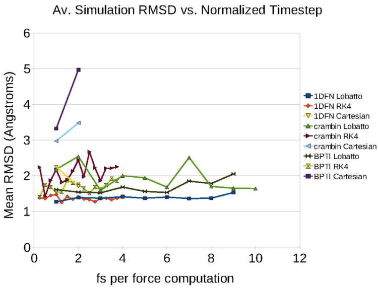
Average CRMSD in coordinates vs. timestep size over a 5ns simulation for various molecule-integrator combinations.

RMSF

Another test of simulation quality is to compare the fluctuation in various regions of the structure to that found experimentally in the crystal structures of the proteins. We have calculated a quantity called root mean square fluctuation (RMSF) for each residue in the simulation. The RMSF is calculated by taking the deviation of each residue’s position from its average position during the simulation. We compare this to the RMSF that would be expected from the crystal structure using the relation $B=\frac{8{\pi }^2}{3}{\mathit{RMSF}}^2$, where B is the crystallographic B-factor for each residue.

Figure 8 shows the difference between the simulation RMSF and the RMSF derived from the crystal structure’s B-factor for each residue, time step size, and for both the RK4 and Lobatto integrators. Each horizontal slice of these plots represents a single simulation, showing the protein sequence from N- to C-terminus with color indicating the difference between the simulated and experimentally-derived RMSF. Horizontal slices that are consistently close to 0 represent integrator-timestep combinations that replicate the experimentally expected dynamics. We note again that there are few trends that correlate consistently with timestep size. This result implies that the choice of simulation timestep and integrator have little bearing on the results of GNEIMO simulations, supplied that the timestep does not lead to a crash. Since all simulations appear to have similar outcome, we see that Lobatto is the most efficient choice for performing accurate simulations.

Figure 8.

Simulation RMSF - B factor derived RMSF for various proteins, integrators, and timesteps. RMSFs are calculated from the entire trajectory of each 5ns simulation. A value of 0 indicates that the RMSF of the residue on the x-axis observed in a simulation using the timestep on the y-axis matches the RMSF derived from the crystallographic B-factor. All distances in Å.

CONCLUSIONS

There are several theoretical and computational issues unique to CICMD models that need to be addressed for their proper use as an MD technique. Some of these issues are addressed in this paper, including a rigorous method to initialize velocities in generalized coordinates, an efficient algorithm for nulling the center of mass velocity, and a proposed explanation and solution for the flying ice cube effect in CICMD methods. We have developed a rigorous theoretical and computational framework and implemented these features in the GNEIMO CICMD method. The GNEIMO method supports various force-fields (CHARMM and AMBER), thermostats (Nosé-Hoover, Berendsen, and temperature rescaling thermostats), and solvation (GB/SA and distance dependent dielectric). Long timescale torsional dynamics simulations of proteins employing large timesteps lead to the flying ice cube effect with the Nosé-Hoover thermostat unless CM kinetic energies are periodically nulled.

We have implemented and tested advanced integrators such as RK4, Lobatto and adaptive timestep CVODE³³. Simulations of three crystal structures were performed with various timestep sizes for 5ns using the Lobatto and RK4 integrators. Both integrators were found to be stable and replicated crystal flexibility for normalized (fs per force field computation) timesteps as large as 10fs for Lobatto and 4fs for RK4. Within this range, the measured stability metrics from both types of integrator appeared to be largely independent of timestep size used. We conclude that the first-order Lobatto integrator allows for the largest normalized timestep and is thus the more efficient integration method for GNEIMO simulations.

We have also developed a toolkit to apply various clustering strategies which provides the user with several levels of coarse graining for the dynamic model of the protein. We have implemented the automated clustering of secondary structure elements as they are formed during the folding of proteins. This dynamic clustering tool is an adaptive scheme for coarse graining. Using the dynamic clustering tool we have folded four different proteins starting from their extended structure to molten globule-like native structures within 4 to 5Å of the crystal. In the GNEIMO software, we have created a framework for CICMD simulations that can be used in applications such as protein structure refinement, the study of domain motions in proteins, and ab initio structure prediction.

Some of the advancements required for robust CICMD simulations have been developed and implemented in the GNEIMO code but have yet to be tested numerically. These are: 1) dynamics of multiple chains including explicit solvent molecules and 2) use of the Fixman correction potential^21,37 to eliminate the systematic bias that stems from the holonomic constraints placed on the models in the calculation of thermodynamic properties from CICMD simulations.^5,38 We have derived a computational framework for calculating the Fixman compensating potential using the SOA techniques.³⁹ The numerical testing of the effect of this correction potential and comparison of its performance to force fields that have been tailored for CICMD simulations^4,40 are planned for future work.

SUMMARY.

We present a number of theoretical and computational methodological improvements necessary for the development of robust constrained internal coordinate molecular dynamics simulation techniques. To validate these improvements, we run simulations of three protein structures using different integration techniques and time steps, and find that the results of these simulations agree with experimental data. We also evaluate a higher level application of these techniques, called “Dynamic Clustering”, for the purpose of ab-initio protein folding and find that it samples the molten globule state for all four proteins tested.

References

- 1.Mazur A, RA A. J Biomol Struct Dyn. 1989;6:815. doi: 10.1080/07391102.1989.10507739. [DOI] [PubMed] [Google Scholar]
- 2.Mazur AK, Dorofeev VE, Abagyan RA. J Comput Phys. 1991;92:261. [Google Scholar]
- 3.Jain A, Vaidehi N, Rodriguez G. J Comput Phys. 1993;106:258. [Google Scholar]
- 4.Chen J, Im W, Brooks CL., III J Comput Chem. 2005;26:1565. doi: 10.1002/jcc.20293. [DOI] [PubMed] [Google Scholar]
- 5.Gibson KD, Scheraga HA. J Comput Chem. 1990;11:468. [Google Scholar]
- 6.Vaidehi N, Jain A, Goddard W. J Phys Chem. 1996;100:10508. [Google Scholar]
- 7.Vaidehi N, Goddard WA. J Phys Chem A. 2000;104:2375. [Google Scholar]
- 8.Schwieters CD, Clore GM. J Mag Res. 2001;152:288. doi: 10.1006/jmre.2001.2413. [DOI] [PubMed] [Google Scholar]
- 9.Flores SC, Sherman MA, Bruns CM, Eastman P, Altman RB. IEEE/ACM Transactions on Computational Biology and Bioinformatics. 2011;8:1247. doi: 10.1109/TCBB.2010.104. [DOI] [PMC free article] [PubMed] [Google Scholar]
- 10.Ryckaert J, Ciccotti G, Berendsen HJC. J Comput Phys. 1977;23:327. [Google Scholar]
- 11.Andersen HC. J Comput Phys. 1983;52:24. [Google Scholar]
- 12.Tobias DJ, Brooks CL., III J Comput Phys. 1988;89:5115. [Google Scholar]
- 13.Jain A. Journal of Guidance, Control and Dynamics. 1991;14:531. [Google Scholar]
- 14.Rodriguez G, Kreutz-Delgado K, Jain A. The International Journal of Robotics Research. 1991;10:371. [Google Scholar]
- 15.Chun HM, Padilla CE, Chin DN, Watanabe M, Karlov VI, Alper HE, Soosaar K, Blair KB, Becker OM, Caves LSD, et al. J Comput Chem. 2000;21:159. [Google Scholar]
- 16.Balaraman G, Park I, Jain A, Vaidehi N. J Phys Chem B. 2011;115:7588. doi: 10.1021/jp200414z. [DOI] [PMC free article] [PubMed] [Google Scholar]
- 17.Park I, Gangupomu V, Wagner J, Jain A, Vaidehi N. J Phys Chem B. 2012;116:2365. doi: 10.1021/jp209657n. [DOI] [PMC free article] [PubMed] [Google Scholar]
- 18.Gangupomu V, Park I-H, Wagner J, Jain A, Vaidehi N. 2012 Under Review. [Google Scholar]
- 19.Jain A, Park I-H, Vaidehi N. J Chem Theory Comput. 2012;8:2581. doi: 10.1021/ct3002046. [DOI] [PMC free article] [PubMed] [Google Scholar]
- 20.Still WC, Tempczyk A, Hawley RC, Hendrickson T. J Am Chem Soc. 1990;112:6127. [Google Scholar]
- 21.Fixman M. Proc Nat Acad Sci USA. 1974;71:3050. doi: 10.1073/pnas.71.8.3050. [DOI] [PMC free article] [PubMed] [Google Scholar]
- 22.Sugita Y, Okamoto Y. Chem Phys Lett. 1999;314:141. [Google Scholar]
- 23.Metropolis N, Rosenbluth AW, Rosenbluth MN, Teller AH, Teller E. J Comput Phys. 1953;21:1087. [Google Scholar]
- 24.Plimpton S. J Comput Phys. 1995;117:1. [Google Scholar]
- 25.Friedrichs MS, Eastman P, Vaidyanathan V, Houston M, LeGrand S, Beberg AL, Ensign DL, Bruns CM, Pande VS. J Comput Chem. 2009;30:864. doi: 10.1002/jcc.21209. [DOI] [PMC free article] [PubMed] [Google Scholar]
- 26.Mathiowetz A, Jain A, Karasawa N, Goddard W. Proteins: Structure, Function, and Bioinformatics. 1994;20:227. doi: 10.1002/prot.340200304. [DOI] [PubMed] [Google Scholar]
- 27.Jain A. Robot and Multibody Dynamics: Analysis and Algorithms. 1. Springer; 2010. [Google Scholar]
- 28.Harvey S, Tan R, Cheatham T. J Comput Chem. 1998;19:726. [Google Scholar]
- 29.Poursina M, Bhalerao K, Flores S, Anderson K, Laederach A. Methods Enzymol. 2011:73–98. doi: 10.1016/B978-0-12-381270-4.00003-2. [DOI] [PMC free article] [PubMed] [Google Scholar]
- 30.Frishman D, Argos P. Proteins. 1995;23:566. doi: 10.1002/prot.340230412. [DOI] [PubMed] [Google Scholar]
- 31.Jain A, Rodriguez G, Guidance J. Control, and Dynamics. 1993;16:830. [Google Scholar]
- 32.Jones D. J Mol Bio. 1999;292:195. doi: 10.1006/jmbi.1999.3091. [DOI] [PubMed] [Google Scholar]
- 33.Cohen SD, Hindmarsh AC. Computers in Physics. 1996;10:138. [Google Scholar]
- 34.Ozkan SB, Wu GA, Chodera JD, Dill KA. Proc Nat Acad Sci USA. 2007;104:11987. doi: 10.1073/pnas.0703700104. [DOI] [PMC free article] [PubMed] [Google Scholar]
- 35.Martyna GJ, Klein ML, Tuckerman M. J Chem Phys. 1992;97:2635. [Google Scholar]
- 36.Bond S, Leimkuhler B, Laird B. J Comput Phys. May151:114. [Google Scholar]
- 37.Fixman M. J Comput Phys. 1978;69:1527. [Google Scholar]
- 38.Go N, Scheraga H. Macromolecules. 1976;9:535. [Google Scholar]
- 39.Jain A. J Comput Phys. 1997;136:289. [Google Scholar]
- 40.Katritch V, Totrov M, Abagyan R. J Comput Chem. 2003;24:254. doi: 10.1002/jcc.10091. [DOI] [PubMed] [Google Scholar]
Associated Data
This section collects any data citations, data availability statements, or supplementary materials included in this article.