Protein Depth Calculation and the Use for Improving Accuracy of Protein Fold Recognition

Abstract

Protein structure and function are largely specified by the distribution of different atoms and residues relative to the core and surface of the molecule. Relative depths of atoms therefore are key attributions that have been widely used in protein structure modeling and function annotation. However, accurate calculation of depth is time consuming. Here, we developed an algorithm which uses Euclidean distance transform (EDT) to convert the target protein structure into a 3D gray-scale image, where depths of atoms in the protein can be conveniently and precisely derived from the minimum distance of the pixels to the surface of the protein. We tested the proposed EDT-based method on a set of 261 non-redundant protein structures, which shows that the method is 2.6 times faster than the widely used method proposed by Chakravarty and Varadarajan. Depth values by EDT method are highly accurate with a Pearson's correlation coefficient ≈1 compared to the calculations from exhaustive search. To explore the usefulness of the method in protein structure prediction, we add the calculated residue depth to the scoring function of the state of the art, profile–profile alignment based fold-recognition program, which shows an additional 3% improvement in the TM-score of the alignments. The data demonstrate that the EDT-based depth calculation program can be used as an efficient tool to assist protein structure analysis and structure-based function annotation.

1. Introduction

Most proteins perform the biochemical functions through the contact interactions with other ligands and proteins, where the detailed shapes of the molecules are essential to determine the interactions and functions. Accordingly, solvent accessibility (SA) of the atoms and residues, along with the surface of the molecules, has often been used to help analyze the structure and function of the proteins. Given a target structure, SA value can be calculated exactly by Euclidean Distance Transform based Surface generation program (EDTSurf) (Xu and Zhang, 2009) or approximately by Dictionary of Secondary Structure of Proteins (DSSP) (Kabsch and Sander, 1983).

However, SA usually specifies the residues in a binary form. For the residues that are completely buried in the protein structure, it does not describe where the residues locate inside the molecule. Depth, which measures the distance of each atom/residue to the solvent accessible surface in a continuous form, greatly complements the missing information by SA, which is important to analyze the fold and function of the protein. In fact, depths of residues in a protein are highly related to their effects of mutations on protein stability and on protein–protein interactions (Chakravarty and Varadarajan, 1999). Residue depth has also been widely used to specify protein folds in protein structure prediction (Zhou and Zhou, 2005; Liu et al., 2007; Wu and Zhang, 2008) and assist structure-based protein function annotation (Roy et al., 2012).

Despite the importance, there are by far very few methods that can calculate the depth for protein structures efficiently at either an atom level or a residue level. Chakravarty and Varadarajan (1999) proposed calculating the residue depth by rotating the protein in a box where the closest water molecule is identified for each atom in the protein. The accuracy of the method is compromised since the calculated depth value depends on the positions and orientations of the water molecules. One can also calculate the depth by first generating the explicit solvent accessibility surface (e.g., by EDTSurf or Michel Sanner's Molecular Surface (MSMS) (Sanner et al., 1996)) and then identifying the vertex on the triangulated surface which is the closest one to the atom (Yuan and Wang, 2008; Zhang et al., 2008). However, the computation of this kind of method is quite time-consuming since all the atoms in the protein need to be searched against the huge number of vertices on the mesh surface.

In a recent study, we have established the unified relationship between the three kinds of macromolecular surfaces and Euclidean distance transform (EDT) theoretically and developed a fast algorithm for generating their triangulated surfaces precisely (Xu and Zhang, 2009). In this work, we apply the EDT technique to the calculation of protein atom depth and residue depth. The algorithm is fast since the explicit triangulated surface is not required. To investigate the efficiency and accuracy of this method, we compare the computational time and depth value with that by Chakravarty and Varadarajan (CV). We also analyze the relation of protein depth with the commonly used radius of gyration and solvent accessibility and prove that they are independent structural features. Matching of residue depth is also added to the scoring function of our fold recognition program, which shows incremental improvement over solvent accessibility.

2. Material and Methods

2.1. Depth definition

Atom depth is the shortest distance between the center of the atom and the outer solvent accessible surface (SAS) of the molecule, as illustrated in Figure 1. SAS is the area traced out by the center of a probe sphere when it is rolling over the whole molecule (Lee and Richards, 1971). When an atom is exposed (e.g., atom i in the figure), its depth will equal to the sum of its van de Waals radius and the radius of the probe sphere r_p which is often set to 1.4 Å. For atoms that are completely buried inside (e.g., atoms j and k in the figure), their solvent accessibilities are all equal to zero, but their depths may be different. Residue depth is the average value of the atom depths of all the atoms in the residue.

FIG. 1.

Illustration of three atoms with different depth values in a 2D plane. The outer boundary stands for the solvent accessible surface.

The definition of atom depth by Chakravarty and Varadarajan is a little different, which is the shortest distance to the explicit bulk water rather than the solvent accessible surface. Since water molecules do not have spherical shapes and may have different poses around the molecule, this difference will result in the slightly different depth values.

2.2. Euclidean distance transform

Euclidean distance transform (EDT) is the transformation that converts a digital binary image to another gray-scale image where the value of each pixel is the minimum Euclidean distance between that pixel and the boundary. We have developed a fast algorithm that can conduct EDT in arbitrary dimensional space (Xu and Li, 2006). EDT has been widely used in the fields of image processing and computer graphics, in applications of skeleton extraction (Choi et al., 2003), shortest path planning (Shih and Wu, 2004), and geometric shape description (Xu and Li, 2007).

Given a protein structure, we suppose it has N atoms, each of which locates at p_i and has a van der Waals radius r_i. To calculate the atom depth in the protein, we first build the solvent accessible solid using Equation (1), which is the union of all the spheres with radius equal to the sum of the van der Waals radius and the radius of the probe sphere. The union operation is conducted in the discrete 3D space using space-filling technique, with each sphere represented by a set of grid points.

(1)

Then we can easily determine the outer shell of the solvent accessible solid, which is the discrete representation of solvent accessible surface . EDT is then carried out to the shell, which converts the whole solid into Euclidean distance map (EDM). We can directly obtain the shortest Euclidean distance of each atom to the shell, which happens to be the depth value of the atom, as formulized in Equation (2). Although there are several other distance functions, such as City-block distance and Chessboard distance, only Euclidean distance has the direct relationship with the three macromolecular surfaces as well as the depth.

(2)

In the original CV method and its recent extension (Tan et al., 2011), non-bulk water molecules are removed in the regions of narrow cavities and internal voids. Otherwise, atoms around those regions will have small values of depths. Using Equation (1), the solvent accessible solid has already filled most of the empty space in the same regions since the radius of each atom is enlarged by the radius of the probe sphere. Therefore, EDT method is not affected in those special regions and has the consistent depth values with that by the CV method.

Figure 2 shows an example of the EDT result to the same shape of the SAS in Figure 1, where the red curve stands for the SAS. After the EDT, every position has a shortest distance to the SAS, as represented by the gray-scale pixel value in the image. The lighter the point is, the longer distance to the surface it will have. Based on the definition of the depth, we can see that the gray-scale pixel value calculated by the EDT at each point exactly is the depth value of that point. In the figure, the centers of the three atoms, as represented by the blue dots, have different depth values.

FIG. 2.

Illustration of EDT to the solvent accessible surface (red) in a 2D plane. Centers of the three atoms are marked in blue.

Solvent accessibility of each residue is defined as the ratio of the total SAS area of all the atoms in the residue to the maximum SAS area of that residue type. Hence, we have to build the explicit triangulated surface from the discrete shell by surface triangulation algorithms such as the Marching Cube method (Lorensen and Cline, 1987). Different than the solvent accessibility derivation, depth calculation does not require the generation of the explicit triangulated SAS.

Given the shell of the discrete SAS, we can also calculate the depth of each atom by exhaustive search (ES). That is to say, we search for the point on the shell that is the closest to the center of the atom.

2.3. Protein fold recognition using residue depth

For template-based structure prediction, the most crucial step is template identification and fold recognition, which determines the initial structural fold for the query sequence. Solvent accessibility has been proved to be a useful term for fold recognition, in threading programs such as SP⁴ (Liu et al., 2007) and MUlti-Sources ThreadER (MUSTER) (Wu and Zhang, 2008). The matching score is often defined as the difference between the predicted solvent accessibility of the query sequence and the accurately pre-calculated solvent accessibility of each template structure. They did not directly use the residue depth for matching. Instead, a structure profile is built using fragments of similar RMSDs (Root-mean-square deviation) and depth values.

Here, residue depths of the query sequence are predicted by a two-layer back-propagation neural network (Rumelhart et al., 1986), which has architecture similar to that used for the solvent accessibility prediction (Xu and Zhang, 2012). The scoring function for matching depth of residue i in the query sequence and residue j in the template is the negative logarithm of the probability of residue type aa(i) having depth difference Δ_RD(i, j) divided by the background probability, which is close to that of SPARKSX (Yang et al., 2011). Similar equations are used for the matching of secondary structure types and solvent accessibility.

(3)

The complete scoring function for matching two residues is given in Equation (4), where the profile matching term (Xu and Zhang, 2013) is the dot-product of the frequency profile calculated from multiple sequence alignments and the log-odds profile from the Position-Specific Substitution Matrix, both of which come from Position-Specific Iterative Basic Local Alignment Search Tool (PSI-BLAST) (Altschul et al., 1997). The weighting factors w₁, w₂, and w₃ in the equation are equal to 1.3, 1.0, and 0.2, separately. Needleman–Wunsch (Needleman and Wunsch, 1970) dynamic programming algorithm is adopted to generate the optimal global alignments between every two proteins.

(4)

3. Results and Discussion

3.1. Visualization of depth

In order to visually check the depth information generated by the method described above, we have embedded the EDT-based depth calculation algorithm into our Macromolecular Visualization and Processing (MVP) program.

Figure 3 shows two snapshots of the MVP visualization result of a hypothetical protein from thermus thermophilus HB8 (PDB ID: 1whz, chain A), which contains 122 residues and 937 atoms. Atoms in the left figure are in ball-stick style. Red color means high value of atom depth, while blue means low. In the right image, we show the protein structure in backbone style, where the color of each residue is also correlated with its residue depth. From both images, we can clearly see the layers of the protein structure, especially the hydrophobic core which is in red.

FIG. 3.

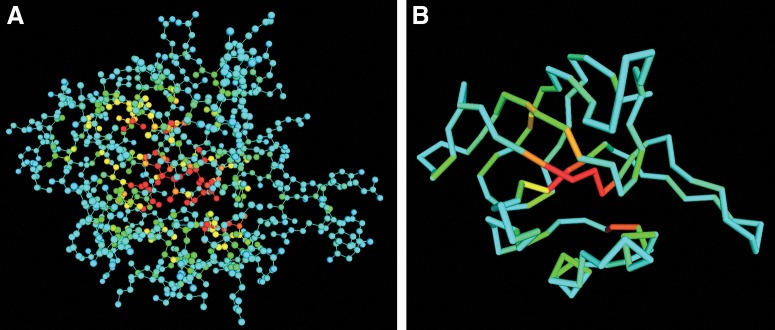
Visualization of (A) atom depth and (B) residue depth of protein 1whz chain A by MVP.

3.2. Depth distributions of different residue types

Since different residue types have different hydrophobicities, their depth distributions should also be different. Therefore, we choose 36,556 protein domains used by our threading programs (Wu and Zhang, 2007, 2008) for validation, which can be downloaded at http://zhanglab.ccmb.med.umich.edu/library/. Those structures are nonhomologous to each other with sequence identity cutoff 70%. Protein chains which contain multiple domains are discarded from the list in this test, since multiple-domain proteins are often not well packed.

The distributions of residue depths of the 20 residue types are shown in Figure 4, which are arranged in the order of their hydrophobicity scales (Kyte and Doolittle, 1982). Residue depths normally are in the range of 2.9 Å and 8.9 Å. Almost all the residue depths are less than 5 Å for the 8 hydrophilic residues on the top TWO rows. Tryptophan (TRP) and serine (SER) have similar hydrophobicities, but TRP has more depths that are deeper than 5 Å. This is probably because TRP has a longer side-chain and its depth can be large even part of the residue is exposed. For the six most hydrophobic residues on the bottom two rows, more depth values are around 6 Å than that of the hydrophilic residues. However, majority of the depths are still close to 3.1 Å, which means many hydrophobic residues still locate around the surface of the domain structures. It is understandable if the protein is stable only in the complex form instead of the monomeric form. Hydrophobic residues in the interface will have deep residue depths if we treat the complex as a whole.

FIG. 4.

Distributions of residue depths for the 20 residue types.

3.3. Comparison of depth generation methods

We compare the depth results by the algorithm described by Chakravarty and Varadarajan (CV) and exhaustive search (ES) and EDT-based method (EDT) mentioned above. The test set here we choose contains 261 nonhomologous protein chains randomly selected from the PISCES list (Wang and Dunbrack, 2003). In the CV algorithm, 216 three-site water molecules are put in a box with edge length 18.856 Å. We rotate each protein at 25 different orientations in the box and find the shortest distance to the outer water molecule for each atom. For both ES and EDT, we first enlarge each protein four times and put it into its minimum bounding box. Then we create the voxel shell that represents the solvent accessible surface. ES method directly searches the closest voxel for each atom without using EDT. The EDT method only requires the EDT to the voxel shell to get the depth value for each atom.

We first compare the similarities of the depth values generated by the three methods. The Pearson's correlation coefficients (PCC) of the residue depths by the three kinds of methods are shown in Table 1. Results by ES and EDT methods are highly close to each other. Although CV method is quite different to the other two, it still has a high correlation (>0.90) with them.

Table 1.

Comparison of Residue Depths by Methods of Chakravarty and Varadarajan (CV), exhaustive search (ES), and EDT-Based Method (EDT)

	CV	ES	EDT
PCC
CV	1.00	0.91	0.90
ES	0.91	1.00	1.00
EDT	0.90	1.00	1.00
Time(sec)	2.23	1.69	0.88

The difference of the depth values by CV and EDT mainly comes from two sources. First, the depth definitions by the two methods are slightly different, which have been described before. Second, since CV is an approximation method, depth value is highly dependent on the water molecules placed outside of the protein. Sometimes the depth value is close to the real depth if the water molecule happens to be the closest one, while sometimes it does not. In contrast, depth values calculated by ES and EDT are close to the real one. The only error of the EDT method stems from the discretization of the protein which makes the discrete shell not exactly the same as the actual continuous SAS.

We then compare the average computational time by the three methods, which is tabulated in the last row of the Table 1. The calculation is performed on a single node with a 2.27 GHZ Intel E5520 Xeon processor and 24 GB memory. EDT method is 2.6 times faster than CV and 1.9 times faster than ES. We can imagine the CPU time taken by the ES method will increase rapidly if we increase the scale factor to generate the more accurate SAS shell. We have also tried the new version of the DEPTH program using the CV method in (Tan et al., 2011), which takes even longer time (data not shown) due to the extensive search for the nonbulk water molecules.

Compared with the accuracy, speed may be not an issue if we only calculate the depth once for each protein structure. However, a lot of computational resources could be saved if depth information of thousands of structures has to be calculated. For example, in the application of protein fold recognition, the non-redundant template library often contains more than 40,000 protein chains/domains extracted from the Protein Data Bank (PDB) (Berman et al., 2000).

3.4. Depth versus radius of gyration

Radius of gyration (RG) refers to the root mean square distance of the protein atoms from the center of gravity. Due to the simplicity of calculation, RG has been widely used to characterize the global shape and compactness of protein tertiary structure in protein structure prediction (Zhang et al., 2003) and function annotation (Roy and Zhang, 2012). However, due to the high specificity of protein tertiary structure packing, the simple RG calculation cannot precisely reflect the shape and residue distribution related to the exposed surfaces on specific proteins. In this section, we examine the quantitative relation of RG and depth calculated from EDT technique which highlights the advantage of depth in characterizing the overall shape of protein tertiary structure.

We compare the radius of gyration with the maximum residue depth (MD) and the average residue depth (AD) in Figure 5(A) and 5(B) separately. The data are acquired still based on the 36,556 domain structures in our threading template library. In the left figure, we can see that the two features have some correlation in most of the regions. Most times, when the radius of gyration is large, the maximum depth will also be very high. Especially when the protein structure is compact and has a globular shape, its maximum depth will be highly correlated with its radius of gyration, such as the protein in Figure 6(A). It is the chain A of the Desulfovibrio vulgaris apoflavodoxin-riboflavin complex (PDB ID: 1bu5), which has the radius of gyration around 14 Å. Since the five beta-strands and four helices are densely organized, the maximum depth is also very high and very close to the radius of gyration.

FIG. 5.

Comparison of radius of gyration with (A) the maximum residue depth and (B) the average residue depth. Reduced numbers of points are shown in the figure by Origin.

FIG. 6.

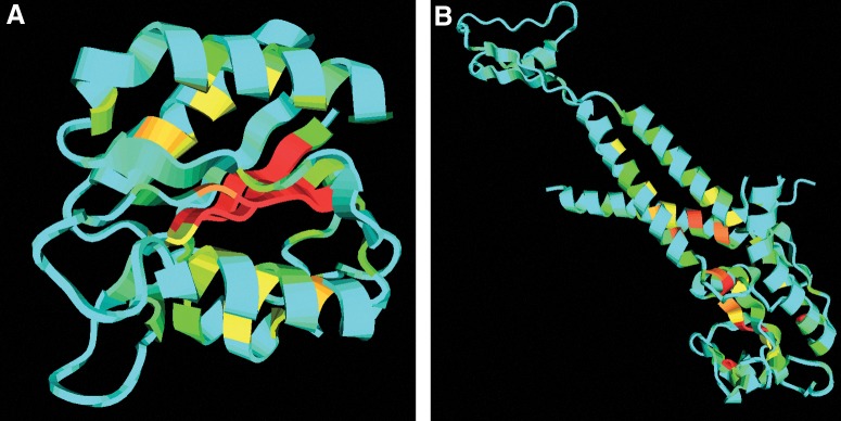
Cartoon style of two protein chains with color representing the residue depth. (A) 1bu5 chain A, radius of gyration = 13.840 Å, maximum depth = 10.459 Å; (B) 1ijg chain L, radius of gyration = 30.428 Å, maximum depth = 7.603 Å.

There are also exceptions where the radius of gyration is high but the maximum depth is extremely low. This is because some single-domain proteins (e.g., a super-long helix) have loose arrangements of secondary structure elements which make depth values of most residues very low. Figure 6(B) shows the chain L of the Bacteriophage phi29 head-tail connector protein (PDB ID: 1ijg). If we solely consider this chain, only one end is well-shaped. There are three other helices in the middle, which connect two short beta-strands and one short helix in the other end. This structure has an extremely large radius of gyration of 30 Å. However, since this chain is not compact and most of the residues are exposed, the maximum depth is only 7.603 Å.

The scatter plot between the average depth and the radius of gyration in Figure 5(B) has the similar distribution to that between the maximum depth and the radius of gyration in Figure 5(A). This is because the Pearson's correlation coefficient between the maximum depth and the average depth is very high (0.92 in Table 2).

Table 2.

Pearson's Correlation Coefficients Between the Four Global Features

	RG	RS	MD	AD
RG	1.00	0.96	0.07	0.02
RS	0.96	1.00	0.05	−0.02
MD	0.07	0.05	1.00	0.92
AD	0.02	−0.02	0.92	1.00

Another measurement describing the overall shape is the radius of the bounding sphere (RS), which is the minimum radius of the sphere that could cover all the atoms in the protein structure. It has a very high correlation (0.96) with the radius of gyration, which is probably because the center of the bounding sphere is close to the center of gravity for most proteins.

All the PCC values between the four global structural features are listed in Table 2. As we have explained, RG and RS have no obvious correlations with the maximum and average depths due to the irregular shapes of some proteins. For RG and RS, distances are calculated between the positions of all the residues and one fixed point (e.g., the center of gravity or the center of the bounding sphere). Those distances have no strong physical meaning when the protein has a nonglobular shape and residues are far away from this point. On the contrary, depth is a local measurement since different atoms have different closest points on the SAS.

From the above analysis, we can draw the conclusion that RG and RS are very rough measurements of protein shapes. The maximum/average residue depth provides independent information to RG/RS. They can help characterize the unique features of protein tertiary structures including the overall 3D shape and in particular the residue distribution relative to the surface exposition.

3.5. Depth versus solvent accessibility

The range of solvent accessibility value is in [0, 1] after we normalize the SAS area by the maximum SAS area of each residue type. For the residues which are partially exposed to solvation, they may have the same solvent accessibility but different depth values due to the various sizes of the different residue types. By comparing the non-zero solvent accessibility and residue depth for each residue type based on the 36,556 protein domains, we find that SA and RD follow an exponential function:

(5)

In Table 3, we list values of the three parameters in equation (5) for all the 20 amino acids. As expected, those parameters are different for different residue types. The amplitude parameter A seems proportional to the size of each amino acid. For example, small amino acids glycine (GLY) and alanine (AlA) have small amplitudes, while large amino acids arginine (ARG) and TRP have big amplitudes. More hydrophilic residues tend to have a larger scale parameter t, such as ARG and lysine (LYS), while more hydrophobic residues have a higher y parameter [e.g., phenylalanine (PHE) and isoleucine (ILE)].

Table 3.

Parameters of the Exponential Functions for the 20 Amino Acid Types

	y	A	t		y	A	t
ARG	2.96	1.20	0.14	SER	2.89	0.84	0.11
LYS	2.96	1.18	0.16	THR	2.97	0.90	0.12
ASN	2.93	0.98	0.11	GLY	2.87	0.64	0.06
ASP	2.91	0.97	0.11	ALA	2.96	0.77	0.07
GLU	2.92	1.09	0.12	MET	3.08	1.17	0.08
GLN	2.95	1.09	0.12	CYS	2.93	0.98	0.11
HIS	3.00	1.20	0.11	PHE	3.17	1.29	0.07
PRO	3.04	0.83	0.11	LEU	3.16	1.05	0.06
TYR	3.08	1.35	0.10	VAL	3.13	0.95	0.07
TRP	3.12	1.44	0.10	ILE	3.18	1.05	0.06

In Figure 7, we compare solvent accessibility and residue depth for aspartic acid as an example. Generally, points in the scatter plot follow the exponential function, as illustrated by the black fitting curve. Depth difference is not significant when solvent accessibility is high, which means majority part of the residue is exposed. However, when SA is low (majority is buried), depth value can be quite different. Diversity of depth values might be caused by two reasons. The first one is the different relative positions and orientations of the residue to the solvent accessible surface while the second one is the different side-chain conformations. The shape of each residue type is not unique due to the degrees of freedom of side-chain torsion angles.

FIG. 7.

Scatter plot between solvent accessibility and residue depth for aspartic acid. Black curve is the fitting curve by an exponential function. Reduced numbers of points are shown in the figure by Origin.

3.6. Comparison of fold recognition results

We first group the 20 amino acids into two sets, hydrophobic residues and hydrophilic residues based on their hydrophobicity scales (Kyte and Doolittle, 1982) and then evaluate their prediction errors for both solvent accessibility and residue depth. From Table 4, we clearly see that hydrophobic residues have smaller prediction error for solvent accessibility than hydrophilic residues because their solvent accessibility values are close to zero at most times. For residue depth, difference between the two types of residues is even larger. Hydrophobic residues have almost twice as much error as hydrophilic residues because their various depth values are harder to predict. This table highly suggests that the two structural features should be used together to avoid the high prediction error of one residue type.

Table 4.

Difference Between the Real Value and Predicted Value of Solvent Accessiblity and Residue Depth for the Two Different Residue Types

	Solvent accessibility	Residue depth
Hydrophobic residues	0.075	0.118
Hydrophilic residues	0.101	0.060
Ratio	0.743 = 1/1.347	1.967

We select 148 “hard” sequences as the test set, whose difficulties are defined by LOMETS (Wu and Zhang, 2007) meta-threading server after homologous templates are removed from the template library for each sequence. Alignment accuracy of the initial backbone structure, which is directly copied from the corresponding template, is measured by the Template Modeling Score (TM-score) (Zhang and Skolnick, 2004). We start with the sequence profile matching term in the scoring function and add structural features one by one. The detailed result is shown in Table 5. The three kinds of structural features indeed have positive effects on fold recognition, which provide complementary information to sequence profile matching. As expected, adding residue depth also could help improve alignment accuracy and optimize template selection without increasing the alignment length, which is about 3% higher than that only uses secondary structure types and solvent accessibility.

Table 5.

Threading Alignment Accuracy of Hard Sequences as Evaluated by TM Score

	1st	Coverage	Best in top20	Coverage
Profile	0.309	0.893	0.399	0.902
Profile+SS	0.353	0.885	0.440	0.881
Profile+SS+SA	0.369	0.880	0.454	0.894
Profile+SS+SA+RD	0.379	0.877	0.455	0.881
MUSTER	0.344	0.875	0.439	0.888

The evaluation of alignments produced by MUSTER is shown in the last row of the table. Although MUSTER also includes the depth information, the direct depth matching in this paper seems more efficient, which is about 10% better than MUSTER.

In addition, we have also tried to include ϕ and ψ torsion angles and 4-Cα-based torsion angle into the scoring function, as did by MUSTER. However, they could not further improve the alignment accuracy, probably because the prediction errors are high for those features (>20° on average), although they seem to be independent structural features.

4. Conclusions

We have developed a computational algorithm for the fast and accurate calculation of the atom/residue depth through Euclidean distance transform. The method was tested on a set of 261 nonredundant protein structures. It was shown that EDT-based method is 2.6 times faster than the widely used method developed by Chakravarty and Varadarajan, but the accuracy of the EDT-based method is higher than that of the latter compared with the actual depth from exhaustive search.

Depth data are systematically analyzed in the large-scale proteins that cover the entire PDB library at the sequence identity cutoff of 70%. It is found that the maximum/average residue depth has no obvious correlation with the commonly used radius of gyration and radius of the bounding sphere. Hence, the maximum/average depth could be considered as a new geometric feature for describing the global shape of protein tertiary structure. It is of potential use for protein fold classification and structure comparison.

When the residue is not completely buried inside of the protein molecule, solvent accessibility and residue depth follow an exponential relation. Different residue types have different parameters of the fitting functions and different distributions of residue depths even their hydrophobic scales are close to each other. The various sizes of the amino acids seem to be the major factors which cause the differences.

When the residue is completely buried inside of the protein structure, residue depth becomes a useful measurement as solvent accessibility of the residue remains zero in this situation. Hence, we use residue depth as a complementary feature to the solvent accessibility as an additional term in the scoring function for fold recognition, which indeed could improve template selection and alignment accuracy. On the other hand, depth attribution clearly illustrates the shape distribution of residues in the protein structure and could help to identify the cavity region, which potentially contains the active site or binding site. Correctly identification of residues around this region could accelerate the structure-based binding site prediction and aid the consequent function annotation (Roy and Zhang, 2012).

The source code and executable program for computing atom depth and residue depth are freely available at http://zhanglab.ccmb.med.umich.edu/EDTSurf/. The associated software MVP (Macromolecular Visualization and Processing) for visualizing the depth information is downloadable at http://zhanglab.ccmb.med.umich.edu/MVP/.

Acknowledgments

The project is supported in part by the NSF Career Award (DBI 1027394), and the National Institute of General Medical Sciences (GM083107, GM084222).

Disclosure Statement

The authors declare that no competing financial interests exist.

References

- 1.Altschul SF. Madden TL. Schaffer AA, et al. Gapped BLAST and PSI-BLAST: A new generation of protein database search programs. Nucleic Acids Res. 1997;25:3389–3402. doi: 10.1093/nar/25.17.3389. [DOI] [PMC free article] [PubMed] [Google Scholar]
- 2.Berman HM. Westbrook J. Feng Z, et al. The Protein Data Bank. Nucleic Acids Res. 2000;28:235–242. doi: 10.1093/nar/28.1.235. [DOI] [PMC free article] [PubMed] [Google Scholar]
- 3.Chakravarty S. Varadarajan R. Residue depth: A novel parameter for the analysis of protein structure and stability. Structure. 1999;7:723–732. doi: 10.1016/s0969-2126(99)80097-5. [DOI] [PubMed] [Google Scholar]
- 4.Choi WP. Lam KM. Siu WC. Extraction of the Euclidean skeleton based on a connectivity criterion. Pattern Recog. 2003;36:721–729. [Google Scholar]
- 5.Kabsch W. Sander C. Dictionary of protein secondary structure: Pattern recognition of hydrogen-bonded and geometrical features. Biopolymers. 1983;22:2577–2637. doi: 10.1002/bip.360221211. [DOI] [PubMed] [Google Scholar]
- 6.Kyte J. Doolittle RF. A simple method for displaying the hydropathic character of a protein. J Mol Biol. 1982;157:105–132. doi: 10.1016/0022-2836(82)90515-0. [DOI] [PubMed] [Google Scholar]
- 7.Lee B. Richards FM. The interpretation of protein structures: Estimation of static accessibility. J Mol Biol. 1971;55:379–400. doi: 10.1016/0022-2836(71)90324-x. [DOI] [PubMed] [Google Scholar]
- 8.Liu S. Zhang C. Liang S. Zhou Y. Fold recognition by concurrent use of solvent accessibility and residue depth. Proteins. 2007;68:636–645. doi: 10.1002/prot.21459. [DOI] [PubMed] [Google Scholar]
- 9.Lorensen WE. Cline HE. Marching cubes: A high resolution 3d surface construction algorithm. Comput Graph. 1987;21:163–169. [Google Scholar]
- 10.Needleman SB. Wunsch CD. A general method applicable to the search for similarities in the amino acid sequence of two proteins. J Mol Biol. 1970;48:443–453. doi: 10.1016/0022-2836(70)90057-4. [DOI] [PubMed] [Google Scholar]
- 11.Roy A. Yang J. Zhang Y. COFACTOR: An accurate comparative algorithm for structure-based protein function annotation. Nucleic Acids Res. 2012;40:W471–477. doi: 10.1093/nar/gks372. [DOI] [PMC free article] [PubMed] [Google Scholar]
- 12.Roy A. Zhang Y. Recognizing protein-ligand binding sites by global structural alignment and local geometry refinement. Structure. 2012;20:987–997. doi: 10.1016/j.str.2012.03.009. [DOI] [PMC free article] [PubMed] [Google Scholar]
- 13.Rumelhart DE. Hinton GE. Williams RJ. Learning representations by back-propagating errors. Nature. 1986;323:533–536. [Google Scholar]
- 14.Sanner MF. Olson AJ. Spehner JC. Reduced surface: An efficient way to compute molecular surfaces. Biopolymers. 1996;38:305–320. doi: 10.1002/(SICI)1097-0282(199603)38:3%3C305::AID-BIP4%3E3.0.CO;2-Y. [DOI] [PubMed] [Google Scholar]
- 15.Shih FY. Wu YT. Three-dimensional Euclidean distance transformation and its application to shortest path planning. Pattern Recog. 2004;37:79–92. [Google Scholar]
- 16.Tan KP. Varadarajan R. Madhusudhan MS. DEPTH: A web server to compute depth and predict small-molecule binding cavities in proteins. Nucleic Acids Res. 2011;39:W242–248. doi: 10.1093/nar/gkr356. [DOI] [PMC free article] [PubMed] [Google Scholar]
- 17.Wang G. Dunbrack RL., Jr. PISCES: A protein sequence culling server. Bioinformatics. 2003;19:1589–1591. doi: 10.1093/bioinformatics/btg224. [DOI] [PubMed] [Google Scholar]
- 18.Wu S. Zhang Y. LOMETS: A local meta-threading-server for protein structure prediction. Nucleic Acids Res. 2007;35:3375–3382. doi: 10.1093/nar/gkm251. [DOI] [PMC free article] [PubMed] [Google Scholar]
- 19.Wu S. Zhang Y. MUSTER: Improving protein sequence profile-profile alignments by using multiple sources of structure information. Proteins. 2008;72:547–556. doi: 10.1002/prot.21945. [DOI] [PMC free article] [PubMed] [Google Scholar]
- 20.Xu D. Li H. Euclidean distance transform of digital images in arbitrary dimensions. LNCS. 2006;4261:72–79. [Google Scholar]
- 21.Xu D. Li H. Shape analysis of volume models by Euclidean distance transform and moment invariants. 10th IEEE International Conference on Computer-Aided Design and Computer Graphics. 2007:437–440. [Google Scholar]
- 22.Xu D. Zhang Y. Generating triangulated macromolecular surfaces by Euclidean distance transform. PLoS One. 2009;4:e8140. doi: 10.1371/journal.pone.0008140. [DOI] [PMC free article] [PubMed] [Google Scholar]
- 23.Xu D. Zhang Y. Ab initio protein structure assembly using continuous structure fragments and optimized knowledge-based force field. Proteins. 2012;80:1715–1735. doi: 10.1002/prot.24065. [DOI] [PMC free article] [PubMed] [Google Scholar]
- 24.Xu D. Zhang Y. Toward optimal fragment generations for ab initio protein structure assembly. Proteins. 2013;81:229–239. doi: 10.1002/prot.24179. [DOI] [PMC free article] [PubMed] [Google Scholar]
- 25.Yang Y. Faraggi E. Zhao H. Zhou Y. Improving protein fold recognition and template-based modeling by employing probabilistic-based matching between predicted one-dimensional structural properties of query and corresponding native properties of templates. Bioinformatics. 2011;27:2076–2082. doi: 10.1093/bioinformatics/btr350. [DOI] [PMC free article] [PubMed] [Google Scholar]
- 26.Yuan Z. Wang ZX. Quantifying the relationship of protein burying depth and sequence. Proteins. 2008;70:509–516. doi: 10.1002/prot.21545. [DOI] [PubMed] [Google Scholar]
- 27.Zhang H. Zhang T. Chen K. Shen S. Ruan J. Kurgan L. Sequence based residue depth prediction using evolutionary information and predicted secondary structure. BMC Bioinform. 2008;9:388. doi: 10.1186/1471-2105-9-388. [DOI] [PMC free article] [PubMed] [Google Scholar]
- 28.Zhang Y. Kolinski A. Skolnick J. TOUCHSTONE II: A new approach to ab initio protein structure prediction. Biophys J. 2003;85:1145–1164. doi: 10.1016/S0006-3495(03)74551-2. [DOI] [PMC free article] [PubMed] [Google Scholar]
- 29.Zhang Y. Skolnick J. Scoring function for automated assessment of protein structure template quality. Proteins. 2004;57:702–710. doi: 10.1002/prot.20264. [DOI] [PubMed] [Google Scholar]
- 30.Zhou H. Zhou Y. Fold recognition by combining sequence profiles derived from evolution and from depth-dependent structural alignment of fragments. Proteins. 2005;58:321–328. doi: 10.1002/prot.20308. [DOI] [PMC free article] [PubMed] [Google Scholar]