Hierarchical structural mapping for globally optimized estimation of functional networks

Abstract

In this study, we propose a framework to map functional MRI (fMRI) activation signals using diffusion tensor imaging (DTI)-tractography. This framework, which we termed functional by structural hierarchical (FSH)mapping, takes into account the origin of fMRI brain activation to construct the “N-step reachable structural maps” - a series of vectors that denote signal propagation after the N-th step tracing of the structural connectivity matrix from the origin. Linear combinations of these N-step reachable maps are then used to predict the observed fMRI signals. Additionally, a utilization matrix, which numerically estimates whether the inclusion of a specific structural connection better predicts fMRI, can be constructed and estimated using simulated annealing. We tested the proposed framework on a visual fMRI task in a sample of body dysmorphic disorder (BDD) subjects and comparable healthy controls. Group differences were inferred by comparing the observed utilization differences against 10,000 permutations under the null hypothesis. Results revealed that BDD subjects under-utilized several key local connections in the visual system, which may help explain previously reported fMRI findings and further elucidate the underlying pathophysiology of BDD.

1 Introduction

How the brain is organized into functional networks remains an elusive question. Despite widespread use of functional neuroimaging, inferences on network properties have largely been based on associative activation patterns; its limited temporal resolution hinders an understanding of dynamic interactions between spatially defined nodes. Advanced modeling techniques such as Dynamic Causal Modeling [1] provide estimates of complex neuronal dynamic interactions estimated from BOLD signal patterns, but may be practical for understanding only a small number of nodes.

Inferences about network dynamical interactions on a larger scale could potentially be derived using strategies involving structural to functional mapping. This is based on the assumption that a system's structural connectivity pattern provides a framework for determining information available as inputs from certain regions and its outputs and potential influence on other regions [2]. Such an approach could utilize a combination of DTI-tractography to estimate brain white matter connectivity and functional magnetic resonance imaging (fMRI) to estimate the neuronal activity coupled to blood flow changes in anatomical regions that comprise nodes of the network.

Several structural to functional mapping approaches have been proposed [2-9]. Some have focused on specific, limited regional activation patterns [2, 3] while others have developed models for understanding functional connections in larger set of regions comprising networks or systems [4-9]. However, to our knowledge no study has used structural to functional mapping to estimate information transfer on a systems-wide level. We therefore developed a model to parsimoniously explain overall observed activation patterns with the assumption that the system is comprised of a set of interacting nodes.

To test this approach, we applied it to understanding activation patterns within the visual system. The visual system has been well characterized in monkeys and humans and can be reliably activated with functional neuroimaging paradigms. In addition, previous studies have provided models for a temporal sequence of activation, particularly for the “first wave” of information transfer (see, for example [10, 11]), from V1 to V2 and other visual cortical areas, followed by temporal and parietal regions. This allows us to make several simplifying assumptions about direction of information transfer. We tested our model in a dataset consisting of healthy human controls and individuals with body dysmorphic disorder (BDD). Individuals with BDD have perceptual distortions in which they misperceived defects in their appearances [12]. Previous fMRI studies in BDD found abnormal visual processing in primary and secondary visual processing systems for face and inanimate object (house) stimuli [13-15]. To better characterize these findings, we thus developed a strategy for functional by structural hierarchical mapping to estimate step-wise activation patterns in the visual system. Here, the word “hierarchical” refers to the n-step structural maps used for model fitting. The fMRI portion of this dataset, which utilized well-characterized house visual stimuli, was previously analyzed for group differences using the general linear model [13]. Here we demonstrate a model of hierarchical structural to functional mapping that, under several simplifying assumptions, elaborates on previous results by providing estimates of structural connection utilization within the visual system.

2 Methods

2.1 Data collection

Eleven unmedicated participants with BDD and 13 healthy controls, aged 20 to 48 years, were scanned in a 3-T Siemens Allegra MRI scanner. Diffusion-weighted MR imaging (DWI) data were acquired using single-shot spin-echo echo-planar imaging (EPI) (field of view=240mm; voxel size=2.5×2.5×3.0mm, with 0.75 mm gap; TR/TE=7400/96ms; flip angle 9°). We collected 44 contiguous axial slices aligned to the AC-PC line along 34 gradient-sensitizing directions with b=1000s/mm² and one minimally diffusion-weighted scan. DWI data were corrected for eddy current artifacts using FSL toolbox (http://www.fmrib.ox.ac.uk/fsl/fdt/fdt_eddy.html). fMRI data came from a previous object-processing fMRI study; subject selection, acquisition and preprocessing are as previously described [13]. fMRI stimuli consisted of photographs of houses that contained only low spatial frequency (LSF) information [16], in order to more sensitively probe configural and holistic visual processing.

2.2 Brain network computation

We computed whole-brain deterministic DTI tractography using Diffusion Toolkit with the Fiber Assignment by Continuous Tracking (FACT) algorithm [17] and a maximum turn angle of 35 degrees. Cortical regions of interest (ROIs) were defined using the Harvard Oxford Cortical probabilistic atlas. The masks were set to a liberal threshold of 10% to allow for the inclusion of tissue along the gray-white matter interface, where DTI tractography estimates are most reliable [18]. To register these ROIs to each subject's DTI space, we used FSL's FLIRT program [19] to determine the optimal affine transformation between the MNI152 T1 average brain (in which the Harvard Oxford probabilistic atlases are based) and each subject's unique FA image, using a mutual information-based cost function. We applied the resulting transformation to register the 26 visual pathway related ROIs to each subject's DTI space. For each pair of ROIs, the number of fibers connecting them was counted to construct a structural connectivity matrix (a fiber was considered to connect two ROIs if it originated in the first ROI and terminated in the second, or vice versa). Thus, this matrix was symmetric, with the diagonal entries set to zero (no self connections).

To generate functional MRI signals for each region of interest, we computed the percentage signal change using the Featquery tool in FSL to estimate BOLD signal differences between the house stimuli and baseline.

2.3 Functional by structural hierarchical (FSH)mapping

Several assumptions and simplifications are needed in order to perform FSH mapping, outlined step-by-step as follows:

1. A collection of cortical anatomical regions or “nodes” is determined to be activated during the fMRI task, and cortical fMRI activation is assumed to originate in a specific region(s) (the “origin”), in this case the left and right intracalcarine cortices.

2. N-step reachable structural maps, defined as regions reachable from the origin at the n-th step of structural connections, are computed by tracing the anatomical connectivity (according to the structural connectivity matrix C) from the origin.

3. Nodes that are reached in the first n steps will be excluded from later steps. All connections between nodes are hypothesized to be excitatory. Moreover, feedback or interactions between nodes that have been reached is assumed to be numerically negligible.

4. The presence of an edge connecting any node pair in the structural connectivity matrix predicts the existence of neuroanatomical connections between regions, which may are may not be “utilized” in the particular fMRI task of interest. A connection between node i and j is considered “utilized” if including the anatomical connection between node i and node j better predicts the overall fMRI activation. This is modeled by a binary utilization matrix U (i.e., if U(i,j)=1, then the structural connection between nodes i and j are utilized in the fMRI task; zero otherwise)

5. The observed fMRI activation pattern is assumed to be explained by linear combinations of n-step reachable structural maps.

Now, we illustrate how to set up the FSH mapping using the BDD house processing example. In step 1, a total of 26 visual system ROIs were carefully selected from the group mean fMRI activation maps overlaid on the Harvard-Oxford cortical probabilistic atlas for house stimuli viewing vs. baseline, for combined BDD and healthy control groups. These 26 regions are the (bilateral) lateral occipital cortex superior division (nodes 1,2), lateral occipital cortex inferior division (3,4), intracalcarine cortex (5,6), precuneus cortex (7,8), cuneal cortex (9,10), parahippocampal gyrus posterior division (11,12), lingual gyrus (13,14), temporal fusiform cortex anterior division (15,16), temporal fusiform cortex posterior division (17,18), temporal occipital fusiform cortex (19,20), occipital fusiform cortex (21,22), supracalcarine cortex (23,24), and occipital pole (25,26).

As the fMRI task was a visual task, we thus assumed that cortical fMRI signals originated in the bilateral primary visual cortex (V1 or intracalcarine cortex; nodes 5 and 6). Mathematically, this is represented by a 26-element “activation” column vector A, whose entries are all zeros except for bilateral V1 (where A takes values of 1). In steps 2-4, we first observe that 0-step reachable map is A itself, and define the 1-step reachable map as (U ◦ C) (here the circle operator denotes the entry-wise or Hadamard product of two matrices of the same dimension). The n-step reachable structural maps (A_n) were then determined by the iterative application of the following procedure:

A₀ = A, C_o = C; for n = 0, 1, …,

1. initialize C_n+1 = C_n;

2. compute the column vector A_n+1 = (U ◦ C_n)· A_n; for all i such that A_n+1(i) > 0, set all entries in the i – th column and i – th row of C_{n +1} to zero.

Lastly, we fit the following linear equation so that the entire set of observed fMRI activations in the visual system, S, can be explained by linear combinations of A_n

$$S=w_0{A}_0+w_1{A}_1+w_2{A}_2+\dots w_n{A}_n+e$$

Here, S is the fMRI signal column vector (26×1) and e is the error term. The optimization of the FSH mapping is achieved in two parts. First, U was initialized as a 26×26 matrix whose every entry took a value of 1 (i.e., all structural connections were utilized). We then fixed U and the linear equation above was fitted to determine the weights (w₀, w₁, w₂, etc in the above equation) and to calculate the fitting errors. For the second part of the optimization, the weights were fixed, and data from all subjects in each group were pooled together to estimate a group-level optimal U using the simulated annealing algorithm (thus yielding two U matrices, one for the BDD and one for the control group). To this end, we perturbed U (from state i to state j) by randomly picking one element in U and changing its value (between 0 and 1). The acceptance criterion determined whether the new state j was accepted from the current state i by applying the following decision rule with respect to an artificial cooling temperature (c).

$$P_c\{\mathit{\text{accept}}j\}=\{\begin{array}{cc}1& \mathit{\text{if}}e\left(j\right)\le e\left(i\right)\\ exp\left(\frac{e\left(i\right)-e\left(j\right)}{c}\right)& \mathit{\text{if}}e\left(j\right)>e\left(i\right)\end{array}$$

Where e(i) and e(j) are the linear fitting residuals. This perturbation was repeated numerous times until the solution space was adequately sampled and the global minimum reached.

2.4 Determining statistical significance for observed utilization group differences

As structural connection strengths vary across edges, utilization differences for connections that have on average higher fiber counts should be considered potentially more significant. As a result, we devised a statistic dU, by summing up all rows and columns of the difference matrix (subtracting the U of the control group from that of the BDD) weighted by the mean connectivity matrix C̄ (structural connectivity matrices averaged across all study participants).

$$dU=\sum _{i,j=1}^{26}\left[\right(U^{\mathit{\text{BDD}}}-U^{\mathit{\text{control}}}\left)\mathrm{o}\overline{C}\right]$$

Here, dU measures the overall group utilization differences, and permutation testing can be conducted to determine whether the observed dU reaches statistical significance. To this end, we performed 10,000 permutations by randomly re-assigning each subject's diagnosis (into two groups of size 11 and 13). At each permutation, the test statistic dU was re-computed and recorded, and the observed dU was then ranked against the re-sampled dUs. If the observed dU was relatively extreme and ranked among the top 5%, then we determined that the observed utilization group difference has reached statistical significance at a p value of 0.05.

3 Results

Linear fitting errors vs. the level of n-step structural maps used for model fitting for one subject is shown in Figure 1. Figure 2 summarizes fitting results for all subjects in both groups. Linear combinations of 1-, 2-, and 3-step structural maps were tested. Three-level structural maps provided sufficient linear fitting, which was further improved with simulated annealing.

Fig. 1.

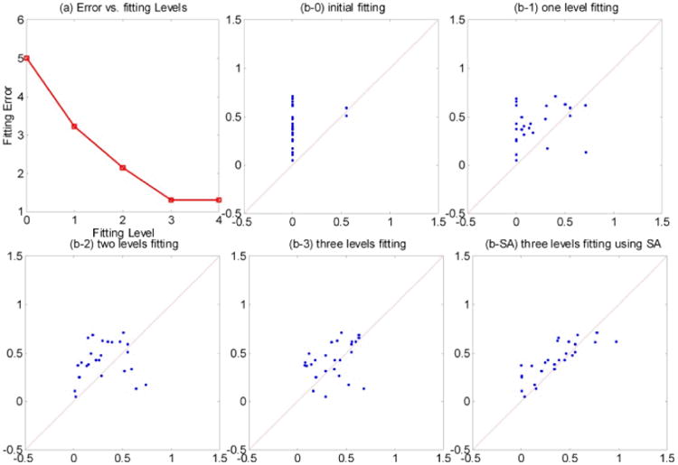
(a) Fitting errors vs. fitting levels in one study participant. (b-0 through b-3) Functional by structural hierarchical (FSH) mapping results in the same subject using 0, 1, 2, and 3-level structural maps. The y axis indicates observed fMRI % signal change and the x axis the predicted fMRI % signal change (data points that are perfectly predicted by the proposed method would lie along the x=y line). (b-SA) The 3-level linear fitting in addition to the simulated annealing (SA) step. Visually, the SA step further improves data fitting.

Fig. 2.

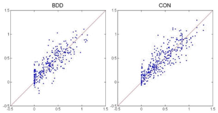
Group fitting. This shows the fitting of data points, pooled from all subjects in each group, using the proposed 3-level fitting with simulated annealing. The y axis indicates observed fMRI % signal change and the x axis the predicted fMRI % signal change. (Note that predicted values were set to be greater than zero as one of the simplifying assumptions of the model).

Group differences in the binary utilization matrices (BDD-control) weighted by the mean connectivity strength (note that this matrix is symmetrical, and thus its (i, j) and (j,i) elements indicate the utilization difference for the same structural connection) are shown in Figure 3. According to this model, the control group utilized several more structural connections than the BDD group (the most significant differences, marked A to C in Figure 3, are structural connections between the left intracalcarine cortex and left lingual gyrus, the right intracalcarine cortex and right lingual gyrus, and the right temporal occipital fusiform cortex and right temporal fusiform cortex, posterior division. These connections are visualized in Figure 4. Permutation tests confirmed that the observed utilization group difference reached statistical significance (p = 0.0329).

Fig. 3.

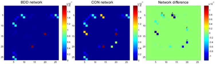
Utilization matrices (left panel for BDD and middle panel for controls) and their differences (BDD-control; right panel) weighted by the mean edge strength (values in color bar). In the right panel, the most significant utilization differences (entries in blue; not utilized in BDD) represent connections between the following regions: left intracalcarine cortex and left lingual gyrus (A), right intracalcarine cortex and right lingual gyrus (B), right temporal occipital fusiform cortex and right temporal fusiform cortex, posterior division (C), left intracalcarine cortex and right precuneus cortex (D), right intracalcarine cortex and left cuneal cortex (E), and right parahippocampal gyrus, posterior division and right temporal occipital fusiform cortex (F).

Fig. 4.

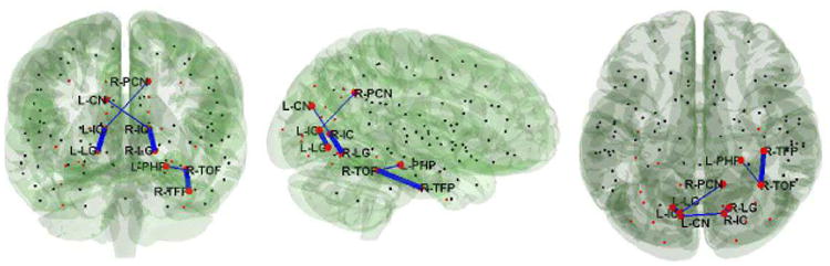
Additional anatomical connections (marked in blue) utilized in the control relative to the BDD group. Here, the centers of the 26 visual system ROIs are represented by red dots. (The centers of other nodes not used in this study are shown for reference and are represented as black dots). The thicker lines correspond to connections A to C, and thinner lines D to F in the right panel of Figure 3. L/R indicates left/right, and IC, LG, TOF, TFP, PCN, CN, PHP denotes the intracalcarine cortex, the lingual gyrus, the temporal occipital fusiform cortex, the temporal fusiform cortex posterior division, the precuneus, the cuneal cortex, and the parahippocampal gyrus respectively.

4 Discussions and Conclusions

These results are consistent with previous fMRI results for house processing, which found relative hypoactivity in the BDD group vs. controls in the lingual gyrus, precuneus, and parahippocampal gyrus [13]. Moreover, the use of FSH mapping provides additional information about utilization of structural connections that may explain observed fMRI differences; an inference from this is that individuals with BDD may have abnormally low information transfer between both primary and secondary visual cortical regions, and within higher-order temporal lobe visual processing systems. Results must be considered in light of multiple simplifying assumptions made to aid in this initial model development, and in light of small sample size. Future models that account for feedback, inhibitory interactions, and deactivation are necessary for more accurate estimations. Nevertheless, FSH may serve as a useful tool for integrating structural connectivity with fMRI data for improved understanding of functional activation patterns.

References

- 1.Friston KJ, Harrison L, Penny W. Dynamic causal modelling. Neuroimage. 2003;19(4):1273–302. doi: 10.1016/s1053-8119(03)00202-7. [DOI] [PubMed] [Google Scholar]
- 2.Saygin ZM, et al. Anatomical connectivity patterns predict face selectivity in the fusiform gyrus. Nat Neurosci. 2011;15(2):321–7. doi: 10.1038/nn.3001. [DOI] [PMC free article] [PubMed] [Google Scholar]
- 3.Johansen-Berg H, et al. Changes in connectivity profiles define functionally distinct regions in human medial frontal cortex. Proceedings of the National Academy of Sciences of the United States of America; 2004; pp. 13335–13340. [DOI] [PMC free article] [PubMed] [Google Scholar]
- 4.Passingham RE, Stephan KE, Kotter R. The anatomical basis of functional localization in the cortex. Nat Rev Neurosci. 2002;3(8):606–16. doi: 10.1038/nrn893. [DOI] [PubMed] [Google Scholar]
- 5.Chulwoo L, et al. Brain state change detection via fiber-centered functional connectivity analysis. Biomedical Imaging: From Nano to Macro; 2011 IEEE International Symposium on; 2011. [Google Scholar]
- 6.Skudlarski P, et al. Brain Connectivity Is Not Only Lower but Different in Schizophrenia: A Combined Anatomical and Functional Approach. Biological Psychiatry. 2010;68(1):61–69. doi: 10.1016/j.biopsych.2010.03.035. [DOI] [PMC free article] [PubMed] [Google Scholar]
- 7.Deligianni F, et al. Inference of functional connectivity from structural brain connectivity. Biomedical Imaging: From Nano to Macro; 2010 IEEE International Symposium on; 2010. [Google Scholar]
- 8.Honey CJ, et al. Predicting human resting-state functional connectivity from structural connectivity. Proceedings of the National Academy of Sciences; 2009; pp. 2035–2040. [DOI] [PMC free article] [PubMed] [Google Scholar]
- 9.Varkuti B, et al. Quantifying the Link between Anatomical Connectivity, Gray Matter Volume and Regional Cerebral Blood Flow: An Integrative MRI Study. PLoS One. 2011;6(4) doi: 10.1371/journal.pone.0014801. [DOI] [PMC free article] [PubMed] [Google Scholar]
- 10.Felleman DJ, Van Essen DC. Distributed Hierarchical Processing in the Primate Cerebral Cortex. Cerebral Cortex. 1991;1(1):1–47. doi: 10.1093/cercor/1.1.1-a. [DOI] [PubMed] [Google Scholar]
- 11.Lamme VA, Roelfsema PR. The distinct modes of vision offered by feedforward and recurrent processing. Trends Neurosci. 2000;23(11):571–9. doi: 10.1016/s0166-2236(00)01657-x. [DOI] [PubMed] [Google Scholar]
- 12.American Psychiatric Association. Diagnostic and statistical manual of mental disorders : DSM-IV-TR. 4th. Washington, DC: American Psychiatric Association; 2000. p. xxxvii.p. 943. [Google Scholar]
- 13.Feusner JD, et al. Abnormalities of visual processing and frontostriatal systems in body dysmorphic disorder. Archives of General Psychiatry. 2010;67(2):197–205. doi: 10.1001/archgenpsychiatry.2009.190. [DOI] [PMC free article] [PubMed] [Google Scholar]
- 14.Feusner JD, et al. Visual information processing of faces in body dysmorphic disorder. Archives of General Psychiatry. 2007;64(12):1417–25. doi: 10.1001/archpsyc.64.12.1417. [DOI] [PubMed] [Google Scholar]
- 15.Feusner JD, et al. Abnormalities of object visual processing in body dysmorphic disorder. Psychological Medicine. 2011:1–13. doi: 10.1017/S0033291711000572. [DOI] [PMC free article] [PubMed] [Google Scholar]
- 16.Iidaka T, et al. Spatial frequency of visual image modulates neural responses in the temporo-occipital lobe. An investigation with event-related fMRI. Cognitive Brain Research. 2004;18:196–204. doi: 10.1016/j.cogbrainres.2003.10.005. [DOI] [PubMed] [Google Scholar]
- 17.Mori S, van Zijl PC. Fiber tracking: principles and strategies - a technical review. NMR Biomed. 2002;15(7-8):468–80. doi: 10.1002/nbm.781. [DOI] [PubMed] [Google Scholar]
- 18.Morgan VL, et al. Integrating functional and diffusion magnetic resonance imaging for analysis of structure-function relationship in the human language network. PLoS One. 2009;4(8):e6660. doi: 10.1371/journal.pone.0006660. [DOI] [PMC free article] [PubMed] [Google Scholar]
- 19.Jenkinson M, et al. Improved optimization for the robust and accurate linear registration and motion correction of brain images. Neuroimage. 2002;17(2):825–41. doi: 10.1016/s1053-8119(02)91132-8. [DOI] [PubMed] [Google Scholar]
- 20.Venkataraman A, et al. Joint Modeling of Anatomical and Functional Connectivity for Population Studies. IEEE Transactions on Medical Imaging. 2012;31(2):164–182. doi: 10.1109/TMI.2011.2166083. [DOI] [PMC free article] [PubMed] [Google Scholar]
- 21.Koch MA, et al. An investigation of functional and anatomical connectivity using magnetic resonance imaging. Neuroimage. 2002;16:241–250. doi: 10.1006/nimg.2001.1052. [DOI] [PubMed] [Google Scholar]
- 22.Sporns O, et al. Theoretical neuroanatomy: Relating anatomical and functional connectivity in graphs and cortical connection matrices. Cerebral Cortex. 2000;10:127–141. doi: 10.1093/cercor/10.2.127. [DOI] [PubMed] [Google Scholar]
- 23.Honey CJ, et al. Network structure of cerebral cortex shapes functional connectivity on multiple time scales. Proc Nat Acad Sci. 2007;104:10240–10245. doi: 10.1073/pnas.0701519104. [DOI] [PMC free article] [PubMed] [Google Scholar]