

Abstract
When some of the regressors can act on both the response and other explanatory variables, the already challenging problem of selecting variables when the number of covariates exceeds the sample size becomes more difficult. A motivating example is a metabolic study in mice that has diet groups and gut microbial percentages that may affect changes in multiple phenotypes related to body weight regulation. The data have more variables than observations and diet is known to act directly on the phenotypes as well as on some or potentially all of the microbial percentages. Interest lies in determining which gut microflora influence the phenotypes while accounting for the direct relationship between diet and the other variables A new methodology for variable selection in this context is presented that links the concept of q-values from multiple hypothesis testing to the recently developed weighted Lasso.
Keywords: False discovery rate, Microbial data, q-Values, Variable selection, Weighted Lasso
1. Introduction
Variable selection is an omnipresent issue in biological studies where data typically involve more predictor variables than samples. Variable selection in this context is challenging and has been studied extensively in recent years. Various methods include the Lasso (Tibshirani, 1996) and its extensions (Yuan and Lin, 2006; Zou, 2006; Meinshausen and Bühlmann, 2010), least angle regression (LARS) (Efron and others, 2004), and selection via controlling false discovery rates (FDRs) (Benjamini and Hochberg, 1995; Storey, 2003). A problem, not yet directly addressed by these methods, is selecting regressors when some act on both the response and other explanatory variables. To handle this new challenge, we develop a novel method that extracts weights from q-values in multiple hypothesis testing (Storey, 2003), and uses them in the weighted Lasso (Zou, 2006).
Structured variable selection is needed when there are multiple types of variables and some knowledge is available about the hierarchy between the variables. For example, in a dietary treatment study of mice, biologists aim to understand how diet and different gut microflora affect phenotypes related to body weight regulation. The challenge is selecting those microbes that affect weight, while incorporating the fact that diet is known to regulate body weight (Bray and others, 2012) and may affect some microbial groups (Abnous and others, 2009; Li and others, 2009). Thus, the objective is to select variables that affect the response after accounting for diet.
Another example stems from screening tests for early detection of a disease. To detect psychosis among low-income Latinos (Wang and others, 2011), a screening questionnaire was used. Questions were divided into root and stem questions such that stem questions were asked only if the patient answered specific root questions. A key interest is identifying which questions yield an accurate detection of psychosis, while maintaining the hierarchy between root and stem questions. Ignoring the hierarchy may yield a model with only stem questions, which is uninterpretable.
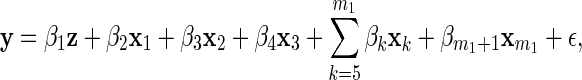
Our proposed methods for structured variable selection handle these and other examples well. Let the sample size be n and y=(y1,…,yn)T be the response variable. Let m0 denote the number of fixed covariates (e.g. the number of diets or root questions in the examples above), and we denote these variables by n×1 vectors zj, j=1,…,m0. Let m1 denote the number of other covariates (e.g. number of gut microflora or stem questions), and we denote these n×1 variables as xk, k=1,…,m1. Without loss of generality, we assume that all variables are standardized to have mean zero and sample variance 1, so that the intercept is excluded from the regression model. We also assume that m0+1≤n (see Section 2.3.1 for an explanation), but that m0+m1=m≥n.
Thus, our goal is to find the variables among (x1,…,xm1) that affect the response after accounting for (z1,…,zm0). To our knowledge, such a problem has never been considered. It differs from that in Yuan and others (2009) where variables are clustered and obey a heredity principle: each cluster contains a dominant variable, and variables in a cluster are considered for selection only if the dominant one is selected. In our case, variables are not clustered, and there is scientific evidence to require that fixed variables (z1,…,zm0) be included in the model. For example, when modeling body weight regulation, diet should be included; or in developing screening tests for psychosis, root questions that reveal symptoms preceding a first psychotic episode (Phillips and others, 2000) should be included. Given the problem's novelty, there is no obvious benchmark to which we can compare proposed methods. Instead, we develop a method which links q-values from multiple hypothesis testing with a weighted Lasso, and compare its results with those based on thresholding Benjamini and Hochberg (1995) adjusted p-values.
The paper is organized as follows. Section 2 describes two methods for structured variable selection. The first uses Benjamini–Hochberg (BH)-adjusted p-values and the second uses a weighted Lasso with q-values from multiple hypothesis testing. We demonstrate the advantages of the second method over the first through a simulation study in Section 3 and in supplementary material available at Biostatistics online. We also show that using partial correlation coefficients instead of q-values in the weighted Lasso has similar advantages. In Section 4, we describe the microbial data which motivated this methodology and analyze the data. Section 5 concludes the paper.
2. Multiple testing and variable selection
2.1. Lasso and weighted Lasso
The Lasso (Tibshirani, 1996) is a widely used method for variable selection, and has had several extensions since its initial presentation. A particular variant is the weighted Lasso, which has the adaptive Lasso (Zou, 2006) as a special case. In the context of linear regression, the weighted Lasso generalizes the Lasso by incorporating data-dependent weights. Recalling that m0+m1=m, and defining β=(β1,…,βm)T and X=(z1,…,zm0,x1,…,xm1), the adaptive Lasso minimizes
 |
(2.1) |
Here, λ is a regularization parameter and  , j=1,…,m, denotes the ordinary least squares estimate after regressing y on X. In practice, of course, we actually minimize (2.1) by using the standard Lasso procedure. First, we transform the covariates in (2.1), i.e.
 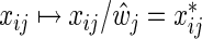 ,
, 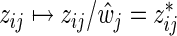 , and define
  and
and  . Then we solve for
  by minimizing
  and obtain the final estimates
 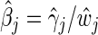 .
.
Although the adaptive Lasso uses weights  , any appropriate data-dependent weights can be used. Charbonnier and others (2010) and Bergersen and others (2011) showed that weights which incorporate prior knowledge or relevant external information on the covariates yields more stable results. We build upon these ideas, but introduce a new type of weight function based on q-values in such a way that structured variable selection is incorporated.
2.2. Use of q-values
The notion of q-values is a by-product of controlling FDRs (Benjamini and Hochberg, 1995), which is a means for quantifying statistical significance in multiple hypothesis testing. In multiple hypothesis testing, one simultaneously tests multiple null hypotheses, among which some are true nulls and the remaining are false. The FDR is the expected proportion of falsely rejected hypotheses. Popular FDR controlling methods involve transforming the p-values from the multiple hypotheses tested, and then thresholding them at a level α. Two such p-value adjustments are the Benjamini and Hochberg (1995) procedure, and q-values (Storey, 2003) which are defined explicitly in Section 2.3.2. In general, null hypotheses with small adjusted p-values are rejected but not those with large adjusted p-values. If the cut-off is α and the null hypotheses are independent or satisfy certain dependency structures, then among the rejected null hypotheses, α×100% of them are expected to be false positives, leading to an FDR of α.
We identify significant explanatory variables with two methods using these adjusted p-values. The first thresholds BH-adjusted p-values, and the second uses q-values in the weighted Lasso.
2.3. Thresholding adjusted p-values
2.3.1. p-values accounting for known effective predictors
One approach to determining the significance of variables xk, k=1,…,m1, is to test m1 appropriate null hypotheses, or even multiple families of hypothesis tests, while accounting for the variables (z1,…,zm0) that are known to affect the response. We do this by testing each of (x1,…,xm1) separately given (z1,…,zm0), i.e. for k=1,…,m1, we run a linear regression of y on (z1,…,zm0,xk), and compute the p-value pk for the effect of xk in this regression. Assuming m0+1≤n, these regressions are valid.
2.3.2. BH-adjusted p-values
When testing these m1 null hypotheses, adjusting p-values using the BH procedure is useful for quantifying statistical significance and maintaining low FDRs. Using the ordered p-values p(1)≤⋯≤p(m1), the BH-adjusted p-values are  and
and  for k=m1−1,m1−2,…,1. Variables included in the model (i.e. significant variables) are those with BH-adjusted p-values ≤α for some pre-specified α. With this threshold, it is expected that α×100% of the deemed significant variables are actually not significant when the test statistics are independent (Benjamini and Hochberg, 1995) or positively dependent (Benjamini and Yekutieli, 2001). To minimize the false discoveries, we choose α small but not too small, say 0.15.
Although thresholding BH-adjusted p-values is popular, a major drawback is that it individually, rather than collectively, investigates the significance of each xk given (z1,…,zm0), k=1,…,m1. Such a process suppresses to some extent the intercorrelations between the x's as shown in the simulation study (Section 3). Thus, to overcome this issue, we propose a modified weighted Lasso with q-values as weights (Section 2.4).
2.3.3. Definition of q-values
Like BH-adjusted p-values, q-values are a monotone transformation of the p-values from multiple hypothesis testing. Their explicit form involves the empirical process FDR(t), which is the associated FDR based on rejecting null hypotheses with p-values ≤t for t∈[0,1]. That is,  , where S(t)=#{pk:pk≤t,k true null} is the number of false positives, and R(t)=#{pk:pk≤t} is the total number of null hypotheses rejected. Storey and Tibshirani (2003) proposed estimating FDR(t) with
  , where the estimate of the true proportion of null hypotheses is
 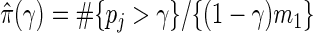 for a tuning parameter γ. The optimal γ which leads to the best estimate
  may be computed using the bootstrap or a smoothing spline (Storey and Tibshirani, 2003). In our applications, we use the latter. From
  , q-values are estimated as
  , and as
  for k=m1−1,m1−2,…,1. When
  , the q-values are the BH-adjusted p-values.
2.4. Modified weighted Lasso
Variable selection via thresholding adjusted p-values is a well-known technique, but our approach is based upon a novel use of q-values as weights in the weighted Lasso. In general, estimates from the weighted Lasso are those that minimize (2.1); however, we are going to replace the weights  by appropriately chosen non-negative weights wj.
The selection of weights is important as it can influence the stability and accuracy of the parameter estimates. Bergersen and others (2011) showed that more stable results are achieved if the weighting scheme uses external information. They proposed weights wj(y,X,V)=1/|gj(y,X,V)|κ for j=1,…,m, κ>0, where X=(z1,…,zm0,x1,…,xm1), V is a matrix of external information, and gj are appropriately chosen functions. They showed two explicit examples for gj: one based on Spearman correlation coefficients, and the second based on ridge regression coefficients.
Our proposed method for structured variable selection builds upon these ideas, although it is distinctly different in implementation. Recall that zj, j=1,…,m0, are not subject to selection, and xk, k=1,…,m1, are subject to selection. To emphasize this distinction, we set weights wj=1/g1(y,X) on zj and wm0+k=1/g2(y,X) on xk, where g1 and g2 are chosen to direct the variable selection process. Specifically, if g1 and g2 are chosen so that  can be made arbitrarily close to zero, then the z's are selected before the x's. In practice, we recommend choosing g1 so that small enough weights are placed on the z's to ensure their inclusion in the model before the x's enter.
The choice for g2 should emphasize that highly influential x's are included before the less important ones, as well as include information about the relationship between the x's, z's, and y's. One such measure is the q-values (Section 2.3.2) in that statistically significant x's tend to have small q-values, whereas non-significant x's have large q-values. Other measures providing similar information are the test statistics’ magnitudes, p-values (Section 2.3.1), BH-adjusted p-values (Section 2.3.2), and the partial correlation between the x's and y's after controlling for the z's: all of which are essentially monotone transformations of each other. Through various simulation studies, we find that weights based on any of these quantities have similar results. A key feature of these quantities is that they account for (z1,…,zm0) having an effect on the response. Weights that ignore this aspect result in important variables being ignored; see supplementary material available at Biostatistics online.
We now describe how q-values lead to meaningful weights for the weighted Lasso, though weights based on any of the above monotone transformations are also useful. Letting g2 be any non-increasing function, one may define q-value-dependent weights by  ; a simple choice is g2(q)=1/qκ, κ>0. These q-value-dependent weights have several advantages in the selection process among x1,…,xm1. First, we can penalize variables which seem non-significant (i.e. have large q-values) more than those which are highly influential (i.e. have small q-values). Second, the weighted Lasso allows us to simultaneously assess the impact of multiple variables (z1,…,zm0,x1,…,xm1) on the response y, and thus better handles any correlation between the explanatory variables. As shown in Section 3, when an insignificant variable is strongly correlated with another explanatory variable, the weighted Lasso correctly disregards this insignificant variable more often than does thresholding BH-adjusted p-values. Finally, certain choices of g2 can make the weighted Lasso give FDRs ≤α for well-chosen λ in (2.1), or δ in (2.2).
For different choices of g1 and g2, we will use the standard Lasso to perform variable selection. In particular, we use the LARS algorithm (Efron and others, 2004), which provides the entire sequence of model fits in the Lasso path, along with estimated parameter coefficients. The best descriptive model will be that which minimizes the penalized loss function
 |
(2.2) |
where δ>0, p denotes the number of predictors in the selected model, SSEp denotes the residual sum of squares for the model, and  is an appropriate estimator of the model error variance. For example, when n>m,
  can be the residual mean square when using all available variables, and when n<m,
  can be the variance of the response vector y (Hirose and others, 2011). This loss function balances the residual sum of squares of a fitted model with the number of non-zero parameter estimates, and when δ=2, the loss function is Mallows’ Cp. Instead of (2.2), other model selection criteria may be used; see Müller and Welsh (2010).
An important detail of (2.2) is the choice of δ as different δ values yield different model fits and observed FDRs. We propose selecting the optimal δ based on K-fold cross-validation. Fix δ=δ0 and randomly partition the data into K non-overlapping equal-sized subsets. Then, do the following: (i) remove data subset k; (ii) apply the LARS algorithm to the remaining K−1 data subsets, and select the model that minimizes Mn(δ0,p); (iii) extract the estimate  from the minimizing model and compute
 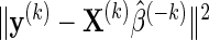 , where y(k) and X(k), respectively, denote the response and explanatory variables for the data subset k that was removed. Lastly, (iv) repeat the above three steps for each k=1,…,K and compute the cross-validation score
  . The optimal δ is
  where, as in our simulation study, δ0=0.75,…,2. Results were similar across K=4,…,10; thus, we suggest using K=10.
In our experience, the cross-validation requires two modifications. First, δ0 that minimizes CV (δ0) is not necessarily unique; thus, take δopt as the average of the minimizers. Second, δopt is a random variable that depends on the random partitioning of the data. Repeated applications of K-fold cross-validation may yield different δopt and thus different variables selected, especially when the signals are sparse and small. Martinez and others (2011) also noted this and suggested performing the K-fold cross-validation repeatedly, say 100 times, to develop a complete understanding of the variables selected. The idea, thus, is to repeat the K-fold cross-validation multiple times, and retain those variables that were selected at least 80% of the time, say. This procedure works well in practice (see Section 3), and has the added benefit of remedying the Lasso's limitation: when n<m, the Lasso can select at most n variables because it involves solutions to a convex optimization problem (Zou and Hastie, 2005). Because different variables may be selected in each run of the K-fold cross-validation and variables that appear at least 80% of the time are retained, there is the possibility that more than n variables are in the final model. Stability selection (Meinshausen and Bühlmann, 2010) is another way to select more than n variables.
3. Simulation study
We evaluated the performance of the proposed methods on simulated data that are similar to our empirical example in Section 4. We supposed there were two diet groups with 20 subjects in each, and generated m1+1 explanatory variables as follows. First, we generated a binary diet indicator z where, for each subject i=1,…,40, zi=I(i>20)−I(i≤20). Then we generated xk=(x1,k,…,x40,k)T, k=1,…,m1, such that xik=uik+zivk, where uik were independent uniform (0,1) random variables, v1,…,v0.75m1 were independent uniform (0.25, 0.75) random variables, and v0.75m1+1,…,vm1 were identically zero. Thus, we created m1 variables, x1,…,xm1 where the first 75% of the x's depend on z. Finally, we generated the response vector as
 |
(3.1) |
where ϵ is normally distributed with mean 0 and covariance σ2I. We set m1=40, σ2=0.5, and β=(4.5,3,−3,−3,0T,3)T where 0T is an (m1−4)-dimensional vector of zeros. In summary, x1,…,xm1 were generated according to four distinct categories:
Group 1. x1,x2,x3 depend on diet and act on y even after taking into account diet;
Group 2. x4,…,x0.75m1 depend on diet and do not act on y;
Group 3. x0.75m1+1,…,xm1−1 neither depend on diet, nor act on y;
Group 4. xm1 does not depend on diet, but acts on y.
We generated 1000 independent data sets, and applied three variable selection procedures. We computed BH-adjusted p-values, and q-values associated with the significance of xk, k=1,…,m1, after accounting for diet z as in Section 2.3. Our first method thresholds BH-adjusted p-values over a range of α values in [0.01,0.20]. Our second method is a q-weighted Lasso with weights  on z and
  on xk. Our third method is a ρ-weighted Lasso with weights
  on z and
  on xk, where
  denotes the estimated partial correlation between xk and y after controlling for z. For both weighted Lasso methods, the best model was chosen using the loss function (2.2), where we evaluated the performance over a range of δ values in [0.25,2]. We also applied our data-driven way for choosing δopt and the variables selected: on each simulated data, we repeated the 10-fold cross-validation (Section 2.4) 100 times. This led to 100 possibly different δopt's and, thus, 100 possibly different ways variables were selected. Ultimately, we retained variables that were chosen at least 80% of the time in the 100 runs. It is important to note that we did not use the average of the 100 δopt's to select variables. Supplementary material available at Biostatistics online contains additional results, including those for m1=1000, different β vectors, α thresholds, weight functions, and δ values. Some of the choices show lower true-positive rates or unacceptable false-positive rates.
For all methods, variables within each group behaved similarly; thus, we report the average percentages of time variables in each group were selected and the observed FDRs. Among all methods, the reliable one will routinely select variables in Groups 1 and 4, rarely or never select variables in Groups 2 and 3, and thus, have low FDRs.
Thresholding BH-adjusted p-values at level α yields an observed FDR that is slightly larger than the nominal level. Thresholding at α=0.15, for example, leads to an observed FDR of 0.19 (see Table 1), with variables in Groups 1 and 4 being selected at least 70% of the time, and variables in Groups 2 and 3 being selected roughly 1.86% of the time. The slight difference between the observed FDR and nominal level most likely results from the correlation between the BH-adjusted p-values induced by the correlation among the explanatory variables. Although methods exist for remedying this dependence (see Section 5), we find that both weighted Lasso methods handle the correlation between the explanatory variables well. When both weighted Lasso methods also select variables in Groups 1 and 4 at least 70% of the time (see columns 4 and 6 in Table 1), the q-weighted Lasso only incorrectly selects variables in Groups 2 and 3 at most 0.5% of the time, and the ρ-weighted Lasso, at most 1.88% of the time. This is a substantial gain over thresholding BH-adjusted p-values, and results in both weighted Lasso methods having much lower FDRs. To have the thresholding BH-adjusted p-values method yield an observed FDR of at most 0.15, we would need to threshold at α=0.12. The weighted Lasso, however, can perform better for appropriately chosen δ by selecting variables in Groups 1 and 4 as often as thresholding BH-adjusted p-values does, while selecting variables in Groups 2 and 3 less often.
Table 1.
Simulation results from 1000 simulations, m1=40, β=(4.5,3,−3,−3,0T,3)T,σ2=0.5
| Variable group |
Thresholding BH p-values |
q-Weighted Lasso |
ρ-Weighted Lasso |
|||
|---|---|---|---|---|---|---|
| Depends on diet | Depends on response | α=0.15 | δ=1 | δopt | δ=1 | δopt |
| Yes | Yes | 72.33 | 73.03 | 83.47 | 75.53 | 86.27 |
| Yes | No | 1.82 | 0.29 | 0.45 | 0.39 | 0.67 |
| No | No | 1.90 | 0.50 | 1.00 | 1.88 | 2.82 |
| No | Yes | 70.80 | 77.80 | 88.00 | 85.70 | 93.40 |
| FDR | 0.19 | 0.04 | 0.06 | 0.08 | 0.11 | |
Observed FDRs and average percentages of time each group of variables is included in the model for the different methods described in the text. Results for q-weighted and ρ-weighted Lasso with δopt are based on 500 simulations where the 10-fold cross-validation is repeated 100 times, and variables are retained only if they are chosen at least 80% of the time. “Depends on Diet” means that the covariates in the group are affected by diet. “Depends on Response” means that the variables have an independent effect on the response after accounting for diet. See supplementary material available at Biostatistics online for further results.
With modest effects, the weighted Lasso with weights depending on q-values or partial correlations has the highest rate of true positives while maintaining an acceptable false-positive rate. The main challenges of the weighted Lasso are the selection of weights and the choice of δ. To handle the former, we found that the q-weighted and ρ-weighted Lasso behaved similarly, but that the q-weighted Lasso had a slight edge in its favor. For similarly observed FDRs, the q-weighted Lasso selected variables in Groups 1 and 4 roughly 3–22% more often than did the ρ-weighted Lasso, and only chose variables in Groups 2 and 3 at most 1.04% of the time; see Table 2. As noted before, the similarity of results from the q-weighted and ρ-weighted Lasso was expected as q-values are essentially monotone transformations of partial correlations; x's with large partial correlations tend to have small q-values. Thus, weighting the x's with their corresponding q-values or the inverse of the partial correlations provides similar information. Still, we advocate using the q-weighted Lasso over the ρ-weighted Lasso because the former makes more true discoveries.
Table 2.
Comparison between q-weighted Lasso and ρ-weighted Lasso for similarly observed FDRs when m1=40, β=(4.5,3,−3,−3,0T,3)T,σ2=0.5, 1000 simulations
| Weighted Lasso |
|||||
|---|---|---|---|---|---|
| Variable group |
Example 1 |
Example 2 |
|||
| Depends on diet | Depends on response | q-Weights | ρ-Weights | q-Weights | ρ-Weights |
| δ=1 | δ=1.5 | δ=0.75 | δ=1 | ||
| Yes | Yes | 73.03 | 47.50 | 84.73 | 75.53 |
| Yes | No | 0.29 | 0.09 | 0.57 | 0.39 |
| No | No | 0.50 | 0.54 | 1.04 | 1.88 |
| No | Yes | 77.80 | 62.50 | 88.00 | 85.70 |
| FDR | 0.04 | 0.03 | 0.07 | 0.08 | |
“Depends on Diet” means that the covariates in the group are affected by diet. “Depends on Response” means that the variables have an independent effect on the response after accounting for diet.
We found that our data-driven way for choosing δopt performed well; see Table 1. Repeating the 10-fold cross-validation in Section 2.4 100 times, and retaining variables that were chosen at least 80% of the time in the 100 runs led to the following. For the q-weighted Lasso, variables in Groups 1 and 4 were selected at least 83% of the time, and variables in Groups 2 and 3 were selected at most 1% of the time, resulting in an FDR of only 0.06. This is a substantial gain over the thresholding method both in terms of minimizing the false-positive rate and the FDR.
Finally, we compared how well the variable selection procedure performs when an insignificant variable is strongly correlated with another explanatory variable. After generating (z,x1,…,xm1), we generated  to be correlated with x1 after adjusting for z, i.e.
  , but such that
  does not act on y. The response variable in (3.1) becomes
  with βm1+1=0, and the explanatory variables are
  which are categorized into Groups 1–4 and
Group 5. We see that
 is correlated with x1 after adjusting for diet, but does not act on y.
Parameter values β1,…,βm1+1 stayed the same, and now, the optimal method will select variables in Groups 1 and 4 frequently, but rarely or never select variables in Groups 2, 3, or 5. To appropriately compare the methods, we focused on results where variables in Groups 1 and 4 were selected roughly 70% of the time; see Table 3. Thresholding BH-adjusted p-values incorrectly selects Group 5 at least twice as often as does the q-weighted Lasso, indicating that the weighted Lasso properly accounts for correlation but thresholding does not. Thus, our results show that the weighted Lasso with weights that incorporate the hierarchical knowledge of the variables has major advantages over the thresholding approach.
Table 3.
Results when we introduce a covariate that is correlated with x1 after accounting for diet, but that does not act on the response, m1=40, β= (4.5,3,−3,−3,0T,3,0)T,σ2=0.5
| Variable group |
Thresholding BH p-values |
q-Weighted Lasso |
||
|---|---|---|---|---|
| Depends on diet | Depends on response | α=0.10 | δ=1 | δopt |
| Yes | Yes | 73.53 | 70.13 | 80.13 |
| Yes | No | 1.88 | 0.28 | 0.56 |
| No | No | 2.18 | 0.57 | 0.89 |
| No | Yes | 74.20 | 75.70 | 88.20 |
| Correlated with x1, does not act on y | 26.30 | 5.10 | 10.60 | |
| FDR | 0.25 | 0.06 | 0.09 | |
Results for thresholding BH-adjusted p-values and weighted Lasso with δ=1 are based on 1000 simulations. Results for weighted Lasso with δopt are based on 500 simulations where the 10-fold cross-validation is repeated 100 times, and variables are retained only if they are chosen at least 80% of the time. “Depends on Diet” means that the covariates in the group are affected by diet. “Depends on Response” means that the variables have an independent effect on the response after accounting for diet.
4. Empirical example
4.1. Data background
Our motivating example is from a dietary treatment study in mice, which has a partly known structure of the explanatory variables. Recent studies have indicated a link between body weight regulation and diets rich in dairy products (Zemel, 2003; 2005). Other studies demonstrated that diet content highly influences gut microflora diversity (Abnous and others, 2009; Li and others, 2009), and, in turn, these gut microflora impact body weight regulation components such as host energy homeostasis, fat storage, and insulin insensitivity (Musso and others, 2011). Motivated by these findings, biologists seek to determine those microbial genera which affect body weight regulation, while incorporating the fact that diet impacts these phenotypes.
To answer this question, we use data from a biological study (Thomas and others, 2012) that had 20 male, genetically similar mice randomly assigned to one of two high-fat (45% of energy) diets providing 1.5% (by weight) calcium. Each diet group contained 10 mice and differed in protein source as follows: isolated soy protein (ISP) and non-fat dry milk (NFDM). The former diet is known to result in weight gain, while the latter promotes reduced weight gain (Thomas and others, 2012). After 10 weeks of feeding, feces from the mice were collected and analyzed for microbial communities via pyrosequencing (Dowd and others, 2008).
The data available to us is information for plasma insulin concentration in pg insulin/ml plasma (response variable) and two types of explanatory variables: diet indicator (z) for either ISP or NFDM, and percentages from 37 different microbes present in the feces (i.e. x1,…,x37) measured for each of the n=20 mice. Note that the number of explanatory variables exceeds the sample size n. Diet is known to affect the phenotypes and hence is not subject to selection, whereas the 37 microbes are subject to selection. Among the 37 microbes, our interest is in finding those that significantly associate with the insulin concentration even after accounting for diet.
4.2. Results
We applied our proposed methods to the microbial data, and determined that most microbes had no significant association with insulin concentration, either when accounting or not accounting for diet. When modeling insulin against diet alone, diet accounted for at least 50% of the variability, thus explaining why so few microbes were selected in the models. Still, however, we did find that some microbes had an effect beyond diet. From our simulation study, our recommended method is the q-weighted Lasso where δopt is chosen via our data-driven procedure (Section 2.4). Our recommended method selects Alistipes spp. and Moryella spp. As a comparison, thresholding BH-adjusted p-values at α=0.15 selects more microbes than the recommended q-weighted Lasso, namely Alistipes spp., Coprococcus spp., Lachnospira spp., and Moryella spp. However, in the simulation, thresholding BH-adjusted p-values at α = 0.15 gave an observed FDR of 0.19, not 0.15, which means that there are more false positives. Rather, thresholding at α=0.12 did yield an observed FDR of 0.15. For the real data, when α=0.12, only Alistipes spp. and Moryella spp. are selected, which is the same result as when using the optimal q-weighted Lasso model.
Selecting microbes Alistipes spp. and Moryella spp. gives a novel biological interpretation to the relationship between insulin and these gut bacteria. Both Alistipes spp. and Moryella spp. have large, positive partial correlations with insulin (0.65 and 0.66, respectively) after accounting for diet, indicating that both microbes positively contribute to plasma insulin concentration. Thus, as Alistipes spp. and Moryella spp. become more abundant in the gut, plasma insulin concentrations increase. While inter-kingdom signaling, or cross-talk between microbes and their host organism is known to occur, our understanding of this signaling interaction is in its infancy (Pacheco and Sperandio, 2009) and so this novel find awaits further biological investigation.
5. Discussion
We presented two methods for structured variable selection: thresholding BH-adjusted p-values and weighted Lasso. Under appropriate choice of the weight functions and the penalty term δ in our simulations, the weighted Lasso outperforms thresholding with higher rates of true-positives and low false-positive rates. We showed that the weighted Lasso better handles the correlation between the explanatory variables than does thresholding BH-adjusted p-values. Accommodating this correlation between explanatory variables is important especially with data from microbial studies where cross-talk between microbes is known to occur. As Efron (2007) argues, ignoring the correlation can result in misleading FDRs because correlation can considerably widen or narrow the distribution of the null test statistics. Thus, to incorporate the correlation between explanatory variables, we proposed a q-weighted and ρ-weighted Lasso. In our simulation studies, the q-weighted Lasso outperformed the ρ-weighted Lasso by having more true discoveries.
Future work includes using weights that depend on the correlation between regressors. For example, Leek and Storey (2008) developed a method which identifies a low-dimensional set of random vectors that captures the dependency in the data. Including these vectors when estimating the effects of explanatory variables on the response removes the dependency in the data and yields independent p-values. These p-values could be used as weights in the weighted Lasso. Likewise, we could also use weights based on the factor-adjusted test statistics of Friguét and others (2009) or the dependence-adjusted p-values of Fan and others (2012) who reduce the dependency among the variables with a factor model for the data's correlation structure. These test statistics/p-values better control the FDRs for highly correlated data, and, as weights, could further improve the weighted Lasso, especially for high-dimensional data where modeling the dependency is feasible. For low-dimensional data, such as the microbial data, it is unclear how much is gained, if anything at all, when modeling the dependence structure based on a small number of explanatory variables.
A key step in the weighted Lasso is the choice of δ in the loss function (2.2). We found a favorable method for choosing δ: repeat the 10-fold cross-validation multiple times and retain those variables selected at least 80% of the time; see Sampson and others (2012) for other options.
Lastly, our method detected novel biological features in the gut microflora. The data set we analyzed is from a large, ongoing metabolic study. As this study progresses, more microbes could be discovered because of a larger sample size and more microbes measured. Once the study is finished, we will apply our methods to the complete data and provide a final biological answer.
Supplementary material
Supplementary material is available at http://biostatistics.oxfordjournals.org.
Funding
This work was supported by the National Cancer Institute (R25T-CA090301 to T.P.G.); Australian Research Council (DP11010199 to S.M.); National Cancer Institute (R37-CA057030 to R.J.C.); intramural USDA-ARS Projects 5306-51530-016-00D and 5306-51530-019-00 (to S.H.A.); National Dairy Council (administered by the Dairy Research Institute to S.H.A., S.D.P., and R.L.W.); and Texas AgriLife Research (Project No. 8738 to R.L.W.). USDA is an equal opportunity provider and employer.
Supplementary Material
Acknowledgements
We thank the editor, an associate editor, and two anonymous referees for their insightful feedback which greatly improved this manuscript and provided future avenues of research. Conflict of Interest: None declared.
References
- Abnous K., Brooks S. P., Kwan J., Matias F., Green-Johnson J., Selinger L. B., Thomas M., Kalmokoff M. Diets enriched in oat bran or wheat bran temporally and differentially alter the composition of the fecal community of rats. Journal of Nutrition. 2009;139:2024–2031. doi: 10.3945/jn.109.109470. [DOI] [PubMed] [Google Scholar]
- Benjamini Y., Hochberg Y. Controlling the false discovery rate: a practical and powerful approach to multiple testing. Journal of the Royal Statistical Society, Series B. 1995;57:289–300. [Google Scholar]
- Benjamini Y., Yekutieli D. The control of the false discovery rate in multiple testing under dependency. Annals of Statistics. 2001;29:1165–1188. [Google Scholar]
- Bergersen L. C., Glad I. K., Lyng H. Weighted Lasso with data integration. Statistical Applications in Genetics and Molecular Biology. 2011;10:1–29. doi: 10.2202/1544-6115.1703. [DOI] [PubMed] [Google Scholar]
- Bray G. A., Smith S. R., de Jonge L., Xie H., Rood J., Martin C. K., Most M., Brock C., Mancuso S., Redman L. M. Effect of dietary protein content on weight gain, energy expenditure, and body composition during overeating: a randomized controlled trial. Journal of the American Medical Association. 2012;307:47–55. doi: 10.1001/jama.2011.1918. [DOI] [PMC free article] [PubMed] [Google Scholar]
- Charbonnier C., Chiquet J., Ambroise C. Weighted-Lasso for structured network inference from time course data. Statistical Applications in Genetics and Molecular Biology. 2010;9 doi: 10.2202/1544-6115.1519. Article 15. DOI:10.2202/1544-6115.1519. [DOI] [PubMed] [Google Scholar]
- Dowd S. E., Callaway T. R., Wolcott R. D., Sun Y., McKeehan T., Hagevoort R. G., Edrington T. S. Evaluation of the bacterial diversity in the feces of cattle using 16S rDNA bacterial tag-encoded FLX amplicon pyrosequencing (bTEFAP) BMC Microbiology. 2008;8:125. doi: 10.1186/1471-2180-8-125. [DOI] [PMC free article] [PubMed] [Google Scholar]
- Efron B. Correlation and large-scale simultaneous significance testing. Journal of the American Statistical Association. 2007;102:93–103. [Google Scholar]
- Efron B., Hastie T., Johnstone I., Tibshirani R. Least angle regression. Annals of Statistics. 2004;32:407–499. [Google Scholar]
- Fan J., Han X., Gu W. Estimating false discovery proportion under arbitrary covariance dependence. Journal of the American Statistical Association. 2012;107:1019–1035. doi: 10.1080/01621459.2012.720478. [DOI] [PMC free article] [PubMed] [Google Scholar]
- Friguét C., Kloareg M., Causeur D. A factor model approach to multiple testing under dependence. Journal of the American Statistical Association. 2009;104:1406–1415. [Google Scholar]
- Hirose K., Tateishi S., Konishi S. Efficient algorithm to select tuning parameters in sparse regression modeling with regularization. 2011 Preprint, arXiv:1109.2411. [Google Scholar]
- Leek J. T., Storey J. D. A general framework for multiple testing dependence. Proceedings of the National Academy of Sciences. 2008;105:18718–18723. doi: 10.1073/pnas.0808709105. [DOI] [PMC free article] [PubMed] [Google Scholar]
- Li F., Hullar M. A., Schwarz Y., Lampe J. W. Human gut bacterial communities are altered by addition of cruciferous vegetables to a controlled fruit- and vegetable-free diet. Journal of Nutrition. 2009;139:1685–1691. doi: 10.3945/jn.109.108191. [DOI] [PMC free article] [PubMed] [Google Scholar]
- Martinez J. G., Carroll R. J., Müller S., Sampson J. N., Chatterjee N. Empirical performance of crossvalidation with oracle methods in a genomics context. The American Statistician. 2011;65:223–228. doi: 10.1198/tas.2011.11052. [DOI] [PMC free article] [PubMed] [Google Scholar]
- Meinshausen N., Bühlmann P. Stability selection (with discussion) Journal of the Royal Statistical Society, Series B. 2010;72:417–473. [Google Scholar]
- Müller S., Welsh A. H. On model selection curves. International Statistical Review. 2010;78:240–256. [Google Scholar]
- Musso G., Gambino R., Cassader M. Interactions between gut microbiota and host metabolism predisposing to obesity and diabetes. Annual Review of Medicine. 2011;62:361–380. doi: 10.1146/annurev-med-012510-175505. [DOI] [PubMed] [Google Scholar]
- Pacheco A. R., Sperandio V. Inter-kingdom signaling: chemical language between bacteria and host. Current Opinion in Microbiology. 2009;12:192–198. doi: 10.1016/j.mib.2009.01.006. [DOI] [PMC free article] [PubMed] [Google Scholar]
- Phillips L. J., Yung A. R., McGorry P. D. Identification of young people at risk of psychosis: validation of Personal Assessment and Crisis Evaluation Clinic intake criteria. Australian and New Zealand Journal of Psychiatry. 2000;34(Suppl.):S164–S169. doi: 10.1080/000486700239. [DOI] [PubMed] [Google Scholar]
- Sampson J. N., Chatterjee N., Müller S., Carroll R. J. Controlling the local false discovery rate in the Adaptive Lasso. Biostatistics. 2012 doi: 10.1093/biostatistics/kxt008. (in press) [DOI] [PMC free article] [PubMed] [Google Scholar]
- Storey J. D. The positive false discovery rate: a Bayesian interpretation and the q-value. Annals of Statistics. 2003;31:2013–2035. [Google Scholar]
- Storey J. D., Tibshirani R. Statistical significance for genomewide studies. Proceedings of the National Academy of Sciences. 2003;100:9440–9445. doi: 10.1073/pnas.1530509100. [DOI] [PMC free article] [PubMed] [Google Scholar]
- Thomas A. P., Dunn T. N., Drayton J. B., Oort P. J., Adams S. H. A high calcium diet containing nonfat dry milk reduces weight gain and associated adipose tissue inflammation in diet-induced obese mice when compared to high calcium alone. Nutrition and Metabolism. 2012;9:3. doi: 10.1186/1743-7075-9-3. [DOI] [PMC free article] [PubMed] [Google Scholar]
- Tibshirani R. Regression shrinkage and variable selection via the Lasso. Journal of the Royal Statistical Society, Series B. 1996;58:267–288. [Google Scholar]
- Wang Y., Chen H., Li R., Duan N., Lewis-Fernández R. Prediction-based structured variable selection through the receiver operating characteristic curves. Biometrics. 2011;67:896–905. doi: 10.1111/j.1541-0420.2010.01533.x. [DOI] [PMC free article] [PubMed] [Google Scholar]
- Yuan M., Joseph R., Zou H. Structured variable selection and estimation. Annals of Statistics. 2009;3:1738–1757. [Google Scholar]
- Yuan M., Lin Y. Model selection and estimation in regression with grouped variables. Journal of the Royal Statistical Society, Series B. 2006;68:49–67. [Google Scholar]
- Zemel M. B. Mechanisms of dairy modulation of adiposity. Journal of Nutrition. 2003;133:252S–256S. doi: 10.1093/jn/133.1.252S. [DOI] [PubMed] [Google Scholar]
- Zemel M. B. The role of dairy foods in weight management. Journal of the American College of Nutrition. 2005;24:537S–546S. doi: 10.1080/07315724.2005.10719502. [DOI] [PubMed] [Google Scholar]
- Zou H. The adaptive Lasso and its oracle properties. Journal of the American Statistical Association. 2006;101:1418–1429. [Google Scholar]
- Zou H., Hastie T. Regularization and variable selection via the elastic net. Journal of the Royal Statistical Society, Series B. 2005;67:301–320. [Google Scholar]
Associated Data
This section collects any data citations, data availability statements, or supplementary materials included in this article.