DeMix: deconvolution for mixed cancer transcriptomes using raw measured data

Abstract

Motivation: Tissue samples of tumor cells mixed with stromal cells cause underdetection of gene expression signatures associated with cancer prognosis or response to treatment. In silico dissection of mixed cell samples is essential for analyzing expression data generated in cancer studies. Currently, a systematic approach is lacking to address three challenges in computational deconvolution: (i) violation of linear addition of expression levels from multiple tissues when log-transformed microarray data are used; (ii) estimation of both tumor proportion and tumor-specific expression, when neither is known a priori; and (iii) estimation of expression profiles for individual patients.

Results: We have developed a statistical method for deconvolving mixed cancer transcriptomes, DeMix, which addresses the aforementioned issues in array-based expression data. We demonstrate the performance of our model in synthetic and real, publicly available, datasets. DeMix can be applied to ongoing biomarker-based clinical studies and to the vast expression datasets previously generated from mixed tumor and stromal cell samples.

Availability: All codes are written in C and integrated into an R function, which is available at http://odin.mdacc.tmc.edu/∼wwang7/DeMix.html.

Contact: wwang7@mdanderson.org

Supplementary information: Supplementary data are available at Bioinformatics online.

1 INTRODUCTION

Solid tissue samples frequently consist of two distinct components, glandular epithelium and its surrounding stroma. Traditional analytic approaches that ignore the presence of tissue heterogeneity may suffer from inaccurate transcriptional profiling and are likely to miss important genes that are related to shaping cancers. To remove heterogeneity in tumor samples, researchers can use laser capture microdissection (Emmert-Buck et al., 1996) to physically isolate the different tissue components. However, this technique is time-consuming, costly and requires special equipment that is not available at all institutes. Thus, it is of substantial interest to isolate expression data from mixed samples in silico.

In biomarker-based clinical trials, microarray gene expression data are actively studied to profile transcriptions of hundreds of cancer patients (Tsao et al., 2012). Current methods for dissecting array-based expression data (Abbas et al., 2009; Clarke et al., 2010; Erkkilä et al., 2010; Ghosh, 2004; Gosink et al., 2007; Lu et al., 2003; Qiao et al., 2012; Stuart et al., 2004; Tothill et al., 2005; Venet et al., 2001; Wang et al., 2006) are limited in their application to actual data for the three following reasons.

First, existing methods assume a linear mixture of expression levels, as presented by log-transformed data. This assumption, recently shown to be invalid, can distort the estimation of tissue-specific expressions (Zhong and Liu, 2011). We describe this linear assumption by AX = B, where A is a matrix of individual tissue-specific expression, X is a vector of mixture proportions and B is a vector of observed expressions. Zhong and Liu (2011) showed that raw measured data should be used for input B. When log-transformed fluorescent intensity data are used instead, the output A is underestimated. The convention of using log-transformed expression data started because such data were shown empirically to follow a normal distribution (Carvalho et al., 2007), which is straightforward for model building and parameter estimation. No available model-based methods are designed to analyze data from heterogeneous tumor samples before the data are log-transformed.

Second, the available methods do not provide a practical way to jointly estimate both tissue proportions (X) and tissue-specific expressions (A). Most methods require good knowledge of one of these measures. The tissue-specific expressions (A) can be derived from a set of genes with known expression profiles in all constituting tissue types (Lu et al., 2003; Qiao et al., 2012) or from a set of genes that show significant enrichment in one of the tissue types (Tothill et al., 2005; Wang et al., 2006). Other methods focus on deconvolution of gene expressions based on known tissue proportions (Erkkilä et al., 2010; Ghosh, 2004; Shen-Orr et al., 2010; Stuart et al., 2004). Erkkilä et al. (2010) implemented a Bayesian model to assess the tissue proportions as well as gene expression levels, using strong previous information on the proportions. Qiao et al. (2012) took reference profiles from all tissue components and allowed for adjustments in tissue-specific expression levels from the reference profiles. Clarke et al. (2010) developed a geometry-based method to estimate mixture proportions without knowledge of all tissue-specific expressions, which directly improved the method of Gosink et al. (2007), but did not deconvolve individual gene expressions.

Third, previous methods have focused on estimating the mean tissue-specific expressions for each gene and thus are not applicable to estimating individual expression levels in each sample and each gene. Methods for in silico dissection of individual gene expression profiles are urgently needed. It is straightforward to compute these individual profiles in a matched design, where the mixed sample and one pure tissue sample are obtained from the same individual. In a more commonly observed unmatched design, where tissue samples are derived from mixed and pure tissues from different individuals, no methods are available to deconvolve these individual profiles, yet downstream biomarker analyses depend on the accuracy of these profiles.

To bridge the gap from current methods to actual applications, we propose a statistical approach for deconvolving mixed cancer transcriptomes, DeMix. Our method supports the analysis of mixed tissue samples under four data scenarios, with or without reference genes, and with a matched or unmatched design. Here, reference genes are a set of genes for which expression profiles have been accurately estimated based on external data in all constituting tissue types. We anticipate that DeMix can broaden the investigation of mixed samples and increase the accuracy of downstream transcriptome analysis. The rest of this article is organized as follows. In Section 2, we briefly explain the general framework of DeMix and describe four strategies in detail. In Section 3, we conduct a simulation study and a validation study using publicly available data. We provide concluding remarks and potential extensions of our method in Section 4.

2 METHODS

We let N_ig and T_ig denote the expression level for a gene from the pure normal and tumor tissues, respectively, which are derived from sample i for . We do not observe the pure tumor expression T_ig. Instead, we observe Y_ig, which denotes the expression level of a clinically derived tumor sample i for gene g. We let denote the proportion of tumor tissue in sample i, which is also unknown. We write a linear equation on the raw measured data as

(1)

Here, the for sample i represents the proportion of cells in tumor tissues, which remains the same across genes. We further assume that 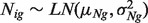and 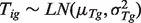where LN represents distribution because the transformed data were shown to empirically follow a normal distribution (Carvalho et al., 2007).

The fundamental challenge of deconvolution is how we predict T's, given that we observe the Y's and N's without previous information on the T's and π’s. If only a single sample were available, this would be an unsolvable problem, as both π's and T's are unknown. However, simultaneous analysis of several samples can teach us: to what extent a gene is component specific, in which component a gene is likely to be expressed more or less, and how variable a gene is across samples. These elements allow us to make predictions on the π's and T's. Note that the roles of tumor and normal tissues can be swapped, i.e. we can observe the pure tumor expression T's and make inference about the unobserved N's from the heterogeneous sample Y's. Another challenge lies in the distribution of Y, which does not follow a distribution when both N_ig and T_ig follow a distribution. With this in mind, our method mainly consists of two steps: (i) given the Y's and the distribution of the N's, we search for a set of that maximize the likelihood of observing Y; (ii) given the π's and the distributions of the T's and N's, we estimate an individual pair of (T, N) for each sample and each gene. Below, we describe these steps for specific data scenarios.

2.1 Data scenario 1: unmatched tumor and normal samples, without reference genes

This is a general and common data scenario. We observe 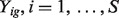and a set of unmatched observations of normal samples. We first obtain the sample mean and variance () under the distribution for the normal tissue samples. This allows us to initialize n_ig, which cannot be observed from the unmatched samples (see the Appendix for details). Unlike a mixture of normal distributions generating a normal distribution (for log-transformed data), the distribution of Y as a mixture of two distributions does not have a closed form. We, therefore, estimate and t_ig as follows.

1. Obtain an optimal set of along with using the Nelder–Mead procedure (Nelder and Mead, 1965). This set should maximize the likelihood for observing the expression levels Y's, i.e. 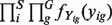(see the Appendix for details).

2. Given , we further deconvolve y_ig into n_ig and t_ig. The values of t_ig and n_ig are reconstituted gene expression levels of pure tumor and normal tissue corresponding to subject i and gene g. Given , we can write n_ig as a function of y_ig and t_ig. We search for a value of t_ig that is most likely to be presented given the LN distributions of N and T (see geometric illustration in Supplementary Fig. S1):

   (2)

   where is a density with corresponding mean μ and variance .

Our algorithm initializes n_ig and iterates (usually a couple of times) between Steps 1 and 2 (n_ig is updated using ), until the change in between two consecutive iterations is <1%.

2.2 Data scenario 2: matched tumor and normal samples, without reference genes

We do not need to initialize a known n_ig, and can replace Step 2 with

(3)

We estimate by following the same steps described in Section 2.1. The can have negative values for some genes, in which case we set t_ig at 0 and exclude these genes from the likelihood computation.

2.3 Data scenario 3: unmatched tumor and normal samples, with reference genes

We derive the tumor expression level distribution (with and ) for a reference gene set, as denoted by . Then under the linear relationship (1), we follow procedures as described in Section 2.1, except for the Nelder–Mead optimization procedure in Step 1. Instead, to estimate , we do the following:

(4)

where is a L₁ norm.

2.4 Data scenario 4: matched tumor and normal samples, with reference genes

This is a most desirable but uncommonly observed data scenario. We first estimate using Equation (4) given and for a set of reference genes, then estimate using Equation (3).

2.5 Methods for comparison

For comparison purposes, we implemented a linear model (LM) for the log-transformed data. This model estimates tumor proportions and gene expressions by assuming a normal distribution on the normal, tumor and mixed tissue samples. Following a similar procedure as in DeMix, we estimated associated parameters, as they maximize the likelihood of observing the -transformed expression values from the mixed tissue samples (see the Appendix for details). In addition, we present results based on a non-mixture model (NM), which ignores tumor heterogeneity ( for all tumor samples).

2.6 Uncertainty measure

We applied a standard bootstrap method (Efron, 1979) to estimate the uncertainty on the tumor proportion estimates . Given the set of genes used for deconvolution, e.g. all genes denoted by G or reference genes denoted by , we sampled these genes with replacement for m times (m = 50) and obtained a set of estimates for each experiment: . Then, we calculated the standard deviations of as standard errors.

3 RESULTS

3.1 Simulation

We used simulation to assess the performance of our approach in estimating unobserved tissue proportions and reconstituting unobserved tissue-specific expressions. Deconvolutions in matched designs with or without reference genes and in unmatched designs with reference genes are reported in the Supplementary Materials (Supplementary Figs S2–S4). Here, we present results from the unmatched design without reference genes (Section 2.1).

We simulated datasets as follows: 20 samples, 10 of pure A-type and 10 of mixed tissues. For the 10 mixed tissue samples, we assigned B-type tissue fractions, s, at evenly spaced values from 0.1 to 0.9. In each sample, we simulated expression levels for 2000 genes and randomly selected 25% (500 genes) to be differentially expressed (DE) when comparing A-type with B-type samples. We assumed the expression levels to follow distributions with mean and variance as follows. For A-type tissues, a vector consisting of means was generated independently from . For DE genes in B-type cell samples, the means of the A-type tissue samples were added by 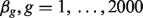, where we generated . For non-DE genes, s were sampled from . Across 10 pairs of A and B-type tissue samples, the sample-wise standard deviation at a given gene was set at 0.2. Then, we mixed the 10 A-type and B-type tissue sample expressions linearly at assigned proportions based on Equation (1). By doing so, we created 10 heterogeneous samples along with 10 observed A-type tissue samples. The 10 B-type tissue samples were hidden and used for validation. We repeated this procedure to generate 200 replicate datasets.

In Figure 1, we present results of the biases and mean-squared errors (MSEs) with respect to our estimation of B-type tissue proportion s. Compared with LM, DeMix resulted in substantially smaller biases and MSEs. LM performed worse at estimating proportions as the true proportion decreased. In contrast, DeMix performed well across all values of . This uniformity in performance is desirable because the actual tumor proportions will be unobserved in real data. As an example, at , we observed biases of 0.02 for DeMix and 0.28 (14-fold larger) for LM; at , the bias was 0.02 for both DeMix and LM.

Fig. 1.

Simulation results for data scenario 1. Shown are estimates of biases, MSEs and IRMSEs based on the DeMix and LM, for mixed samples at assigned B-type tissue proportions () varying from 0.1 to 0.9. For IRMSE, we also present results from the NM model

To evaluate how well DeMix reconstituted the B-type tissue expression level, we used an integrated relative mean-squared error (IRMSE) to quantify the discrepancy between the true expression (t_ig) and the estimated pure tissue expression () for sample i and gene g:

We estimated using DeMix, LM and NM, respectively. Figure 1 shows that our approach outperformed the LM and NM in estimating pure gene expressions. Again, as the actual B-type tissue proportion increased to a value close to 1, the LM and even the NM (no deconvolution) provided gene expression levels close to the truth. This suggests that DeMix provides the best improvement when analyzing heterogeneous samples with low to medium tumor proportions. Without knowledge of the true gene expression levels, however, we cannot obtain information on tumor proportions a priori, which vary across samples. When the true B-type tissue proportion was low, the LM performed better than the NM, but at a degree that was not comparable with the performance of DeMix. The monotonic trend in the bias from the LM can be explained by our simulation settings. Here, we assume all differentially expressed genes were overexpressed in the tumor tissue as compared with the normal tissue. When all tumor tissue expressions are underexpressed compared with the normal tissue expressions, however, this trend can be reversed (Supplementary Tables S2 and S3).

3.2 Data example

To validate our method using real data under data scenario 1 (Section 2.1), we analyzed four public gene expression datasets, which are generated by artificially mixing tissues at varying proportions.

• We downloaded dataset GSE19830 from the GEO website (http://www.ncbi.nlm.nih.gov/geo/). This dataset was originally generated from rat microarray experiments (Shen-Orr et al., 2010) with Affymetrix Rat Genome 230 2.0 Arrays and consists of 12 mixed samples of liver and brain tissues in four proportions (Supplementary Table S1) and 3 samples each from pure liver and brain tissues.

• We obtained two datasets within GSE5350 from GEO: Affymetrix Human Genome U133 Plus 2.0 arrays generated by the MicroArray Quality Control (MAQC) project (MAQC Consortium, 2006). The RNA samples consist of isolated 100% Stratagene Universal Human Reference RNA (A) and 100% Ambion Human Brain Reference RNA (B) and their mixtures in varying proportions. Ten samples were processed using Affymetrix platform (Affymetric Inc., 2012), and 10 samples were processed using Illumina platform (Illumina Inc., 2009) denoted as MAQC sites 1 and 3, respectively.

• We downloaded Affymetrix array data from http://www.affymetrix.com/support/technical/sample_data/gene_1_0_array_data.affx. This dataset consists of samples with varying proportions of human brain and heart tissues. We selected 18 samples with proportion ratios of 0/100% (three samples), 25%/75% (three samples), 50%/50% (six samples), 75%/25% (three samples) and 100%/0 (three samples).

To summarize the probe intensities in all datasets, we used the robust multi-array averaging (RMA) procedure (Irizarry et al., 2003), as implemented in R (R Development Core Team, 2009) and bioconductor (http://www.bioconductor.org). To maintain computational efficiency and remove probes with high background noise, we selected a subset of genes to be analyzed by DeMix. We required the mean expression levels of these genes in pure normal tissue samples to be in the upper quartile of the expression levels of all genes. This provided us with 7000–14 000 probesets across all datasets.

With pre-processed raw measured data, we confirmed that assuming a linear mixture on the data before they are log-transformed is appropriate, as compared with assuming it on the log-transformed data. This can be done when we know and Y, from which we derive . Specifically, in dataset GSE19830, we compared the differences in transcript abundances between the pure liver and brain tissues (T–N), with differences between the mixed and brain tissues (Y- N), both at the original scale (Fig. 2a) and at the scale (Fig. 2b). The linear relationship AX = B fits well with the raw measured data, with a few deviations in genes at extreme values, e.g. at . In the log-scale data, however, the linearity assumption does not hold when the abundance ratio between two tissues is >2-fold.

Fig. 2.

Scatter plots of transcript abundance in mixed-sample expressions minus brain expressions (Y–N) versus pure liver expressions minus pure brain expressions (T–N) at two different mixing rates for (a) log-transformed data; (b) raw measured data

First, we evaluated how well DeMix estimated tissue proportions in these datasets (Fig. 3). Without using previous knowledge of tissue-specific expression from both components of the mixture, as in other methods (Shen-Orr et al., 2010), DeMix correctly estimated the unknown tissue proportions with a correlation coefficient, r, of 0.98. In contrast, LM consistently overestimated the tissue proportions, likely because of the concavity property of log functions, as explained by Zhong and Liu (2011). Of 47 samples, all estimates from GSE19830 and MAQC site 1 presented 95% confidence intervals that included the truth, or less often, with one boundary 1–2% away from the truth (see also Supplementary Table S1). We observed three samples from Affymetrix and two samples from MAQC site 3 that presented overestimated proportions. The first overestimation was likely caused by deviation from the linearity assumption, which we diagnosed using scatter plots of (T–N) versus (Y–N) (Supplementary Fig. S5). With the normalized raw measured data, we still observed a curvature in the three samples, with many data points at both extremes of the (Y–N) values unevenly distributed on top of an expected line of 25% (the true proportion). The second overestimation was likely caused by issues in data quality. We compared the MA plots of all five samples generated at the same proportion of 25% for the MAQC site 3 data (Supplementary Fig. S6). We observed larger variations in probe intensities for samples 1 and 3 compared with those of the other three samples (respective inter-quartile ranges of 0.19 and 0.18 versus 0.06, 0.08 and 0.05). We obtained similar results when analyzing the four datasets with probesets presenting expression levels >2⁶ in the normal samples (35–49% of all probesets, Supplementary Fig. S7). We observed overestimation in tissue proportions in the same five samples.

Fig. 3.

Estimation of proportions of hidden tissues from four available data sources. MAQC1: MAQC site 1, MAQC3: MAQC site 3, AFFY:Affymetrix, and GSE19830. (a) Estimated tissue proportions versus true proportions; black represents the DeMix estimates; gray represents LM estimates. (b) Estimated 95% confidence intervals of 's; solid lines correspond to true π's

Next, we examined how well DeMix reconstituted pure tissue-type expressions at four different proportions using the GSE19830 data as an example. As shown in a heatmap (Fig. 4a), DeMix removed mixed-in gene expressions from brain tissue samples at different mixture proportions. It provided individual gene expression levels from pure liver tissue that are more homogeneous across 12 samples than they were before deconvolution, and more similar to the actual gene expressions in pure liver tissue. Figure 4b shows the estimated expressions from pure liver tissue are highly correlated with the true expressions (correlation coefficient ). Within each sample, we achieved greater accuracy when the gene expression levels were high for pure samples, as low expression levels may be overrepresented by a high level of background noise. We obtained similar results from the other three datasets, and lower correlation coefficients in samples where the proportion estimates were significantly different from the truth (Supplementary Fig. S8).

Fig. 4.

Estimation of gene expression values of hidden tissues from GSE19830. (a) Heat map of expression values from selected genes across samples. The proportions of liver tissue are shown at the bottom. A total of 1323 genes were randomly selected. The samples, left to right, are 3 pure brain samples (observed), 12 liver-brain mixed samples (observed), 12 deconvolved liver samples (unobserved; estimated) and 3 pure liver samples (unobserved; used for comparison). (b) Scatter plots comparing deconvolved mean liver tissue expression levels with observed mean pure liver expression levels at four different mixture proportions of brain tissues

Finally, we illustrated the use of DeMix in finding DE genes, again using the GSE19830 dataset as an example. Figure 5 shows the number of significant genes (found by a two-sample t-test) between liver and brain tissue samples at varying cut-offs of the P-values (Bonferroni corrected). At an initial cut-off of 0.05, DeMix-based deconvolution found 4774 DE genes, which was ∼1.3 times more than those found by LM (3598) and 9 times more than those found by NM (523). We also directly compared the observed pure brain and pure liver tissue samples. Given a relatively small sample size (3 versus 3, as compared to 12 versus 3 from mixed samples), we found only 1900 genes, 2.5 times fewer than the amount found with DeMix. Even though these 1900 genes largely overlapped with the 4774 genes found by DeMix, the different sample size, and hence the different statistical power, prohibited us from using these 1900 genes as truth. The issue of small sample size is also supported by an observation that at a P-value cut-off of ≤0.001, the NM (not considering heterogeneity) yielded a higher number of DE genes than the ‘pure’ samples. As we lowered the cut-off on P-value, we found more DE genes with DeMix. We tested the homogeneity among 12 deconvolved samples by performing two-sample t-tests between six randomly selected deconvolved samples against the remaining six samples. At a P-value cut-off of 0.05, we did not find any significant DE genes. These results suggest that DeMix-based deconvolution is able to make mean differences more distinct between two tissue samples and reduces variances across all single tissue samples (Fig. 4a), both of which contributed to increasing the power of detecting DE genes.

Fig. 5.

Detection of DE genes. Total number of identified differentially expressed genes at varying P-value cut-offs (Bonferroni-corrected), using different models. The third curve from the top corresponds to comparison between the three pure brain and the three pure liver tissue samples

4 CONCLUSION

We have presented a novel statistical method, DeMix, for computational dissection of gene expression levels from mixed tissue samples, and in particular, for microarray data generated from cancer patient samples. Our method addresses three existing problems for in silico dissection: (i) model-based analysis of raw measured data that follow a instead of a normal distribution; (ii) estimation of both tissue proportions and tissue-specific expression levels; and (iii) reconstitution of patient-specific gene expressions. We also provide uncertainty measures on estimated tissue proportions. DeMix provides practical solutions by requiring knowledge of gene expression of one tissue type, which does not have to be matched, i.e. derived from the same sample. Our solutions vary according to data scenarios, to take advantage of all the available information. Both simulation studies and analysis of actual data highlight the importance of following a linear mixture of gene expression levels on data before they are log-transformed, for which DeMix is the first method to do so. Our validation study showed that DeMix performs accurately on expression data generated from both Affymetrix and Illumina platforms. Our method can be applied to analyzing newly generated expression data from biomarker studies, as well as to re-analyzing data generated from previous studies.

Our method is useful when there is little information on gene expression levels in one of the mixing components, and at the same time the mixing proportions, which could be obtained from other sources such as pathologist estimates or from DNA copy number data (Yau et al., 2010), are not available. We do not require knowledge of reference genes. However, when such knowledge is available, we have provided an alternative solution to take advantage of the information. Even though our algorithm requires a minimum of one gene as a reference gene, we recommend using at least 5–10 genes to alleviate the potential influence from outliers and to identify an optimal set of πs. DeMix uses expression levels from thousands of genes to estimate each π and is, therefore, robust to perturbations in the expression of a minority of genes, arising from interaction with surrounding tumor cells. DeMix can also use a list of selected genes that are not affected by the tumor, when available, for the estimation of proportions. If cell proportions are estimated reliably, they can also be used to estimate mean expression levels in both normal and tumor tissues for potentially perturbed genes, based on the linear relationship on raw measured data. When reference genes are considered, DeMix performed similarly or better than PERT (Qiao et al., 2012) in estimating tissue proportions with our validation data (Supplementary Figs S9 and S10).

Our estimation procedure under matched or unmatched samples with reference genes is computationally efficient. On a PC with a 2.2 GHz Intel Core I7 processor, the computation of our simulation data consisting of 20 matched samples and 2000 genes in each sample takes ∼1 s. In contrast, it takes ∼10 min to complete the computation of the same data without knowledge of any reference genes. We used the Nelder–Mead optimization procedure that includes a numerical integration of the joint density, which may explain this substantial increase in computation time. DeMix takes a two-stage approach by first estimating the 's and then estimating the means and variances of gene expressions based on the 's. A joint model that estimates all parameters simultaneously will be able to further incorporate the uncertainty measure of the tissue proportions. However, the estimation step from such a model can be computationally intensive and may not be suitable for the analysis of high-throughput data.

We identified a few considerations for the deconvolution of microarray data. First, the assumed linear mixture of data before they are log-transformed may not perfectly hold for some samples, e.g. samples 1 to 3 from the Affymetrix data, and for some genes, e.g. those with extreme expression values such as <2⁴ or >. Second, our estimation method is based specifically on distributions of the raw measured data for each mixture component. When this assumption is violated, a deterioration of accuracy is to be expected. Third, microarray technology has inherent limitations, such as high background noise and inconsistent gene expressions across experiments. Screening out genes with low expression levels and accounting for batch effects must be tackled before deconvolution. We found scale normalization using MAS5 can obscure the actual linear mixture of expression levels, on which the downstream deconvolution is based. Summarization using RMA, together with quantile normalization, seemed to retain our linearity assumption of the raw measured data most of the time.

Our model assumes that a mixed sample consists of at most two cellular compartments: normal and tumor, and that the distributional parameters of normal cells can be estimated from other available data. These assumptions seem to us to be a logical place to begin, but there remain important situations where more complex modeling may be needed. First, we assume pure normal samples to be representative of the normal tissues in the mixture samples, allowing for estimation of sample-specific expression values. This assumption can be violated as there are sometimes perturbations of gene expression levels in tumor–stromal interactions, as previously discussed. Second, both normal and tumor tissues may in turn consist of different cell types, with different transcriptional activity, and represented in proportions that can be variable across samples. This has been studied in Qiao et al. (2012), which used reference profiles from all cell types. Extensions of our model to deconvolution of more than two mixture components can address this issue without requiring reference profiles from all mixing components and can be done with a more computationally efficient density integration and optimization procedure. Currently, to identify 's, we assume a roughly stable composition of one or multiple cell types within each tissue component. With data from real tissue samples, it is necessary to evaluate the extent to which this assumption is valid. The variation in the composition of multiple cell types from sample to sample will be captured by the variance of the distribution of expression levels within each tissue, which is estimated based on the data. When there exist multiple tumor subtypes, our method should be applied separately to samples that belong to the same subtype.

REFERENCES

- Abbas AR, et al. Deconvolution of blood microarray data identifies cellular activation patterns in systemic lupus erythematosus. PLoS One. 2009;4:e6098. doi: 10.1371/journal.pone.0006098. [DOI] [PMC free article] [PubMed] [Google Scholar]
- Carvalho B, et al. Exploration, normalization, and genotype calls of high-density oligonucleotide SNP array data. Biostatistics. 2007;8:485–499. doi: 10.1093/biostatistics/kxl042. [DOI] [PubMed] [Google Scholar]
- Clarke J, et al. Statistical expression deconvolution from mixed tissue samples. Bioinformatics. 2010;26:1043–1049. doi: 10.1093/bioinformatics/btq097. [DOI] [PMC free article] [PubMed] [Google Scholar]
- Efron B. Bootstrap methods: Another look at the jackknife. Ann. Stat. 1979;7:1–26. [Google Scholar]
- Emmert-Buck MR, et al. Laser capture microdissection. Science. 1996;274:998–1001. doi: 10.1126/science.274.5289.998. [DOI] [PubMed] [Google Scholar]
- Erkkilä T, et al. Probabilistic analysis of gene expression measurements from heterogeneous tissues. Bioinformatics. 2010;26:2571–2577. doi: 10.1093/bioinformatics/btq406. [DOI] [PMC free article] [PubMed] [Google Scholar]
- Ghosh D. Mixture models for assessing differential expression in complex tissues using microarray data. Bioinformatics. 2004;20:1663–1669. doi: 10.1093/bioinformatics/bth139. [DOI] [PubMed] [Google Scholar]
- Gosink MM, et al. Electronically subtracting expression patterns from a mixed cell population. Bioinformatics. 2007;23:3328–3334. doi: 10.1093/bioinformatics/btm508. [DOI] [PubMed] [Google Scholar]
- Irizarry RA, et al. Exploration, normalization, and summaries of high density oligonucleotide array probe level data. Biostatistics. 2003;4:249–264. doi: 10.1093/biostatistics/4.2.249. [DOI] [PubMed] [Google Scholar]
- Lu P, et al. Expression deconvolution: a reinterpretation of DNA microarray data reveals dynamic changes in cell populations. Proc. Natl. Acad. Sci. USA. 2003;100:10370–10375. doi: 10.1073/pnas.1832361100. [DOI] [PMC free article] [PubMed] [Google Scholar]
- MAQC Consortium. The microarray quality control (MAQC) project shows inter- and intraplatform reproducibility of gene expression measurements. Nat. Biotechnol. 2006;24:1151–1161. doi: 10.1038/nbt1239. [DOI] [PMC free article] [PubMed] [Google Scholar]
- Nelder JA, Mead R. A simplex method for function minimization. Comput. J. 1965;7:308–313. [Google Scholar]
- Qiao W, et al. PERT: A method for expression deconvolution of human blood samples from varied microenvironmental and developmental conditions. PLoS Comput. Biol. 2012;8:e1002838. doi: 10.1371/journal.pcbi.1002838. [DOI] [PMC free article] [PubMed] [Google Scholar]
- R Development Core Team. R Foundation for Statistical Computing. Vienna, Austria: 2009. R: a Language and Environment for Statistical Computing. ISBN 3-900051-07-0. [Google Scholar]
- Shen-Orr SS, et al. Cell type-specific gene expression differences in complex tissues. Nat. Methods. 2010;7:287–289. doi: 10.1038/nmeth.1439. [DOI] [PMC free article] [PubMed] [Google Scholar]
- Stuart RO, et al. In silico dissection of cell-type-associated patterns of gene expression in prostate cancer. Proc. Natl Acad. Sci. USA. 2004;101:615–620. doi: 10.1073/pnas.2536479100. [DOI] [PMC free article] [PubMed] [Google Scholar]
- Tothill RC, et al. An expression-based site of origin diagnostic method designed for clinical application to cancer of unknown origin. Cancer Res. 2005;65:4031–4040. doi: 10.1158/0008-5472.CAN-04-3617. [DOI] [PubMed] [Google Scholar]
- Tsao AS, et al. Clinical outcomes and biomarker profiles of elderly pretreated NSCLC patients from the BATTLE trial. J. Thorac. Oncol. 2012;11:1645–1652. doi: 10.1097/JTO.0b013e31826910ff. [DOI] [PMC free article] [PubMed] [Google Scholar]
- Venet D, et al. Separation of samples into their constituents using gene expression data. Bioinformatics. 2001;17:S279–S287. doi: 10.1093/bioinformatics/17.suppl_1.s279. [DOI] [PubMed] [Google Scholar]
- Wang M, et al. Computational expression deconvolution in a complex mammalian organ. BMC Bioinformatics. 2006;7:328. doi: 10.1186/1471-2105-7-328. [DOI] [PMC free article] [PubMed] [Google Scholar]
- Yau C, et al. A statistical approach for detecting genomic aberrations in heterogeneous tumor samples from single nucleotide polymorphism genotyping data. Genome Biol. 2010;11:R32. doi: 10.1186/gb-2010-11-9-r92. [DOI] [PMC free article] [PubMed] [Google Scholar]
- Zhong Y, Liu Z. Gene expression deconvolution in linear space. Nat. Methods. 2011;9:8–9. doi: 10.1038/nmeth.1830. [DOI] [PubMed] [Google Scholar]
Associated Data
This section collects any data citations, data availability statements, or supplementary materials included in this article.