Measurement of SAR-induced temperature increase in a phantom and in vivo with comparison to numerical simulation

Abstract

Purpose

Compare numerically-simulated and experimentally-measured temperature increase due to Specific energy Absorption Rate (SAR) from radiofrequency fields.

Methods

Temperature increase induced in both a phantom and in the human forearm when driving an adjacent circular surface coil was mapped using the proton resonance frequency shift technique of Magnetic Resonance (MR) thermography. The phantom and forearm were also modeled from MR image data, and both SAR and temperature change as induced by the same coil were simulated numerically.

Results

The simulated and measured temperature increase distributions were generally in good agreement for the phantom. The relative distributions for the human forearm were very similar, with the simulations giving maximum temperature increase about 25% higher than measured.

Conclusion

Although a number of parameters and uncertainties are involved, it should be possible to use numerical simulations to produce reasonably accurate and conservative estimates of temperature distribution to ensure safety in MR imaging.

INTRODUCTION

To ensure patient safety and comfort during Magnetic Resonance Imaging (MRI), measures are taken to limit both the total radiofrequency (RF) energy absorbed by the entire human body (whole body Specific energy Absorption Rate, or SAR_WB) or a region thereof (e.g., SAR_head), and the maximum energy absorbed in any local region (maximum local Specific energy Absorption Rate, or maximum SAR_local), often averaged over a 10-gram region (1). Estimates of SAR_WB can be based on measurements of total patient mass and total RF power delivered to the patient. Estimates of maximum SAR_local typically rely both on these measureable quantities and on numerical simulations of the distribution of SAR throughout the subject (2). For example, numerical simulations of maximum SAR_local/SAR_WB can be multiplied by measured SAR_WB to produce an estimate of SARlocal in the subject. Accurate estimates of SAR_local when using parallel transmission also require consideration of the magnitude and phase at which the individual coils are driven (3-7).

Some investigators have additionally demonstrated various approaches to simulating temperature under the influence of SAR during MRI (8-14). Although it is generally recognized that tissue temperature is a more relevant quantity than SAR for relating to safety, SAR is seen to be more readily and accurately ascertained by directly measureable quantities during MRI. While this is certainly true for SAR_WB, numerical calculations of SAR_local throughout the body are limited by (among other things) dependence on anatomical variation (15-18), such as limited similarity between the models used in simulation and the morphology of the specific human subject. Some recent studies have shown, however, that simulations of temperature increase vary less with anatomical variation than does SAR (16), giving simulation of temperature another potential advantage (in addition to higher relevance to safety) over simulation of SAR alone.

A third potential advantage of simulating temperature over simulating SAR alone is that temperature, or at least temperature increase, can be mapped in tissue using methods of Magnetic Resonance (MR) thermography and used to validate the accuracy of the simulation technique. The Proton Resonance Frequency (PRF) shift technique of MR thermography (19) has been used previously to map temperature change in vivo due to intentional heating in ablation with ultrasound (20), laser (21), and RF energy (22), and in hyperthermia with RF energy (23). It has also been used in unperfused phantoms to validate numerical calculation of SAR (24-27), but temperature distribution in vivo is also largely a function of tissue perfusion, which is typically considered in simulations of temperature.

Here we use PRF shift MR thermography in a phantom and in the human forearm to assess temperature increase induced by driving an adjacent circular surface coil, and we compare to numerical simulations of temperature increase in models created from MRI data from the same phantom and forearm.

METHODS

We performed simulations of temperature and measurements of temperature increase both in a phantom and in vivo. Below, procedures for all calculations and experiments are described.

Experimental mapping of temperature increase in an agar-gel phantom

Using the PRF-shift method of MR thermometry, we imaged the temperature change (ΔT) in a rectangular-shaped agar-gel phantom (Figure 1, left). Heating was accomplished using a home-built one-loop coil (diameter = 80 mm, Figure 1, center) connected to an RF power amplifier (LA200UELP, Kalmus, WA, USA) located outside of the MR scan room. The input to the amplifier was a continuous-wave 165 MHz signal produced by a frequency synthesizer (PTS 200, PTS, MA, USA) (28). The coil used for heating was tuned to a different frequency from the Larmor frequency (123.2 MHz) to avoid coupling between the heating and imaging coils. The ratio of the quality factor when the coil was loaded and unloaded was measured as 0.05, indicating that approximately 95% of the RF power delivered to the coil was dissipated in the phantom or forearm (29). The RF power delivered to the heating coil was monitored using a directional coupler (C8212-10, Werlatone, Inc., NY, USA), time-averaged RF power sensor (U2001A, Agilent Technology, Inc.), and RF power meter (N9912A, Agilent Technology, Inc.) during the MR temperature mapping. Between the directional coupler and the coil was a 5m cable with 1dB attenuation, as determined with a network analyzer (HP 4195A, Hewlett Packard, Inc.).

Figure 1.

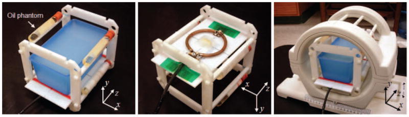
Phantom and frame with the agar-gel phantom and four oil phantoms (left), RF induction-heating coil attached to bottom of frame (middle), and one-channel Tx/Rx extremity RF coil loaded with phantoms and frame (right).

The agar-gel phantom consisted of a gel (10g/L NaCl, 1g/L CuSO₄, and 7g/L agar in distilled water) in a 2 mm-thick plastic container. The gel phantom had width, height, and depth of 78, 68, and 142 mm, respectively (width and depth measured at surface adjacent coil). Mass density (ρ) of the phantom was measured as 1021 kg/m³. The electrical conductivity (σ) and relative permittivity (ε_r) of the phantom were 2.97 S/m and 74.15 respectively, as measured with an impedance/material analyzer (E4991A, Agilent Technology, Inc.) and dielectric probe kit (85070D, Agilent Technology, Inc.) at 165 MHz. The phantom was separated from the heating coil by a 4 mm-thick Teflon plate. The coil was matched to -30 dB when loaded with the phantom.

To accomplish imaging, the phantom and heating coil were positioned a single-channel Tx/Rx CP extremity coil (Figure 1, right) within a Siemens Tim Trio 3 T MRI system (Erlangen, Germany). Four cylindrical oil phantoms (diameter=15 mm) were positioned about the phantom (Figure 1, left) for tracking and correction of temporally/spatially varying phase drift during the heating period (30, 31). An initial phase map was collected using a gradient-echo sequence on the center axial plane (TR/TE 30/10 ms, 3 slices, 10 mm slice thickness, FOV 150 × 150 mm², matrix size 256 × 256, flip angle 40 degrees, 4 averages, 92.2 second scan time). Then 42.5 W of RF power was delivered to the heating coil for 2 minutes (i.e., 40.4 W was dissipated in the phantom). Immediately after heating, a second phase map was collected with the same scan parameters with the first phase map but with no averaging to minimize the cooling during scanning. The scan time of the second phase map was 23 seconds.

Considering the phase drift corrections, the temperature change (ΔT) maps in the phantom were calculated as

$$\mathrm{\Delta T}=\frac{\mathrm{\Delta }\varphi -\mathrm{\Delta }{\varphi }_{\mathrm{drift}}}{\alpha \times \gamma \times {\mathrm{B}}_0\times \mathrm{TE}}$$ [1]

where Δϕ is measured phase change, Δϕ_drift is phase change due to system phase drift, α is the PRF shift coefficient for water (-0.01 ppm/°C), γ is the gyromagnetic ratio (42.58 MHz/T), B₀ is the main magnetic field strength, and TE is echo time. Maps of Δϕ_drift were created by averaging phase information from the phase change over 3×3 pixel regions in each oil phantom and interpolating across the image region from these four averaged values.

Numerical simulation of SAR and temperature for the agar-gel phantom

A numerical model of the phantom (Figure 2) was created by manually segmenting a series of axial images (54 slices with 3 mm thickness, 0 mm gap) acquired after the heating experiment. The model was assigned the same σ, ε_r, and ρ as were measured in the experimental phantom. Models of the plastic container, Teflon plate, and coil were added manually. The coil model was tuned and driven at a single location, as in experiment. The final simulation space consisted of 118 × 117 × 198 cells having resolution 1.17 × 1.17 × 1 mm³. Numerical field simulations were performed using commercially-available software (XFdtd, Remcom, Inc.) and a graphics processing unit (Tesla C1060, NVIDIA, Inc.). After the field simulation, the SAR was calibrated by scaling the dissipated power in the phantom to match that measured in the experiment. The physical properties assigned various materials in the model are summarized in Table 1.

Figure 2.

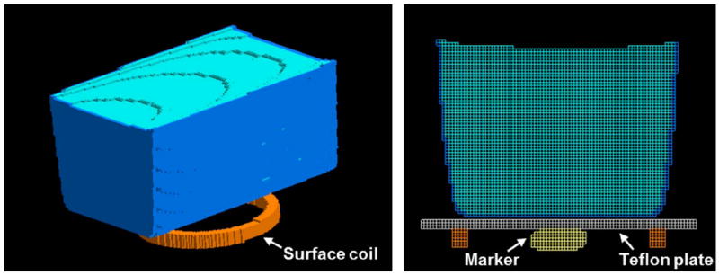
Phantom mesh model with the RF induction-heating coil (left; Teflon plate is not shown for better visualization) and center plane of the phantom mesh model (right). Small oval shaped object is a marker placed at the coil center and imaged in experiment to aid in accurate modeling.

Table 1.

Physical properties of tissues and materials used in simulations: Electrical conductivity (σ, S/m), relative electric permittivity (ε_r), mass density (ρ, kg/m³), perfusion by blood (w_b, mL/100g/min), heat capacity (C, J/kg/°C), thermal conductivity (k, W/m/°C), and metabolic heat generation (Q, W/m³).

Tissue	σ	εr	ρ	wb	C	k	Q
Agar-gel	2.97	74.15	1021	0	4200	0.498	0
Polypropylene	0	2.1	2200	0	1925	0.16	0
Teflon	0	2.1	2200	0	1050	0.16	0
Skin	0.551	59.53	1125	12	3150	0.343	1125
Tendon	0.508	50.31	1151	5	3500	0.498	758
Fat	0.038	5.81	943	2.8	2300	0.23	302
Cortical bone	0.071	14.26	1850	1.4	1300	0.35	0
Cancellous bone	0.188	25.17	1080	3	2238	0.36	0
Blood	1.266	70.31	1057	100	3600	0.51	0
Muscle	0.732	61.52	1070	5	3500	0.59	480

The temperature distribution throughout space and time was then determined using a finite difference implementation (8) of the Pennes bioheat equation (32),

$$\mathrm{\rho c}\frac{\mathrm{dT}}{\mathrm{dt}}=▽(\mathrm{k}▽\mathrm{T})+[­{\mathrm{\rho }}_{\mathrm{blood}}{\mathrm{w}}_{\mathrm{b}}{\mathrm{c}}_{\mathrm{b}}(\mathrm{T}­{\mathrm{T}}_{\mathrm{core}})]+{\mathrm{Q}}_{\mathrm{m}}+\mathrm{SAR\rho }$$ [2]

where ρ is material density, c is heat capacity, k is thermal conductivity, w_b is perfusion by blood, c_b is heat capacity of blood, and Q_m is heat generated by metabolism. Detailed electrical and thermal property settings are shown in Table 1. Initial temperature distribution was determined by iteratively solving equation 2 without any SAR until the temperature reached an equilibrium state (T_EQ). Starting from this state, the temperature distribution after heating (T_SAR) was recorded after 139.2 seconds (120 seconds of heating plus 19.2 seconds of cooling – the time required to reach the center of k-space during acquisition of the second phase map). Finally, the temperature change maps in the phantom were calculated by subtracting T_EQ from T_SAR. More detailed description and validation of the finite difference implementation of the Pennes bioheat equation is given elsewhere (8).

Experimental mapping of temperature increase in human forearm

Temperature maps of the in vivo human forearm were acquired in the same overall manner as in the phantom study, including power measurement with a directional coupler and power sensor. The inductive heating coil was positioned beneath the forearm as shown in Figure 3. The heating coil was matched to -26 dB at 165 MHz when loaded in the magnet. We acquired the first phase map of the forearm (TR/TE 100/10 ms, flip angle 40 degrees, FOV 160×160 mm², matrix size 128×128, slice thickness 10 mm, 4 averages, imaging time 51.2 seconds) before applying 33 W of RF power to the heating coil for 2 minutes. The RF power delivered to the forearm was 31.4 W, considering the ratio of the quality factor when the coil was loaded and unloaded (0.05) and the 1dB attenuation from the cable between the directional coupler and the coil. The second phase map was acquired immediately after the 2 minute heating period. The sequence for the second phase map was identical to the that of first phase map scan but with no averaging so that the acquisition time was 12.8 seconds. The phase drift during the RF heating period was monitored and corrected using the four oil phantoms at each corner of axial plane as for the phantom. We assumed -0.01 ppm/°C for the chemical shift coefficient to temperature changes (α) in this in vivo forearm temperature mapping. All procedures were performed with informed consent of the subject and in compliance with our institutional regulations on human subjects research.

Figure 3.

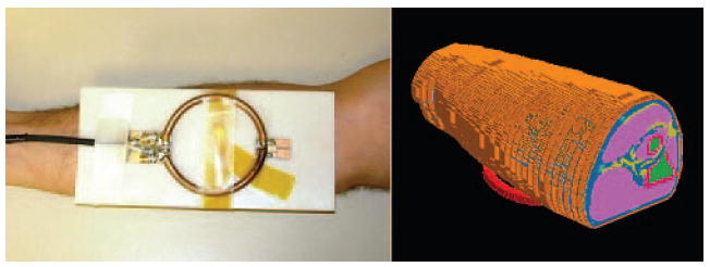
Surface coil against forearm for experiment (left) and in simulation (right).

Numerical simulation of SAR and temperature for in vivo forearm

A numerical model of the forearm (Figure 3) was created by manually segmenting MR images (multi-slice fast spin echo with 6 echoes per TR, TR/TE = 700/11 ms, FOV 160×160 mm², matrix size 384×384, 32 slices, 2 averages) acquired before the heating experiment. The resolution of the model was 0.83×0.83×1 mm³ and the number of cells in the model was about 4.9×10⁶ (172×143×199). A model of the heating coil was tuned and excited with one current source (1 A) for 10 periods at 165 MHz. The magnetic field at the center of forearm model was monitored to ensure the field calculation reached steady state, defined as when the variation in field magnitudes in successive periods changed by less than 1%. The volume of SAR data was then scaled so that the total dissipated power matched that in the experiment (31.4 W). The SAR volume data was then utilized in the numerical temperature simulation as in the phantom study.

For temperature simulation of the in vivo forearm, tissue perfusion rate (w_b) was a function of local temperature such that (33)

$${\mathrm{w}}_{\mathrm{b}}(i,j,k)=\{\begin{array}{cc}{\mathrm{w}}_{\mathrm{b}0}(i,j,k)& \mathrm{T}(i,j,k)\le 39°\mathrm{C}\\ {\mathrm{w}}_{\mathrm{b}0}(i,j,k)[1+{\mathrm{S}}_{\mathrm{B}}(\mathrm{T}(i,j,k)­39)],& 39°\mathrm{C}<\mathrm{T}(i,j,k)<44°\mathrm{C}\\ {\mathrm{w}}_{\mathrm{b}0}(i,j,k)(1+5{\mathrm{S}}_{\mathrm{B}})& \mathrm{T}(i,j,k)\ge 44°\mathrm{C}\end{array}$$ [3]

where T(i,j,k) is the local temperature at location (i,j,k), and S_B is a coefficient set equal to 0.8/°C (34). With this model (34) the local rate of perfusion, w_b, remains at its (initial) baseline level (w_b0) until the local temperature exceeds 39 °C. Between 39 °C and 44 °C, w_b increases linearly from w_b0 to its maximum value of 5 times w_b0. This model was initially developed to approximate experimental observations (35). For this numerical temperature simulation, the heating and cooling periods were 120 and 6.5 seconds, respectively. The physical properties assigned the various tissues and materials in the model were acquired from the literature (8, 33-37) and are summarized in Table 1.

To explore the sensitivity of the simulated maximum ΔT to uncertainty in the various physical parameters in Eq. 2, we also performed a series of simulations where these parameters were, one at a time, increased above their values in Table 1 by 10% throughout the forearm model.

RESULTS

The unaveraged SAR [W/kg], numerically simulated temperature, and PRF-based experimental temperature maps on the center slice of the agar-gel phantom are shown in the first row of Figure 4. Because the slice thickness of the temperature simulation and the PRF temperature maps were 1 and 10 mm, respectively, 10 slices of numerical temperature maps were averaged for comparison with experiment. Overall temperature patterns of both maps in the phantom are in fairly good agreement. In the region of largest disagreement (yellow arrow), the maximum temperature in the experimental temperature map is about 12% lower than that in the simulation. The asymmetry in experiment compared to simulation may be due to slight difference in positioning of the heating coil between the simulation and experiment. Simulated and measured values of maximum ΔT (13.66 and 13.70 °C, respectively) were in very good agreement (less than 1 % difference). The maximum ΔT was located at the bottom left in both simulation and experiment.

Figure 4.

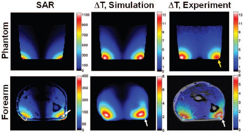
Simulated unaveraged SAR [W/kg] map (left column), simulated temperature increase [°C] (center column), and experimentally-measured PRF temperature increase [°C] (right column) for the agar-gel phantom (top row), and the in vivo forearm (bottom row). Yellow arrow indicates region of highest disagreement between experiment and simulation in phantom. White arrow indicates blood vessel having high SAR but only moderate temperature increase in forearm. The plane shown passes through the center of the coil and is transverse to the long axis of the phantom or forearm.

The unaveraged SAR map in the forearm model is given at the bottom left of Figure 4. As the white arrow indicates, the maximum local SAR is located in a blood vessel, since the blood vessel was close to the heating coil and the electric conductivity of blood is approximately three times higher than the surrounding tissues (skin, fat, muscle, etc.). Due to the flow of blood in the vessel (simulated as a nominally high perfusion rate in blood), this locally high SAR does not result in a locally high temperature. A smaller temperature increase in the blood vessel than in the nearby muscle is seen in both simulation and experiment. The overall temperature change patterns between the numerically simulated and the PRF temperature map of forearm are similar, but the maximum temperature change in experiment (6.00 °C) is 25% lower than that in simulation (8.02 °C). The maximum temperature increase at the ends of the model (at surfaces resulting from truncation of arm model) was 0.091 °C, indicating that only a minor effect of truncation should be present. To allow for better direct comparison in simulation and experiment in the regions of greatest interest, line plots of ΔT through the high-temperature regions in each case are given in Figure 5. To illustrate the importance of phase correction in calculating ΔT in experiment, the apparent temperature change due only to phase drift (without heating) that would be measured if uncorrected for is shown for the human forearm in Fig. 6.

Figure 5.

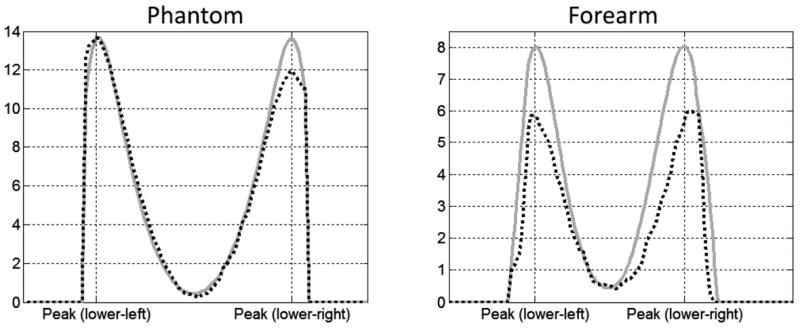
Temperature increase (°C) along lines passing through maxima in simulation (solid gray lines) and experiment (dotted black lines) for both the phantom (left) and forearm (right).

Figure 6.

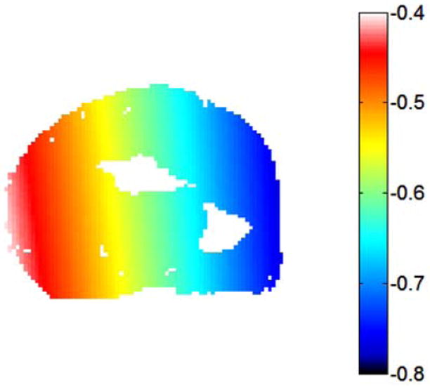
The additional temperature change (°C) that would be apparent due to phase drift in the forearm if not corrected. This potential contribution to the temperature map was removed by subtracting a phase drift distribution measured with the oil phantoms from the experimental phase maps.

The variation in simulated maximum ΔT due to a 10% increase of different physical parameters is given in Table 2. These values show the sensitivity of maximum ΔT to uncertainty of these parameters in the case simulated.

Table 2.

Variation in simulated maximum ΔT due to 10% increase in various physical parameters. Maximum ΔT in original simulation is 8.02 °C.

Parameter increased by 10%	C	k	Q	ρ	wb	σ	εr
Resulting change in max. ΔT (°C)	-0.55	-0.15	0.00	-0.57	-0.07	0.12	-0.02
Percent change in max. ΔT	-6.9%	-1.9%	0%	-7.1%	0.87%	1.5%	0.25%

DISCUSSION

In recent years, the use of numerical methods to predict SAR distributions has become very prevalent. By comparison, calculation of temperature is relatively rare. Damage to tissue is more directly related to temperature over time than to SAR, and can thus be expressed as a “thermal dose,” in a variety of ways (38, 39). It is possible that future regulatory guidelines for MRI will incorporate a sense of thermal dose, rather than just maximum temperature, into limits on RF exposure (1), giving impetus for increasingly meaningful predictions of RF safety. While the in vivo study presented here is limited to one specific case, we hope it will increase confidence in the use of temperature calculations for safety assurance in the future.

As seen in Figure 4, numerical simulations can predict temperature increase distributions in good agreement with measurement when the sample geometry in simulation and experiment match well. In the phantom not only the geometry, but the electrical and thermal properties were well characterized, so that the agreement between simulated and measured temperature increase is very good. There is some asymmetry in the experimental temperature increase relative to the simulated, resulting in smaller ΔT on the right side of the phantom. This could be due to slightly asymmetric placement of the coil relative to the phantom or asymmetric current distribution in the experimental coil. In the forearm, electrical and thermal properties for the simulation were collected from values published in the literature. When possible, these values are measured in vivo, but often in species other than human. It is expected that tissue properties will vary somewhat between species (37, 40), between individuals of a given species (41), and even through time and position within a given tissue of a given individual organism independent of temperature (42). While the uncertainty regarding distribution of tissue properties in a given human subject would lead to uncertainty in temperature distribution, simulations also indicate less subject-to-subject variation in maximum temperature increase than in maximum local SAR (16), suggesting that when subject-specific models are not available, simulations of temperature may produce results more universally applicable.

The ability to validate temperature simulations with measurement of temperature change in vivo can be seen as an additional advantage to using local temperature, rather than local SAR, to ensure safety. While some methods to deduce tissue electrical properties and SAR from experimental measurements of the RF magnetic field distribution in MRI have been proposed in recent years (43-45), these are not currently as established as methods for measuring temperature change.

Consistent with previous studies, the simulated temperature increase and simulated SAR do not have a good correspondence in a number of regions (Figure 4). In blood vessels, the blood has a high conductivity and relatively high SAR, but the constant flow of blood carries heat away very effectively and makes significant heating of the blood itself unlikely. At the surface of the imaging subject near the coil, SAR is very high (in skin or phantom, though not in fat which has low electrical conductivity), but proximity to room-temperature air allows for effective heat transfer to the environment. In cortical bone and fat, electric conductivity and SAR are very low, but moderate temperature increase can be seen due to thermal conduction from surrounding tissues.

With the tissue properties used here, the calculated maximum temperature increase in vivo was about 25% greater than that measured experimentally (Fig.s 4 and 5). In the event that these simulations were used to guide power deposition in this experiment, the predictions could be considered conservative.

Some equilibration of the tissue occurred during image acquisition after the end of the heating period. For the in vivo experiment, the time between the end of the heating period and the acquisition of the center of k-space (the time most relevant for the “measured” temperature values, also half-way through the image acquisition in this sequence) is 6.4 seconds. Our simulations indicate that in this period the largest temperature decrease (excluding that in the large blood vessel) is at the surface of skin near the coil, and is about 0.76 °C, or about 29% of the local ΔT at the end of the heating period. In the muscle tissue the maximum decrease is about 0.3 °C, or about 4.7% of the local ΔT at the end of the heating period. In the experiment the increase in skin temperature is not resolved due in part to its fine spatial resolution. Thus in the region where temperature is resolved (i.e., in muscle) we might expect a maximum decrease in temperature during the imaging period of approximately 0.3 °C, or about 5% of the local ΔT at the end of the heating period. It is also interesting to note that during image acquisition there was also a small increase in temperature along the axis of the coil, where SAR is very small, due to thermal conduction from the neighboring regions. The 6.4 second period of equilibration during imaging was considered in the simulations presented in Fig.s 4 and 5.

In this work we performed MR thermometry with use of phase maps and assumed a PRF shift coefficient, α, of -0.01 ppm/°C. This value is accurate for both water-based phantoms and aqueous tissues (19). Fat (like oil) is expected to have a very small PRF coefficient compared to that of water. Thus, with use of the PRF shift method we were unable to measure meaningful temperature information in the subdermal fat. Alternative methods for measuring temperature change with MRI include measurements of proton density, T₁, T₂, rate of diffusion, and absolute chemical shift with spectroscopic methods (19). In this work we chose to use the PRF shift technique for its high sensitivity and thus relatively high spatial resolution achievable. In future work, addition of diffusion-based methods may allow for some information in fat. While simulation provides temperature not only in fat but also cortical bone, to our knowledge in vivo temperature maps in bone have not been achieved with MR-based methods. As mentioned above, electrical conductivity of fat and bone are relatively low, so although some temperature increase from thermal conduction is expected in these tissues, because thermal conduction is driven by gradients in temperature it seems less likely that a maximum SAR-induced ΔT will occur in fat or bone.

In PRF-based thermography it is important, in practice, to subtract any effects of background phase drift. In this work this was performed with the subtraction of Δϕ_drift, as measured with use of oil phantoms (Eq. 1). Figure 6 shows the apparent temperature change that would be measured in the human forearm if no heating was applied and this correction was not performed. In this case, phase drift would have added erroneous temperature changes in excess of 0.5 °C in some regions of the forearm.

One challenge to the use of numerical models of temperature for safety assurance is the uncertainty associated with multiple input parameters in addition to those required to calculate SAR. For the calculation of SAR, the electric permittivity, conductivity, and mass density of tissues throughout the body are required. Calculation of temperature as a function of SAR using the methods shown here additionally requires thermal conductivity, heat capacity, blood perfusion rate, and rate of metabolic heat production. Unfortunately, a thorough uncertainty analysis related to these parameters is not currently feasible, as there are a very large number of input parameters (especially considering the number of tissues), most of which come from relatively few measured values reported in the literature. In cases where multiple measured values are available (46), they are often acquired by different investigators with different methods and even in different species. Thus, while it may be possible in some cases to calculate a standard deviation (for example, 33% in muscle tissue; 46), its meaning in relation to variability or uncertainty of tissue parameters in a given species or individual organism is not clear. To evaluate the sensitivity of maximum ΔT to the tissue parameters associated with calculation of temperature from SAR, we performed a series of simulations for the case of the forearm with 10% variations of both electrical properties and the different physical properties included in Eq. 2. The values for all tissues were varied together. The results, shown in Table 2, give some insight regarding the sensitivity of ΔT to these separate physical parameters, whose values are typically taken from the literature because measurement of their absolute values throughout time and space in each subject is not currently practical. It is important to note that these sensitivities are likely dependent on the heating timecourse. For example, sensitivity evaluated after a longer period might be expected to show a greater sensitivity to thermal conductivity than that seen here. Given the relationship between maximum ΔT and these parameters in this regime, it is not surprising to have a 25% difference between maximum ΔT in experiment and simulation in the forearm – especially considering that sensitivity to other parameters, including the function of perfusion in response to ΔT (Eq. 3), are not evaluated here. In the case of the phantom, where electrical properties and mass density were measured directly and where perfusion and metabolic rate are known to be zero, it should also be no surprise to see much better agreement between simulation and experiment. While Table 2 indicates that maximum ΔT is less sensitive to perfusion than it is to heat capacity, thermal conductivity, or mass density (note that SAR itself for a given field distribution is inversely proportional to mass density), perfusion rate is known to vary greatly between tissues and through time in a given tissue. In muscle at rest, the rate of perfusion is expected to be fairly low compared to (for example) brain, liver, or malignant tumor. For this reason, the sensitivity to perfusion in many other tissues will likely be greater than that seen here. Also, some measurements (47) indicate something of a time delay in the response of perfusion to temperature increase, as well as increases of perfusion in muscle before the 39 °C threshold, and achieving much greater than the five-fold increase in perfusion rates as in the model used here (Eq. 3). Thus the results in Table 2 should only be considered applicable to this specific model with the understanding that the effect of perfusion may be much greater in other tissues and much different with other models of temperature-dependent perfusion. One previous study comparing calculated SAR in patient-specific models to that determined with in vivo probe-based measurements of temperature increase in hyperthermia patients with reference to the same database of tissue electrical properties used here (37) found the calculated values of SAR to be higher, on average, than those measured (48). Thus some of the conservative nature of the predictions here may also be due to uncertainty in the tissue electrical properties used.

The methods and results shown here may be seen to suggest that MR thermography could be used to directly monitor patient safety. Although MR thermography is already used clinically to guide ablation and hyperthermia treatments, in those studies the region of heating is known a priori and placed near the center of the imaging region of the MR system, and temperature changes are great enough to ensure detection – none of which may be the case for monitoring SAR-related temperature changes in routine MRI exams. Also, in these studies MR thermography is a primary goal of the study, whereas in a safety monitoring role, MR thermography would have to be conducted without interfering with the intended study. In good conditions, measurement of temperature changes in vivo to within a fraction of 1 °C are possible with MR thermometry at 1.5T (49) and sensitivity is generally expected to increase with field strength, but there are numerous obstacles to realizing MR-based monitoring of SAR-induced temperature increase with adequate coverage, speed, and accuracy in the presence of patient motion (including respiration-related shifts in B₀ distribution). Nonetheless, efforts are underway to improve the speed of MR thermography with the potential purpose of safety monitoring in limited cases (50). The challenges of MR thermography under conditions of spatially diffuse heating with temperature increases greater than those in MRI-related SAR but less than those in ablation are discussed in recent works in the field of RF hyperthermia (23).

It is important to note that existing regulatory guidelines and damage thresholds are presented in terms of absolute temperature rather than temperature increase. Here results are presented in terms of temperature increase for both ease of visualization of the effects of SAR and ability to compare with MR-based measurements of temperature change. Of course, absolute temperature through time is available in the simulations and could readily be used to ensure compliance with limits.

We performed simulations of a human forearm adjacent a circular surface coil in part so that a patient-specific anatomical model could be created near a good representation of the RF coil. In the case simulated here, calculation time was not a concern and heating was very localized so a full finite difference solution of the Pennes bioheat equation was adequate to produce accurate results. In order for temperature simulations to be used in safety predictions regularly, they will need to become very rapid and more general. Since MRI in practice most often relies on a large body coil for excitation, it may be possible to increase the core body temperature in high-SAR sequences, so methods of incorporating T_blood as a function of SAR over time into temperature prediction (12, 51, 52) would be more appropriate for general use. Recently, some methods have shown potential for great acceleration of temperature calculation with minimal effect on the calculated temperature distribution (53, 54). With continued advancements and validations, temperature calculations should become an increasingly practical and valuable part of safety assurance in MRI.

References

- 1.International Electrotechnical Commission. International standard, medical equipment – IEC 60601-2-33: particular requirements for the safety of magnetic resonance equipment for medical diagnosis. 3. 2010. [Google Scholar]
- 2.Collins CM, Wang Z. Calculation of radiofrequency electromagnetic fields and their effects in MRI of human subjects. Magn Reson Med. 2011;65:1470–1482. doi: 10.1002/mrm.22845. [DOI] [PMC free article] [PubMed] [Google Scholar]
- 3.Metzger GJ, Snyder C, Akgun C, Vaughan JT, Ugurbil K, Van de Moortele P-F. Local B1+ shimming for prostate imaging with transceiver arrays at7T based on subject-dependent transmit phase measurements. Magn Reson Med. 2008;59:396–409. doi: 10.1002/mrm.21476. [DOI] [PMC free article] [PubMed] [Google Scholar]
- 4.Mao W, Wang Z, Smith MB, Collins CM. Calculation of SAR for transmit coil arrays. Concepts in Magn Reson. 2007;31B:127–131. doi: 10.1002/cmr.b.20085. [DOI] [PMC free article] [PubMed] [Google Scholar]
- 5.van den Berg CAT, van den Bergen B, Van de Kamer JB, Raaymakers BW, Kroeze H, Bartels LW, Lagendijk JJW. Simultaneous B1+ homogenization and specific absorption rate hotspot suppression using a magnetic resonance phased array transmit coil. Magn Reson Med. 2007;57:577–586. doi: 10.1002/mrm.21149. [DOI] [PubMed] [Google Scholar]
- 6.Massire A, Cloos MA, Luong M, Amadon A, Vignaud A, Wiggins CJ, Boulant N. Thermal simulations in the human head for high field MRI using parallel transmission. J Magn Reson Imaging. 2012;35:1312–1321. doi: 10.1002/jmri.23542. [DOI] [PubMed] [Google Scholar]
- 7.Eichfelder G, Gebhardt M. Local specific absorption rate control for parallel transmission by virtual observation points. Magn Reson Med. 2011;66:1468–1476. doi: 10.1002/mrm.22927. [DOI] [PubMed] [Google Scholar]
- 8.Collins CM, Liu W, Wang J, Gruetter R, Vaughan T, Ugurbil K, Smith MB. Temperature and SAR calculations for a human head within volume and surface coils at 64 and 300 MHz. J Magn Reson Imaging. 2004;19:650–656. doi: 10.1002/jmri.20041. [DOI] [PubMed] [Google Scholar]
- 9.Nadobny J, Szimtenings M, Diehl D, Stetter E, Brinker G, Wust P. Evaluation of MR-induced hot spots for different temporal SAR modes using a time-dependant finite-difference method with explicit temperature gradient treatment. IEEE Trans Biomed Eng. 2007;54:1837–1850. doi: 10.1109/TBME.2007.893499. [DOI] [PubMed] [Google Scholar]
- 10.Nguyen UD, Brown JS, Chang IA, Krycia J, Mirotznik MS. Numerical evaluation of heating of human head due to magnetic resonance image. IEEE Trans Biomed Eng. 2004;51:1301–1309. doi: 10.1109/TBME.2004.827559. [DOI] [PubMed] [Google Scholar]
- 11.Hand JW, Lagendijk JJW, Hajnal JV, Lau RW, Young IR. SAR and temperature changes in the leg due to an RF decoupling coil at frequencies between 64 and 213 MHz. J Magn Reson Imaging. 2000;12:68–74. doi: 10.1002/1522-2586(200007)12:1<68::aid-jmri7>3.0.co;2-2. [DOI] [PubMed] [Google Scholar]
- 12.Shrivastava D, Vaughan JT. A generic bioheat transfer thermal model for a perfused tissue. J Biomech Eng. 2009;131:074506. doi: 10.1115/1.3127260. [DOI] [PMC free article] [PubMed] [Google Scholar]
- 13.van Lier AL, Kotte AN, Raaymakers BW, Lagendijk JJ, van den Berg CAT. Radiofrequency heating induced by 7T head MRI: thermal assessment using discrete vasculature or Pennes’ bioheat equation. J Magn Reson Imaging. 2012;35:759–803. doi: 10.1002/jmri.22878. [DOI] [PubMed] [Google Scholar]
- 14.Murbach M, Neufeld E, Pruessmann KP, Kuster N. Safe MR scan times based on CEM43 tissue damage thresholds, using electromagnetic & thermal simulations with anatomically correct human models & considering local thermoregulation. Proceedings of the 20th Annual Meeting of ISMRM, Melbourne; Australia. 2012; p. 313. [Google Scholar]
- 15.Liu W, Collins CM, Smith MB. Calculations of B1 distribution, specific energy absorption rate, and intrinsic signal-to-noise ratio for a body-size birdcage coil loaded with different human subjects at 64 and 128 MHz. Appl Magn Reson. 2005;29:5–18. doi: 10.1007/BF03166953. [DOI] [PMC free article] [PubMed] [Google Scholar]
- 16.Alon L, Deniz CM, Brown R, Sodickson DK, Zhu Y. Difficulties associated with aligning simulated and constructed coils. Proceedings of the 20th Annual Meeting of ISMRM, Melbourne; Australia. 2012; p. 2772. [Google Scholar]
- 17.de Greef M, Ipek O, Raaijmakers AJ, Crezee J, van den Berg CAT. Specific absorption rate intersubject variability in 7T parallel transmit MRI of the head. Magn Reson Med. 2012 doi: 10.1002/mrm.24378. [DOI] [PubMed] [Google Scholar]
- 18.Homann H, Bornert P, Eggers H, Nehrke K, Dossel O, Graesslin I. Toward individualized SAR models and in vivo validation. Magn Reson Med. 2011;66:1767–1776. doi: 10.1002/mrm.22948. [DOI] [PubMed] [Google Scholar]
- 19.Rieke V, Butts Pauly K. MR thermometry. J Magn Reson Imaging. 2008;27:376–90. doi: 10.1002/jmri.21265. [DOI] [PMC free article] [PubMed] [Google Scholar]
- 20.Salomir R, Vimeux FC, de Zwart JA, Grenier N, Moonen CT. Hyperthermia by MR-guided focused ultrasound: Accurate temperature control based on fast MRI and a physical model of local energy deposition and heat conduction. Magnetic resonance in medicine. 2000;43:342–347. doi: 10.1002/(sici)1522-2594(200003)43:3<342::aid-mrm4>3.0.co;2-6. [DOI] [PubMed] [Google Scholar]
- 21.Kahn T, Harth T, Kiwit JC, Schwarzmaier HJ, Wald C, Mödder U. Invited. In vivo MRI thermometry using a phase-sensitive sequence: Preliminary experience during MRI-guided laser-induced interstitial thermotherapy of brain tumors. Journal of Magnetic Resonance Imaging. 1998;8:160–164. doi: 10.1002/jmri.1880080128. [DOI] [PubMed] [Google Scholar]
- 22.Matthieu L-C, Quesson B, Seror O, Dumont E, Le Bail B, Moonen CTW, Trillaud H. Real-time monitoring of radiofrequency ablation of rabbit liver by respiratory-gated quantitative temperature MRI. Journal of Magnetic Resonance Imaging. 2006;24:152–159. doi: 10.1002/jmri.20605. [DOI] [PubMed] [Google Scholar]
- 23.Gellermann J, Wlodarcyzk W, Hildebrandt B, Ganter H, Nicolau A, Rau B, Tilly W, Fahlig H, Nadobny J, Felix R, Wust P. Nonivasive magnetic resonance thermography of recurrent rectal carcinoma in a 1.5 tesla hybrid system. Cancer Res. 2005;65(13):5872–5880. doi: 10.1158/0008-5472.CAN-04-3952. [DOI] [PubMed] [Google Scholar]
- 24.Shapiro EM, Borthakur A, Shapiro MJ, Reddy R, Leigh JS. Fast MRI of RF heating via phase difference mapping. Magn Reson Med. 2002;47:492–498. doi: 10.1002/mrm.10067. [DOI] [PMC free article] [PubMed] [Google Scholar]
- 25.Cline H, Mallozzi R, Li Z, McKinnon G, Barber W. Radiofrequency power deposition utilizing thermal imaging. Magn Reson Med. 2004;51:1129–1137. doi: 10.1002/mrm.20064. [DOI] [PubMed] [Google Scholar]
- 26.Oh S, Webb AG, Neuberger T, Park BS, Collins CM. Experimental and numerical assessment of MRI-induced temperature change and SAR distributions in phantoms and in vivo. Magn Reson Med. 2010;63:218–223. doi: 10.1002/mrm.22174. [DOI] [PMC free article] [PubMed] [Google Scholar]
- 27.Alon L, Tal A, Deniz CM, Cho GY, Sodickson DK, Zhu Y. RF coil local power deposition and efficiency evaluation using a phantom with high sensitivity to temperature change. Proceedings of the 20th Annual Meeting of ISMRM, Melbourne; Australia. 2012; p. 2736. [Google Scholar]
- 28.Oh S, Roopnariane CA, Tofighi MR, Collins CM. MRI-based temperature and SAR mapping with a new dual-coil solenoid/birdcage heating/measurement system. Proceedings of the IEEE Radio and Wireless Symposium; New Orleans, LA. 2010; WE3D-3. [Google Scholar]
- 29.Doty FD, Kulkarni J, Turner C, Entzminger G, Bielecki A. Using a cross-coil to reduce RF heating by an order of magnitude in triple-resonance multinuclear MAS at high fields. J Magn Reson. 2006;182:239–253. doi: 10.1016/j.jmr.2006.06.031. [DOI] [PubMed] [Google Scholar]
- 30.Poorter J, Wagter C, Deene Y, Thomsen C, Stahlberg F, Achten E. Noninvasive MRI thermometry with the proton resonance frequency (PRF) method: in vivo results in human muscle. Magn Reson Med. 1995;33:74–81. doi: 10.1002/mrm.1910330111. [DOI] [PubMed] [Google Scholar]
- 31.Hofstetter LW, Yeo DTB, Dixon WT, Kempf JG, Davis CE, Foo TK. Fat-referenced MR thermometry in the breast and prostate using IDEAL. J Magn Reson Imaging. 2012 doi: 10.1002/jmri.23692. [DOI] [PubMed] [Google Scholar]
- 32.Pennes HH. Analysis of tissue and arterial blood temperatures in the resting human forearm. J Appl Physiol. 1998;85:5–34. doi: 10.1152/jappl.1998.85.1.5. [DOI] [PubMed] [Google Scholar]
- 33.Wang Z, Lin JC, Vaughan T, Collins CM. Consideration of physiological response in numerical models of temperature during MRI of the human head. J Magn Reson Imaging. 2008;28:1303–1308. doi: 10.1002/jmri.21556. [DOI] [PMC free article] [PubMed] [Google Scholar]
- 34.Hoque M, Gandhi OP. Temperature distributions in the human leg for VLF-VHF exposures at the ANSI-recommended safety levels. IEEE Trans Biomed Eng. 1988;35:442–449. doi: 10.1109/10.2114. [DOI] [PubMed] [Google Scholar]
- 35.Chattergee I, Ghandi OP. An inhomogenous thermal block model of man for the electromagnetic environment. IEEE Transactions on Biomedical Engineering. 1983;30(11):707–715. doi: 10.1109/tbme.1983.325184. [DOI] [PubMed] [Google Scholar]
- 36.Wang Z, Lin JC, Mao W, Liu W, Smith MB, Collins CM. SAR and temperature: Simulations and comparison to regulatory limits for MRI. J Magn Reson Imaging. 2007;26:437–441. doi: 10.1002/jmri.20977. [DOI] [PMC free article] [PubMed] [Google Scholar]
- 37.Gabriel C. Air Force materiel command. Brooks Air Force Base; Texas: 1996. Compilation of the dielectric properties of body tissues at RF and microwave frequencies. AL/OE-TR-1996-0037. [Google Scholar]
- 38.Hand JW, Machins D, Vernon CC, Whaley JB. Analysis of thermal parameters obtained during Phase I11 trials of hyperthermia as an adjunct to radiotherapy in the treatment of breast carcinoma. Int J Hyperthermia. 1997;13:343–364. doi: 10.3109/02656739709046538. [DOI] [PubMed] [Google Scholar]
- 39.Yarmolenko PS, Moon EJ, Landon C, Manzoor A, Hochman DW, Viglianti BL, Dewhirst MW. Thresholds for thermal damage to normal tissues: An update. Int J Hyperthermia. 2011;27:320–343. doi: 10.3109/02656736.2010.534527. [DOI] [PMC free article] [PubMed] [Google Scholar]
- 40.Stuchly MA, Krasjewski A, Stuchly SS, Smith AM. Dielectric properties of animal tissues in vivo at radio and microwave frequencies: a comparison between species. Phys Med Biol. 1982;27:927–936. doi: 10.1088/0031-9155/27/7/004. [DOI] [PubMed] [Google Scholar]
- 41.Fomon SJ, Haschke F, Ziegler EE, Nelson SE. Body composition of reference children from birth to age 10 years. Am J Clin Nutr. 1982;35:1169–1175. doi: 10.1093/ajcn/35.5.1169. [DOI] [PubMed] [Google Scholar]
- 42.Aguirrea GK, Detreb JA, Zarahnc E, Alsop DC. Experimental design and the relative sensitivity of BOLD and perfusion fMRI. Neuroimage. 2002;15:488–500. doi: 10.1006/nimg.2001.0990. [DOI] [PubMed] [Google Scholar]
- 43.Voigt T, Homann H, Katscher U, Doessel O. Patient-individual local SAR determination: in vivo measurements and numerical validation. Magn Reson Med. 2012;68:1117–1126. doi: 10.1002/mrm.23322. [DOI] [PubMed] [Google Scholar]
- 44.Voigt T, Findeklee C, Vernickel P, Nehrke K, Dossel O. Determination of electric conductivity and local SAR via B1 mapping. IEEE Trans Med Imaging. 2009;28:1365–1374. doi: 10.1109/TMI.2009.2015757. [DOI] [PubMed] [Google Scholar]
- 45.Sodickson DK, Alon L, Deniz CM, Brown R, Zhang B, Wiggins GC, Cho GY, Ben Eliezer N, Novikov DS, Lattanzi R, Duan Q, Sodickson LA, Zhu Y. Local maxwell tomography using transmit-receive coil arrays for contact-free mapping of tissue electrical properties & determination of absolute RF phase. Proceedings of the 20th Annual Meeting of ISMRM, Melbourne; Australia. 2012; p. 387. [Google Scholar]
- 46.McIntosh RL, Anderson V. A comprehensive tissue properties database provided for the thermal assessment of a human at rest. Biophys Rev Lett. 2010;5:129–151. [Google Scholar]
- 47.Song CW, Lokshina A, Rhee JG, Patten M, Levitt SH. Implication of blood flow in hyperthermic treatment of tumors. IEEE Transactions on Biomedical Engineering. 1984;31(1):9–16. doi: 10.1109/TBME.1984.325364. [DOI] [PubMed] [Google Scholar]
- 48.Gellermann J, Wust P, Stalling D, Seebass M, Nadobny J, Beck R, Hege H-C, Deuflhard P, Felix R. Clinical evaluation and verification of the hyperthermia treatment planning system hyperplan. Int J Radiation Oncology Biol Phys. 2000;47(4):1145–1156. doi: 10.1016/s0360-3016(00)00425-9. [DOI] [PubMed] [Google Scholar]
- 49.Mac Fall JR, Prescott DM, Charles HC, Samulski TV. 1H MRI phase thermometry in vivo in canin brain, muscle, and tumor tissue. Med Phys. 1996;23:1775–1782. doi: 10.1118/1.597760. [DOI] [PubMed] [Google Scholar]
- 50.Cao Z, Oh S, Ehses P, Carluccio G, Collins CM, Griswold MA. An in vivo study on fast PRF temperature imaging based on compressed sensing: an alternative approach to monitor RF safety?. Proceedings of the 20th Annual Meeting of ISMRM, Melbourne; Australia. 2012; p. 312. [Google Scholar]
- 51.Hirata A, Asano T, Fujiwara O. FDTD analysis of human body-core temperature elevation due to RF far-field energy prescribed in the ICNIRP guidelines. Phys Med Biol. 2007;52:5013–5023. doi: 10.1088/0031-9155/52/16/020. [DOI] [PubMed] [Google Scholar]
- 52.Adair ER, Berglund LG. Predicted thermophysiological responses of humans to MRI fields. Ann N Y Acad Sci. 1992;649:188–200. doi: 10.1111/j.1749-6632.1992.tb49608.x. [DOI] [PubMed] [Google Scholar]
- 53.Carluccio G, Erricolo D, Oh S, Collins CM. An Approach to Rapid Calculation of Temperature Change in Tissue Using Spatial Filters to Approximate Effects of Thermal Conduction. IEEE Transactions on Biomedical Engineering. doi: 10.1109/TBME.2013.2241764. in press. [DOI] [PMC free article] [PubMed] [Google Scholar]
- 54.Carluccio G, Cao Z, Collins CM. Predicting long-term temperature increase from time-dependent SAR levels with a single short-term temperature response. Proceedings of the 21st Annual Meeting of ISMRM; Salt Lake City. 2013; p. 4425. [Google Scholar]