Generation of Black-Dominant Responses in V1 Cortex

Abstract

Consistent with human perceptual data, we found many more black-dominant than white-dominant responses in layer 2/3 neurons of the macaque primary visual cortex (V1). Seeking the mechanism of this black dominance of layer 2/3 neurons, we measured the laminar pattern of population responses (multiunit activity and local field potential) and found that a small preference for black is observable in early responses in layer 4Cβ, the parvocellular-input layer, but not in the magnocellular-input layer 4Cα. Surprisingly, further analysis of the dynamics of black-white responses in layers 4Cβ and 2/3 suggested that black-dominant responses in layer 2/3 were not generated simply because of the weak black-dominant inputs from 4Cβ. Instead, our results indicated the neural circuitry in V1 is wired with a preference to strengthen black responses. We hypothesize that this selective wiring could be due to (1) feedforward connectivity from black-dominant neurons in layer 4C to cells in layer 2/3 or (2) recurrent interactions between black-dominant neurons in layer 2/3, or a combination of both.

Introduction

In a variety of visual tasks, humans are more sensitive to black than to white targets. For instance, human observers judge the apparent contrast of a random texture mainly based on the texture elements darker than the mean (Chubb and Nam, 2000). Furthermore, visual texture segregation depends on a perceptual mechanism that is highly sensitive to the blackest texture elements (Chubb et al., 2004). Many other studies of human perception also reported a preference for black stimuli (Blackwell, 1946; Short, 1966; Krauskopf, 1980; Whittle, 1986; Bowen et al., 1989; Tyler and Chan, 1992; Kontsevich and Tyler, 1999; Dannemiller and Stephens, 2001). Such a bias for negative contrast has been observed also in physiological responses in human primary visual cortex V1: in the visual evoked potential (Zemon et al., 1988, 1995) and in fMRI (Olman et al., 2008). In a neurophysiological study, we found that single-cell activity in layer 2/3 of macaque V1 cortex showed stronger responses to black than to white stimuli (Yeh et al., 2009a). Layer 2/3 neurons comprise one of the main corticocortical outputs from V1 and could influence the black (white) preferences of extrastriate visual cortex and visual perception.

However, the mechanisms of the layer 2/3 black-dominant responses are still unknown. While neurons in layer 2/3 of V1 were dominated by responses to black stimuli, on average we found no significant bias of single-unit activity (SUA) to black stimuli in the whole input layer (layer 4C) of V1. Furthermore, several previous studies of retinal ganglion cells and neurons in the lateral geniculate nucleus (LGN) did not find more off-center than on-center cells or larger responses from off-center neurons (Krüger and Fischer, 1975; Kremers et al., 1993; Benardete and Kaplan, 1997, 1999). Some studies even reported that on-center retinal ganglion cells had slightly stronger responses than off-center cells (Lankheet et al., 1998; Chichilnisky and Kalmar, 2002), the opposite of the black vs white preference observed in V1 layer 2/3 and in human perception. Jin et al. (2008) reported that the termination zones of off-center LGN afferents in cat V1 (area 17) were wider than those of on-center afferents. However, as reported and discussed below, this finding cannot explain our result about black-dominance in layer 2/3 of macaque V1. The apparently balanced responses to black and white in layer 4C and in the precortical visual pathway raised a challenging question: how is the black dominance in V1 output layers generated?

Here we provide possible mechanisms for the generation of black-dominance in layer 2/3 based on our measurements of V1 population activity − multiunit activity (MUA) and the local field potential (LFP). The experimental findings implied that the black preference in layer 2/3 is a result of contrast-selective wiring patterns in V1 neural circuitry. Hypotheses consistent with the data are that such selective wiring could be either selective feedforward connectivity between layers 4Cβ and 2/3 or selective-recurrent connectivity in layer 2/3 or a combination of both.

Materials and Methods

Surgery and preparation.

Acute experiments were performed on male adult Old World monkeys (Macaca fascicularis). All surgical and experimental procedures were performed in accordance with the guidelines of the U.S. Department of Agriculture and were approved by the University Animal Welfare Committee at the New York University. Animals were sedated with midazolam (0.3 mg/kg, i.m.) and anesthetized initially with ketamine (30 mg/kg, i.m.), and then with isofluorane (1.5–3.5% in air) after intubation. After intravenous catheters were placed in both hindlimbs, the animal was placed in a stereotaxic frame and maintained on opioid anesthetic (sufentanil citrate, 6–12 μg/kg h⁻¹, i.v.) during further surgery. A craniotomy (∼5 × 7 mm) was made in one hemisphere posterior to the lunate sulcus (∼15 mm anterior to the occipital ridge, ∼10 mm lateral from the midline) for recording from V1 cortex. A small opening in the dura (∼3 × 5 mm) was made to provide access for multiple electrodes. After surgery, anesthesia was maintained with a continuous infusion of sufentanil citrate (6–12 μg/kg h⁻¹, i.v.), and the animal was paralyzed with vecuronium bromide (0.1 mg/kg h⁻¹, i.v.). Hydration was maintained by infusing fluid at a rate of ∼6 ml/kg h⁻¹ [the infusion rate was adjusted hourly to keep the urine specific gravity within the normal range (∼1.010 g/ml)]. Vital signs, including heart rate, electroencephalogram, blood pressure, and oxygen level in blood were closely monitored throughout the experiment. Expired carbon dioxide partial pressure was maintained close to 32–38 mmHg, and rectal temperature was kept at a constant 37°C using a feedback-controlled heating pad. A broad-spectrum antibiotic (Bicillin, 50,000 IU/kg, i.m.) and anti-inflammatory steroid (dexamethasone, 0.5 mg/kg, i.m.) were given on the first day and every 24 h during the experiment. The eyes were treated with 1% atropine sulfate solution to dilate the pupils and with a topical antibiotic (gentamicin sulfate, 3%) before being covered with gas-permeable contact lenses. Foveae were mapped onto a tangent screen using a reversing ophthalmoscope. The visual receptive fields of isolated neurons were later mapped on the same tangent screen, keeping reference to the foveae. Proper refraction was achieved by placing corrective lenses in front of the eyes on custom-designed lens holders. The eyes were stabilized with ophthalmic rings to minimize drift of visual field position.

Electrophysiological recordings and data acquisition.

A matrix of seven independently moveable electrodes (Thomas Recording) was used to record cortical population activity (MUA and LFP) simultaneously from multiple sites in V1. The seven electrodes were arranged in a straight line with each electrode separated from its neighbor by ∼300 μm. Each electrode consisted of a platinum/tungsten core (25 μm in diameter and 1 μm at the tip) covered with an outer quartz-glass shank (80 μm in diameter), and had an impedance value of 1–4 MΩ. The multielectrode matrix was precisely positioned before recordings so the tip of the matrix was ∼3 mm above the cortical surface. To keep all seven electrodes at roughly similar cortical depth, we independently moved each electrode from the surface of V1 until we got from each electrode a detectable high-frequency response (multiunit hash) that was driven by the visual stimulus. Usually this step provided a very good estimation of the upper part of layer 2/3, and helped us to align all seven electrodes at a similar cortical depth. Once all electrodes were placed in the superficial layer of V1, we built a chamber with bone wax to surround the multielectrode matrix and filled the chamber with agar to seal the craniotomy entirely. We found this procedure enhanced the stability of recordings throughout the experiment. Then we conducted our experiments by advancing the electrode matrix at ∼100 μm intervals in the cortex. This procedure allowed simultaneous recordings of multiple sites within the same cortical layer, all at nearby visual eccentricities. Electrical signals from the seven electrodes were amplified, digitized, and filtered (0.3–10 kHz) with a preamplifier (Tucker-Davis Technologies, model RA16SD) configured for multichannel recording. The Tucker-Davis system was interfaced to a computer (Dell) running a multichannel version of the OPEQ program (designed by Dr. J. A. Henrie in our laboratory) to acquire both spike and local field potential data. Visual stimuli were generated also with the custom OPEQ program running in a Linux computer (Dell, TX) with a graphics card with Open GL optimization. Data collection was synchronized with the screen refresh to a precision of <0.01 ms. Stimuli were displayed on a 20-in monitor (IIyama HM 204DTA flat Color Graphic Display; pixels: 1024 × 768; frame rate: 100 Hz; mean luminance: 59.1 cd/m²) with a screen viewing distance of ∼114 cm. The basic attributes of single cells at each site were estimated using small drifting sinusoidal gratings surrounded by a gray background (both the gratings and the gray background had a mean luminance of 59.1 cd/m²).

Signal processing for local field potential and multiunit activity.

The local field potential (LFP) is defined as the low-pass-filtered (100 Hz) continuous signal recorded by each microelectrode and MUA is defined as follows: the high-pass-filtered (1000 Hz) raw signal was full-wave rectified and then low-passed at 100 Hz.

Sparse noise mapping and spatial response maps to black and white pixels.

We used sparse noise (Jones and Palmer, 1987) to estimate responses of the LFP and MUA (Fig. 1). The sparse noise consisted of a sequence of randomly positioned (in a 12 × 12 sample grid) black and white squares (0.2° × 0.2°) against a gray background (luminance: 59.1 cd/m²). The luminance of white and black squares was adjusted so the contrasts from the light increment (luminance: 107.3 cd/m²) and light decrement (luminance: 11.1 cd/m²) were nearly equal. In each frame, only one square (either black or white) was shown. Each sparse noise image appeared for 40 or 50 ms (4 or 5 frames on an IIyama HM 204DTA flat Color Graphic Display that was refreshed at 100 Hz) and the entire sequence lasted ∼14 or ∼18 min (a total of 288 images, each image presented 72 times). The spatial range of all squares allowed us to measure simultaneously responses for all recording sites from the seven microelectrodes. For each recording, the LFP and MUA were cross-correlated with sparse visual noise (Victor et al., 1994; Gail et al., 2000; Xing et al., 2009), that is, VS(x,y,τ) = <|r(t)| S(x,y,τ-t)|> where x and y represent the spatial positions of pixels in the image, S(x,y,t) was the spatiotemporal visual stimulus (+1 for bright square, −1 for black square and 0 for mean background), and r(t) was the LFP and MUA from a recording site. We estimated VS(x,y,τ) = <|r(t)| S(x,y,τ-t)|> for S(x,y,t) = −1 and +1 independently, so that the response maps of MUA and LFP to either black or white pixels were estimated independently as VS_black(x,y,τ) and VS_white(x,y,τ). As in Xing et al. (2009), each VS map was fitted with a one-dimensional Gaussian function to estimate the visual spread. The following is the one-dimensional Gaussian function: g(x) = exp(−(x − x₀)²/(2σ_x)²), where variable x is the measured visual angle, and x₀ and σ_x are, respectively, the center and the spatial spread of the VS map. These visual spreads were calculated for black and white maps separately and used for the analysis in Figure 3 (see below).

Figure 1.

Sparse noise experiment and visual-response map estimated by cross-correlation. A, Each individual image in a sequence of randomly positioned (in a 12 × 12 sample grid) black and white squares (0.2° × 0.2°) appeared for 40 or 50 ms against a gray background. B, Unfiltered signals were recorded from an electrode while sparse noise stimuli were shown on the screen. Spike activities were defined as the high-pass-filtered (>1000 Hz) raw signal. C, High-passed (1000 Hz) signal then was full-wave rectified and low-pass-filtered at 100 Hz, and the result was defined as MUA. MUA signals following each square type (different location and contrast polarity) were aligned by the onset of that stimulus (gray curves in D and E). White curve in D is an averaged trace of all MUA signals to white spots displayed at the same visual location. Black curve in E is an averaged trace of all MUA signals to black spots displayed at the same visual location. F, MUA's dynamic responses to black pixels at each position were plotted as black curves in each grid, and MUA's dynamic responses to white pixels at each position were plotted as white curves in each grid. G, H, All amplitudes of responses to white pixels at peak time were plotted in a 2-D contour plot in G, and all amplitudes of responses to black pixels at peak time were plotted in a 2-D contour plot in H. Contour plots in G and H represent the visual spreads of MUA to black and white stimuli in 2-D visual space (defined as the VS_black or VS_white). The VS_black and VS_white maps were projected onto x axes and then fitted by Gaussian profiles, respectively, in panel I.

Figure 3.

Visual spread of MUA responses to black and white stimuli in V1 as a function of cortical depth. Running-averaged visual spreads for MUA responses to black and white stimuli are plotted as a function of cortical depth. The running average is computed as follows: for each relative cortical depth, the spread for this depth is defined as averaged spread of all recording sites within 0.1 unit of relative cortical depth. The spread for responses to white pixels is plotted as the solid white curve; for black pixels, the solid black curve. Visual spread is presented in units of degrees of visual angle and also as distance in cortex, by means of the cortical magnification factor at this cortical location, measured as 2.5 mm/degree (Xing et al., 2009).

Black, white, and black-dominant responses.

Given the black response map VS_black(x,y,τ) or the white response map VS_white(x,y,τ), the spatial variance of the maps (Malone et al., 2007) are σ²_black(τ) = <[VS_black(x,y,τ) − <VS_black(x,y,τ)>]²>_x,y and σ²_white(τ) = <[VS_white(x,y,τ) − <VS_white(x,y,τ)>]²>_x,y. We first defined a site's absolute response to black or white stimuli respectively as follows: Ar_black(τ) = σ²_black(τ) − σ²_black(−100) and Ar_white(τ)=σ²_white(τ)−σ²_white(−100). We used τ = −100 ms as a time to measure a site's baseline response because the MUA at the time 100 ms before the stimulus was flashed was independent of the stimulus and therefore served as a measure of the baseline activity during the experiment. Ar_black or Ar_white (the difference between σ² at any time and σ² at τ = −100 ms) represented the absolute responses purely due to black or white stimuli and this calculation mapped the baseline responses to 0. We then defined normalized black response and white response, respectively, as follows: R_black(τ) = Ar_black(τ)/max(Ar_black(τ) + Ar_white(τ)) and R_white(τ) = Ar_white(τ)/max(Ar_black(τ) + Ar_white(τ)).

The relative response strength R_black and R_white have values from 0 to 1, which let us compare the black and white response across different layers regardless of each site's absolute responses. We also defined the black-dominant response as R_black(τ) − R_white(τ), the difference between the normalized black and white responses for each recording site. The time width for a black (white) response was defined as the time length between the two points in time when responses were half of the peak response.

Signal/noise ratio.

We used the signal/noise ratio of the VS map to determine whether or not a recording site had a mappable visual spread. To define the signal/noise ratio, we calculated the spatial variance of the map (Malone et al., 2007) as σ²_xy(τ) = <[VS(x,y,τ) − <VS(x,y,τ)>]²_x,y at two time delays: τ = −100 ms and τ = τ_peak (time for peak σ²_xy(τ)). The signal/noise ratio was then calculated as SNR_black(τ_peak) = σ²_black(τ_peak)/σ²_black(−100). We measured noise level at τ = −100 ms instead of at τ = 0 ms to avoid the signal leakage due to the low-pass filter we used.

Bootstrap for statistic test.

To estimate the significance (p-value) for population-averaged results (Figs. 2–6), we have done Monte Carlo simulations as follows: for each population we studied (for example: all sites in layer 2/3, N = 152; see Fig. 5A), we randomly chose N sites (equal to number of sites included) with replacement, from all recording sites in the population and we then formed one sample of the population-averaged response. We estimated the parameters, such as peak time, peak value and time width, from this sample and repeated the whole procedure 1000 times. By doing this, we have 1000 samples of estimated parameters. The p-value for a test will be the number of events, that agree with H₀ (null hypothesis for that test) in the 1000 samples, divided by 1000.

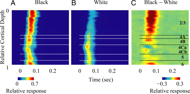
Figure 2.

Laminar pattern of population responses (MUA) to black and white stimuli. A, Color plot of responses to black stimuli in the reverse correlation experiments, as a function of recording depth in the cortex. Response here is defined as log (SNR_black) where SNR_black = σ²_black(τ)/σ²_black(−100) and where σ²_black(τ) is the spatial variance of the first order response at time offset τ. B, Color plot of responses to white stimuli in the reverse correlation experiments, as a function of recording depth in the cortex. C, Difference between black and white MUA responses as a function of depth in the cortex.

Figure 4.

Laminar pattern of relative (normalized) population responses (MUA) to black and white stimuli. A, Normalized MUA to black stimuli at different cortical depths. Normalized black responses are equal to R_black(τ)=Ar_black(τ)/max(Ar_black(τ) + Ar_white(τ)). B, Normalized MUA to white stimuli at different cortical depths where normalized white responses are R_white(τ) = Ar_white(τ)/max[Ar_black(τ) + Ar_white(τ)]. (Ar(τ) was defined as σ²(τ) − σ²(−100) for black and white, separately). Or in words, the normalized MUA to black (white) at different times is defined as the black (white) response variance at that time divided by the maximum of the sum of black and white responses during the whole response period. At each cortical depth, the MUA is estimated by the averaged activity of the recording sites within ±0.025 mm around the cortical depth. C, Black-dominant response, the difference of normalized MUA responses to black and white stimuli (black − white).

Figure 5.

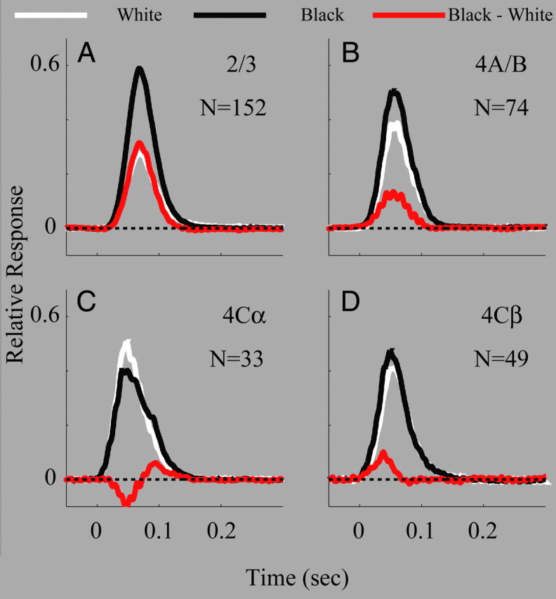
Response dynamics of population activity (MUA) to black and white stimuli in different cortical layers. A, Population-averaged time course of MUA from all recording sites in layer 2/3. B, Population-averaged time course of MUA from all recording sites in layer 4A/B. C, Population-averaged time course of MUA from all recording sites in layer 4Cα. D, Population-averaged time course of MUA from all recording sites in layer 4Cβ. In A–D, black curves represent the time courses of population activity to black stimuli; white curves represent the time courses of population activity to white stimuli; the red curves represent the difference between black and white curves. Dashed lines are zero.

Figure 6.

Time widths of population (MUA) and individual (SUA) responses to black, white, and black-dominant responses in different cortical layers. A, Time width of population responses (MUA) to black spots (black filled circles), to white spots (white filled circles) and black-dominant = black response − white response (red filled circles) in layers 2/3, 4A/B, 4Cα and 4Cβ. B, Time width of individual cell responses (SUA) to black spots (black filled circles), to white spots (white filled circles) in layers 2/3, 4A/B, 4Cα and 4Cβ. Error bars for each circle are the SD of the peak value.

Histology.

Cells were assigned to different layers of V1 based on the results of track reconstruction (Hawken et al., 1988; Ringach, 2002). Along each track, we recorded the depths of every recording site during the experiment, and then made 3–4 electrolytic lesions at 600–900 μm intervals at the end of the experiment. A lesion was made by passing a 3 μA DC current for 2 s through the quartz platinum/tungsten microelectrodes (Thomas Recording) with a stimulus generator (ALA Scientific Instruments; model STG-1001). After killing, the animal was perfused through the heart with 1 L of heparinized saline (0.01 m PBS) followed by 2–3 L of fixative (4% paraformaldehyde, 0.25% glutaraldehyde in 0.1 m phosphate buffer). After the brain was blocked and sectioned parasagittally at 50 μm, the lesions were initially located in unstained sections and then the lesion sections were stained for cytochrome oxidase. Cytochrome oxidase provides good anatomical localization of the laminar boundaries. Cortical layers were determined based on the cell density and cytochrome oxidase-specific labeling (Wong-Riley, 1979). After locating the lesions within the sections, we reconstructed the electrode penetration using a camera lucida, and determined the location of each recorded site relative to the reference lesions and the layers of the cortex. Our estimate of cortical depths of recording sites was quite precise: the difference between the estimated unit distance between lesion sites and the physical unit distance between two parallel electrodes was <5% of the average unit distance from the two measures. Therefore, factors such as the shrinkage of the brain section would not affect our estimates substantially. The mean thickness (determined for each penetration) of each layer was then used to determine each cell's normalized cortical depth ranging from 0 (representing the surface) to 1 (representing the boundary between layer 6 and the white matter). The assignment of cells to layers is crucial since the cortical connectivity of different layers in the primate cortex is very different and important for their function (Hawken et al., 1988; Lund, 1988).

Results

In this study, we used continuous signals recorded by a Thomas seven-electrode system to study the laminar pattern of population activity in response to black and white stimuli (details in Materials and Methods). Population activity was estimated by means of both MUA and the LFP. MUA and LFP are pooled responses from many single neurons. The MUA pools spike activity, a measure of suprathreshold activity, from many (on the order of 10) single neurons while it is generally agreed that the LFP is a measure of the synaptic currents, subthreshold activity, within a few hundred micrometers of the recording microelectrode (Pesaran et al., 2002; Katzner et al., 2009; Xing et al., 2009). Compared with single-unit activity, population activity significantly increased the number of neurons being studied from each recording site (Schroeder et al., 1990; Victor et al., 1994; Andersen et al., 2004; Gail et al., 2004; Pesaran et al., 2008) and enabled us to find clearer laminar patterns of black vs white dominance.

We recorded from 386 sites within V1 from five macaque monkeys. For each recording site, the spatial response map to black or white stimuli at each time delay was calculated by cross-correlation between MUA and black or white pixels in a sparse-noise stimulus. The response strength to black or white stimuli was defined as the variance of the spatial response map at each time delay (Malone et al., 2007). The signal/noise ratio, SNR, as a function of time offset τ, was defined as the ratio of the response strength to the noise, taken to be the response at −100 ms. Thus SNR_black(τ) = σ²_black(τ)/σ²_black(−100). The SNR reached a peak at a time delay between 50 and 100 ms. We chose 348/386 sites for further analysis, based on the criterion that the peak value of the SNR was >2. The numbers of recording sites are 152, 74, 33, 49, 28 and 12 sites in layer 2/3, 4A/B, 4Cα, 4Cβ, 5 and 6 respectively. Most of these recording sites were located in layers 2–4 (308/348) so in the analyses that follow we concentrate on results in the granular and supragranular layers of V1.

Laminar pattern of MUA time course to black and white stimuli

There was a clear pattern of black-dominance in the MUA time course as a function of cortical depth (Fig. 2). To visualize the depth dependence of MUA responses, we plotted the time course of the log₁₀(SNR) vs cortical depth for black (Fig. 2A) and white (Fig. 2B) responses, averaged across recording sites at each cortical depth. The average time course of log₁₀(SNR) was approximately equal for black and white in layer 4C. The average SNR for black was greater in layer 2/3 than in layer 4C (Fig. 2A) but the SNR for white was reduced in layer 2/3 compared with 4C (Fig. 2B). To make the effect clearer we plotted the difference (log₁₀(SNR _black) − log₁₀(SNR _white)) in Figure 2C. The positive values of this difference in layer 2/3 illustrate the large black-dominance in the upper layers of V1.

Visual spread of black and white responses

The sparse noise mapping technique allowed us to compare the population-average spatial summation properties for black and white stimuli across all V1 layers. As in previous work (Xing et al., 2009) we found that the spatial profiles of the spatiotemporal maps were well fit with Gaussian functions. The visual spread of MUA responses was characterized by the Gaussian SD. The visual spread for black and white was calculated separately for each recording site. The averaged visual spreads for black and white varied across cortical layers but there was not a big difference between visual spreads for black and white (Fig. 3). In particular the visual spreads were not different in the input layers 4Cα and 4Cβ. This result suggests that the mechanism for black-dominance in layer 2/3 in macaque V1 is unlikely to be a consequence of larger territories for black-sensitive inputs in the input layer, as reported for cat V1 by Jin et al. (2008). This result also suggests that the response difference between black and white stimuli is due to a difference in response amplitude not due to differences between the visual fields (visual spreads) measured by black and white stimuli.

Population-averaged time courses

To compare responses across many cortical sites that had different signal/noise ratios, we used normalized black response and normalized white response to denote the relative response strength to black stimuli or white stimuli (details in Materials and Methods). The response data were normalized by dividing the response strength (to black or white) at each time delay by the peak of the summed response strength to black and white. In this way, we were able to compare and plot the relative response strength to black and white stimuli in different cortical layers. We also defined the black-dominant response = black response − white response, as the difference between normalized black response and white response for each recording site.

The laminar dependence of the average black-dominant response of MUA was revealing (Fig. 4C). The black-dominant response was much stronger in layer 2/3 than in other layers (Fig. 4C). Also, there was a distinct black-dominant response pattern in layer 4C: a black-dominant MUA response only appeared in layer 4Cβ. In layer 4Cα, responses were white-dominant, i.e., the black-dominant response was negative there (color coded by blue).

The observations from Figure 4 were confirmed by analyzing the population-averaged black response, white response, and black-dominant response across different cortical layers (Fig. 5). The black-dominant response was strongest in layer 2/3 (its population average value was ∼0.3, significantly different from 0, p < 0.001, Fig. 5A) (see Materials and Methods for bootstrap statistics; see supplemental Fig. 1, available at www.jneurosci.org as supplemental material for individual sites). In layer 4Cβ, the black-dominant response was weak but still significantly above zero (with a population average value of ∼0.1, also significantly different from 0, p < 0.05; see supplemental Fig. 1, available at www.jneurosci.org as supplemental material for individual sites). Interestingly, the peak response in layer 4Cα was white-dominant. Thus layer 4Cα's polarity preference was different from other cortical layers including 4Cβ.

The time courses of the population-average MUA responses to black and white, and of their difference, the black-dominant response, were all important for understanding the mechanisms of black-dominance. The black-dominant response in layer 4Cβ was more transient than that in layer 2/3 (red curves in Fig. 5A,D for population averages; supplemental Fig. 2, available at www.jneurosci.org as supplemental material for individual sites). The black-dominant response persisted during the whole period of black response in layer 2/3 but it appeared mainly at the rising phase of black response in layer 4Cβ, only transiently. Analysis of both population-averaged data (Fig. 5D) and individual sites (supplemental Fig. 3, available at www.jneurosci.org as supplemental material) revealed that the transient black-dominant response in layer 4Cβ was caused by the fact that the black response was slightly faster than the white response for 4Cβ neurons.

Time widths of MUA and SUA in V1 layers

A more detailed analysis of the dynamics of neuronal responses to black and white stimuli across V1 layers was important for understanding the mechanisms of the strong black preference in layer 2/3. The quantity we analyzed was the time width of the first-order responses to black and white stimuli in the sparse noise (Fig. 6), averaged across recording sites in each layer. The time width for a black (white) response (like those illustrated in Fig. 5) was defined as the distance between the two points in time when responses were half the height of the peak response. The time widths of MUA black and white responses across V1 layers were ∼50 ms, with the one exception being the ∼60 ms time width of the white response in layer 4Cα (Fig. 6A). The black-dominant responses of MUA were of roughly comparable time widths in layers 2/3 and 4B, but were much shorter in layer 4C, indicating the very transient black-dominant responses in the input layers (Fig. 6A). SUA to black and white had time widths that were 40–45 ms in all layers (Fig. 6B), similar to, though slightly smaller than, those of MUA. Comparison of the time widths in Figure 5 with predictions of circuit models was the next step in the analysis.

Is the black-dominance in layer 2/3 due to the black-dominant responses in layer 4Cβ?

A general scheme for the amplification of input differences (here the difference is black vs white response) is through a nonselective mechanism, such as by a threshold, by a static nonlinearity, or by a constant inhibition, which can remove the same amount of response from two different responses and therefore enlarge the relative difference between two different signals. In such a model, a system does not care about the input type, but only cares about the input amplitude.

One nonselective model we considered was the following: the black-dominant response (Fig. 4C) in layer 2/3 was generated by a sum of the responses of layer 4Cβ neurons and then the summed response had to exceed a high threshold to evoke responses in layer 2/3 (Fig. 7A). While a high threshold can enlarge the difference of black and white responses by removing the big baseline of balanced black and white responses from layer 4Cβ, the time widths of both black and white responses in layer 2/3 should be much smaller than those of the black (white) responses in layer 4Cβ (Fig. 7A). This prediction from a nonselective scheme is not consistent with our physiological observations that black and white responses were roughly constant in time width across all layers studied, including layers 4Cβ and 2/3 (see the black points representing time widths of black responses in Fig. 6; also compare Fig. 5).

Figure 7.

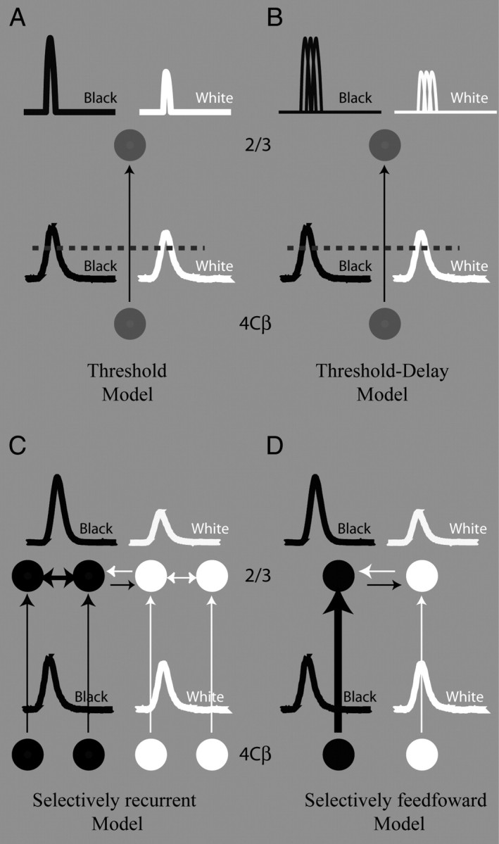
Schematic models for black-dominant responses in layer 2/3. A, Nonselective threshold model for information transferred from layer 4Cβ to layer 2/3. Black and white curves on the bottom of A represent population responses to black and white stimuli in layer 4Cβ. Black and white curves at the top of A represent population responses to black and white stimuli in layer 2/3 after thresholding (marked by a horizontal dashed line). Notice that the response in the model's layer 2/3 is much more transient than that in layer 4Cβ. B, More complicated nonselective threshold model for information transferred from layer 4Cβ to layer 2/3. Black and white curves at the bottom of B represent population responses to black and white stimuli in layer 4Cβ. Black and white curves at the top of B represent population responses to black and white stimuli in layer 2/3 after thresholding (marked by a horizontal dashed line). Notice that the response in the model's layer 2/3 is much more transient than that in layer 4Cβ. C, Recurrent model with a selective amplification of black responses for information transferred from layer 4Cβ to layer 2/3. Black and white curves at the bottom of C represent population responses to black and white stimuli in layer 4Cβ. Black and white curves on the top of C represent population responses to black and white stimuli in layer 2/3. D, Feedforward model with a selective amplification of black responses for information transferred from layer 4Cβ to layer 2/3. Black and white curves at the bottom of D represent population responses to black and white stimuli in layer 4Cβ. Black and white curves at the top of D represent population responses to black and white stimuli in layer 2/3.

Furthermore, a nonselective model also predicts that if the time width of the black response is larger than that of the black-dominant response in layer 4Cβ it should also be larger in layer 2/3. The experimental results also do not agree with this prediction from a nonselective model (Fig. 6A for MUA population results; supplemental Fig. 2, available at www.jneurosci.org as supplemental material for individual sites). In 4Cβ, the black-dominant response was much more transient than the response to black alone. But in layer 2/3 the black-dominant MUA response and the response to black itself had roughly the same time width.

We further ruled out a more complicated nonselective model in which MUA activity in layer 2/3 reflects the summed spike activity of many single cells in layer 2/3 each of which has a high threshold and therefore has a narrower response time course than its input, as in Figure 7B. In fact, the time width of single-cell responses in layer 2/3 was roughly the same as that of MUA in layer 2/3. Therefore, based on considerations of response timing, we conclude that the underlying mechanism for black-dominant responses in layer 2/3 has to be more complicated than a model comprised of feedforward input followed by a nonselective nonlinearity.

Another observation that argues against nonselective models is that the MUA response in layer 5 was almost equal for black and white stimuli (Figs. 2–4). A nonselective enhancement by thresholding of the small imbalance of black and white responses present in layer 4Cβ would have caused a larger black response in layer 5 neurons that should have been evident in MUA in layer 5. This prediction was not observed.

Selective models

Another class of models that are possible explanations for the cortical generation of black-dominance in layer 2/3 is illustrated in Figure 7, C and D. In this type of model, the system cares about input types (here the different types are black vs white response) and it treats inputs differently based on the type of input. Therefore we can call it a selective model. One such selective model is selective recurrent excitation between black-dominant cells within layer 2/3 (Fig. 7C). Another is selectively greater connectivity from cells in layer 4Cβ with larger black-dominant responses to cells in layer 2/3 (Fig. 7D). The selective-recurrent and selective-connectivity models are not mutually exclusive.

Dynamics of the LFP and MUA in response to black and white stimuli

We further calculated the dynamic response of the LFP to test the input-output relationship proposed in the selective models. The LFP, which measures the subthreshold activity in a local cortical region, serves as a complementary signal to the MUA. Similar to the laminar pattern of MUA, we plotted the LFP responses to black and white stimuli (Fig. 8A,B) and the black-dominant LFP response as a function of cortical depth (Fig. 8C). The LFP showed a similar laminar-specific pattern of black, white and black-dominant responses as the MUA, though there were some quantitative differences between the two signals (Figs. 4, 8). The black-dominant response of the LFP in layer 2/3 was stronger than in any other layers (Fig. 8). Unlike MUA, the LFP responses to black or white had two peaks in time (Fig. 8A,B); both peaks had a black-dominant response (Fig. 8C). In this study we only focused on the first early LFP peak that overlapped with MUA in time.

Figure 8.

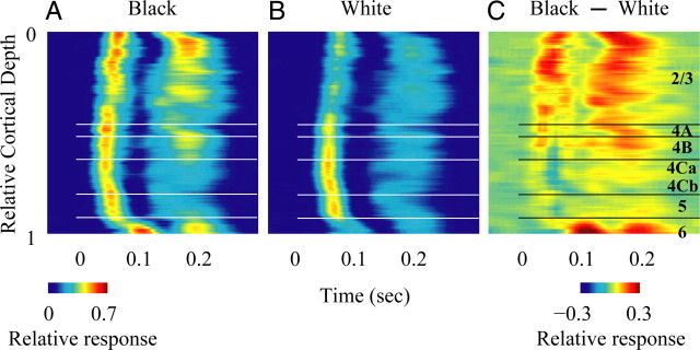
Laminar pattern of population responses (LFP) to black and white stimuli. A, The local field potential (LFP) to black stimuli at different cortical depth. B, The LFP to white stimuli at different cortical depth. For each recording site, the LFP to black (white) at different time points is represented by black (white) response variance at that time divided by the maximum variance of the sum of black and white response variance during the whole response period. At each cortical depth, the LFP is estimated by the averaged activity of the recording sites within ±50 μm around the cortical depth. C, Difference of the LFP to black and white stimuli.

Comparisons of LFP and MUA black-dominant responses

The time course of the black-dominant response of the LFP (Fig. 9, blue curve) was not identical to the time course of MUA either in layer 4Cβ (Fig. 9, green curve) or in layer 2/3 (Fig. 9, red curve). On the rising phase, the LFP time course in layer 2/3 tracked the time course of MUA in layer 4Cβ, which is consistent with the idea that the early component of the LFP in layer 2/3 was related to the synaptic current driven by spikes from the input to layer 2/3, namely spikes from layer 4Cβ. However, the black-dominant response in the LFP in layer 2/3 was much more sustained than that of the MUA in layer 4Cβ (Fig. 9). At a time when the black-dominant component of MUA in layer 4Cβ decayed back to 0, the layer 2/3 LFP was still producing a black-dominant response. This suggests that the black-dominant response could have been initiated by input from layer 4Cβ neurons, and that recurrent local circuitry in layer 2/3 also could have played a role in amplifying and prolonging the black-dominant response of layer 2/3. Furthermore, the fact that the black-dominant response of the LFP was more prolonged in layer 2/3 compared with its input from layer 4Cβ MUA implies that the LFP did not reflect only its feedforward input but also local circuit activity.

Figure 9.

A comparison of response dynamics for the LFP and MUA in layer 2/3 and layer 4Cβ. The red curve represents the time course of the difference between black and white MUA responses in layer 2/3. The blue curve represents the time course of the difference between black and white LFP responses in layer 2/3. The green curve represents the time course of the difference between black and white MUA responses in layer 4Cβ.

Discussion

In this study, we studied the laminar pattern of population activity by means of both MUA and the LFP in response to black and white stimuli. The population activity enabled us to measure a clear laminar pattern efficiently. In different layers, a small preference for black appeared in early responses in layer 4Cβ, the parvocellular-input layer, but not in the magnocellular-input layer 4Cα. However, further analysis of the dynamics of black-white responses in different layers suggested that a small preference for black in layer 4Cβ was not the main reason for black-dominant responses in layer 2/3. Rather, the data required selective connectivity and amplification of signals about black stimuli. We hypothesize that black-selective wiring could be due to (1) selective feedforward connections from black-dominant neurons in layer 4C to cells in layer 2/3 or (2) selective recurrent interactions between black-dominant neurons in layer 2/3, or a combination of both (1) and (2).

Neuronal mechanisms for generating black-dominant responses in cortex

Because of the dynamic differences of black-dominant responses in layer 4Cβ and layer 2/3 and the constant time width for black responses in all layers, we ruled out a simple feedforward-plus-threshold mechanism that amplifies response differences nonselectively in layer 2/3. Furthermore, the near equality of time width between single-unit and multiunit visually evoked responses in layer 2/3 also ruled out a more elaborate nonselective model that includes dispersion of the time-to-peak of narrower single-unit responses. Instead we need to consider different mechanisms, either 1) a selective-recurrent excitatory-inhibitory network in layer 2/3, for amplifying the black-dominant signal from layer 4Cβ to layer 2/3 and suppressing responses to white, or 2) selective connectivity of black-dominant neurons in layer 4Cβ to layer 2/3, or both 1) and 2).

Selective recurrent models

Recurrent models have been proposed earlier for amplifying cortical responses to preferred stimuli (Ben-Yishai et al., 1995; Douglas et al., 1995). Recurrent networks may be a general mechanism of amplification for many neuronal functional properties in the brain (Douglas and Martin, 2007), such as orientation selectivity (Ringach et al., 2003; Xing et al., 2004), direction selectivity (Reid et al., 1987; Hawken et al., 1988), as well as black-dominant responses in visual cortex. Recurrent network interactions have been suggested to be the neural substrate for sound frequency selectivity in auditory cortex (Wehr and Zador, 2003; Zhang et al., 2003) and direction selectivity in somatosensory cortex (Wilent and Contreras, 2005). The SNR data (see Figs. 2, 4, 5, 6) suggest that both recurrent excitation and inhibition in layer 2/3 could play a role in respectively enhancing black responses and suppressing white responses in layer 2/3.

Selective feedforward connectivity

Another hypothesis that the data do not rule out is selective wiring of black-preferring neurons in layer 4C to layer 2/3 neurons. Our previous single-unit study (Yeh et al., 2009a) reported that there were both black- and white-preferring neurons in layer 4C, consistent with the results reported here for MUA in layer 4C. If during development the black-preferring 4C neurons made more excitatory connections with target neurons in layer 2/3, that could be part of the explanation for the great amplification of black dominance in layer 2/3. The LFP data in Figures 8 and 9 are relevant here. The average black-dominance of the rising phase of the layer 2/3 LFP was not larger than that seen in MUA in layer 4Cβ. However, the LFP black-dominance could have been diluted by inputs to layer 2/3 from other sources not from layer 4C, so the quantitative comparison is not decisive. A model with selective feedforward connections thus remains an open possibility.

Jin et al. (2008) have provided a selective mechanism for black-dominance in layer 4 of cat V1 (area 17). They found that the termination zones of off-center LGN afferents were wider than those of on-center afferents in terms of cortical territory. However, we think Jin et al.'s finding in cat does not providea mechanism for the large black-dominance we observed in layer 2/3 of macaque, because 1) as reported in this paper and also in Yeh et al. (2009a), there were roughly balanced responses to black and white in the input layer 4C in macaque V1; 2) there was not a big difference between visual spreads for black and white in macaque V1 (Fig. 3). In particular the visual spreads were not different in the input layers 4Cα and 4Cβ. These results suggest that the mechanism for black-dominance in layer 2/3 in macaque V1 is not due to larger territories for black-sensitive inputs in the input layer.

Is extrastriate feedback involved in setting up a preference for black in V1?

Another explanation for the emergence of black-dominant responses in layer 2/3 could be feedback from extrastriate cortex to V1. If feedback enhances the black response, one would expect that the spatial spread of the black response would be larger because the feedback from extrastriate neurons is more extensive in visual space than the visual receptive fields of V1 neurons (Angelucci et al., 2002). The idea of feedback was testable with our dataset because we measured visual spreads for black and white stimuli (Fig. 3). The data do not support the proposal for enhancement by feedback because there is little expansion of visual spatial summation in black and white responses in layer 2/3 (Fig. 3). It is likely that the sparse-noise stimulus used to drive visual responses in V1 in our experiments was an ineffective stimulus for the large receptive fields of neurons in extrastriate cortex, and this is why feedback appears not to have influenced the V1 responses we measured. As previously reported, the degree of black-dominance measured was strongly affected by the stimulus ensemble (Yeh et al., 2009a,b).

Methodology: laminar analysis of multiunit activity and the local field potential

In this study, we analyzed MUA and the LFP from continuous neuronal signals recorded by a Thomas multielectrode system. Also, we combined the population analysis with laminar reconstruction of recording sites. Using population responses to study the laminar variation of functional properties (Figs. 2–6, 8, 9) has big advantages relative to traditional methods that use single-unit activity. Population activity increases the number of neurons that can be studied at each cortical depth. Measurement of population activity may blur some response properties of single neurons in layer 4Cβ, but it provides a much faster and more reliable way to describe the global picture of the transfer of neuronal information between different layers (Mitzdorf, 1987; Schroeder et al., 1990; Victor et al., 1994). Our results for both MUA and the LFP have shown a clear laminar variation of the black-dominant response. This laminar variation not only validates our methods of track reconstruction, but also suggests that MUA and the LFP are signals from a very local region not only within the same cortical layers horizontally but also across different layers vertically (Xing et al., 2009). While population activity recorded electrophysiologically as in our experiments is not as precise spatially as single-unit activity, it has a spatial resolution much finer than other population measures, such as intrinsic optical imaging, fMRI, MEG, and EEG. Measuring population activity with multielectrode recording in different cortical areas provides an important tool for studying neural networks in the brain that is complementary to both single-unit recording and functional imaging methods.

References

- Andersen RA, Burdick JW, Musallam S, Scherberger H, Pesaran B, Meeker D, Corneil BD, Fineman I, Nenadic Z, Branchaud E, Cham JG, Greger B, Tai YC, Mojarradi MM. Recording advances for neural prosthetics. Conf Proc IEEE Eng Med Biol Soc. 2004;7:5352–5355. doi: 10.1109/IEMBS.2004.1404494. [DOI] [PubMed] [Google Scholar]
- Angelucci A, Levitt JB, Lund JS. Anatomical origins of the classical receptive field and modulatory surround field of single neurons in macaque visual cortical area V1. Prog Brain Res. 2002;136:373–388. doi: 10.1016/s0079-6123(02)36031-x. [DOI] [PubMed] [Google Scholar]
- Benardete EA, Kaplan E. The receptive field of the primate P retinal ganglion cell, I: linear dynamics. Vis Neurosci. 1997;14:169–185. doi: 10.1017/s0952523800008853. [DOI] [PubMed] [Google Scholar]
- Benardete EA, Kaplan E. Dynamics of primate P retinal ganglion cells: responses to chromatic and achromatic stimuli. J Physiol. 1999;519:775–790. doi: 10.1111/j.1469-7793.1999.0775n.x. [DOI] [PMC free article] [PubMed] [Google Scholar]
- Ben-Yishai R, Bar-Or RL, Sompolinsky H. Theory of orientation tuning in visual cortex. Proc Natl Acad Sci U S A. 1995;92:3844–3848. doi: 10.1073/pnas.92.9.3844. [DOI] [PMC free article] [PubMed] [Google Scholar]
- Blackwell HR. Contrast thresholds of the human eye. J Opt Soc Am. 1946;36:624–643. doi: 10.1364/josa.36.000624. [DOI] [PubMed] [Google Scholar]
- Bowen RW, Pokorny J, Smith VC. Sawtooth contrast sensitivity: decrements have the edge. Vision Res. 1989;29:1501–1509. doi: 10.1016/0042-6989(89)90134-x. [DOI] [PubMed] [Google Scholar]
- Chichilnisky EJ, Kalmar RS. Functional asymmetries in ON and OFF ganglion cells of primate retina. J Neurosci. 2002;22:2737–2747. doi: 10.1523/JNEUROSCI.22-07-02737.2002. [DOI] [PMC free article] [PubMed] [Google Scholar]
- Chubb C, Nam JH. Variance of high contrast textures is sensed using negative half-wave rectification. Vision Res. 2000;40:1677–1694. doi: 10.1016/s0042-6989(00)00007-9. [DOI] [PubMed] [Google Scholar]
- Chubb C, Landy MS, Econopouly J. A visual mechanism tuned to black. Vision Res. 2004;44:3223–3232. doi: 10.1016/j.visres.2004.07.019. [DOI] [PubMed] [Google Scholar]
- Dannemiller JL, Stephens BR. Asymmetries in contrast polarity processing in young human infants. J Vis. 2001;1:112–125. doi: 10.1167/1.2.5. [DOI] [PubMed] [Google Scholar]
- Douglas RJ, Martin KA. Recurrent neuronal circuits in the neocortex. Curr Biol. 2007;17:R496–R500. doi: 10.1016/j.cub.2007.04.024. [DOI] [PubMed] [Google Scholar]
- Douglas RJ, Koch C, Mahowald M, Martin KA, Suarez HH. Recurrent excitation in neocortical circuits. Science. 1995;269:981–985. doi: 10.1126/science.7638624. [DOI] [PubMed] [Google Scholar]
- Gail A, Brinksmeyer HJ, Eckhorn R. Contour decouples gamma activity across texture representation in monkey striate cortex. Cereb Cortex. 2000;10:840–850. doi: 10.1093/cercor/10.9.840. [DOI] [PubMed] [Google Scholar]
- Gail A, Brinksmeyer HJ, Eckhorn R. Perception-related modulations of local field potential power and coherence in primary visual cortex of awake monkey during binocular rivalry. Cereb Cortex. 2004;14:300–313. doi: 10.1093/cercor/bhg129. [DOI] [PubMed] [Google Scholar]
- Hawken MJ, Parker AJ, Lund JS. Laminar organization and contrast sensitivity of direction-selective cells in the striate cortex of the Old World monkey. J Neurosci. 1988;8:3541–3548. doi: 10.1523/JNEUROSCI.08-10-03541.1988. [DOI] [PMC free article] [PubMed] [Google Scholar]
- Jin JZ, Weng C, Yeh CI, Gordon JA, Ruthazer ES, Stryker MP, Swadlow HA, Alonso JM. On and off domains of geniculate afferents in cat primary visual cortex. Nat Neurosci. 2008;11:88–94. doi: 10.1038/nn2029. [DOI] [PMC free article] [PubMed] [Google Scholar]
- Jones JP, Palmer LA. The two-dimensional spatial structure of simple receptive fields in cat striate cortex. J Neurophysiol. 1987;58:1187–1211. doi: 10.1152/jn.1987.58.6.1187. [DOI] [PubMed] [Google Scholar]
- Katzner S, Nauhaus I, Benucci A, Bonin V, Ringach DL, Carandini M. Local origin of field potentials in visual cortex. Neuron. 2009;61:35–41. doi: 10.1016/j.neuron.2008.11.016. [DOI] [PMC free article] [PubMed] [Google Scholar]
- Kontsevich LL, Tyler CW. Nonlinearities of near-threshold contrast transduction. Vision Res. 1999;39:1869–1880. doi: 10.1016/s0042-6989(98)00286-7. [DOI] [PubMed] [Google Scholar]
- Krauskopf J. Discrimination and detection of changes in luminance. Vision Res. 1980;20:671–677. doi: 10.1016/0042-6989(80)90091-7. [DOI] [PubMed] [Google Scholar]
- Kremers J, Lee BB, Pokorny J, Smith VC. Responses of macaque ganglion cells and human observers to compound periodic waveforms. Vision Res. 1993;33:1997–2011. doi: 10.1016/0042-6989(93)90023-p. [DOI] [PubMed] [Google Scholar]
- Krüger J, Fischer B. Symmetry between the visual B- and D-systems and equivalence of center and surround: studies of light increment and decrement in retinal and geniculate neurons of the cat. Biol Cybern. 1975;20:223–236. doi: 10.1007/BF00342642. [DOI] [PubMed] [Google Scholar]
- Lankheet MJ, Lennie P, Krauskopf J. Distinctive characteristics of subclasses of red-green P-cells in LGN of macaque. Vis Neurosci. 1998;15:37–46. doi: 10.1017/s0952523898151027. [DOI] [PubMed] [Google Scholar]
- Lund JS. Anatomical organization of macaque monkey striate visual cortex. Annu Rev Neurosci. 1988;11:253–288. doi: 10.1146/annurev.ne.11.030188.001345. [DOI] [PubMed] [Google Scholar]
- Malone BJ, Kumar VR, Ringach DL. Dynamics of receptive field size in primary visual cortex. J Neurophysiol. 2007;97:407–414. doi: 10.1152/jn.00830.2006. [DOI] [PubMed] [Google Scholar]
- Mitzdorf U. Properties of the evoked potential generators: current source-density analysis of visually evoked potentials in the cat cortex. Int J Neurosci. 1987;33:33–59. doi: 10.3109/00207458708985928. [DOI] [PubMed] [Google Scholar]
- Olman C, Boyaci H, Fang F, Doerschner K. V1 responses to different types of luminance histogram contrast. [Visual Science Society Abstract.] J Vis. 2008;8:345a. [Google Scholar]
- Pesaran B, Pezaris JS, Sahani M, Mitra PP, Andersen RA. Temporal structure in neuronal activity during working memory in macaque parietal cortex. Nat Neurosci. 2002;5:805–811. doi: 10.1038/nn890. [DOI] [PubMed] [Google Scholar]
- Pesaran B, Nelson MJ, Andersen RA. Free choice activates a decision circuit between frontal and parietal cortex. Nature. 2008;453:406–409. doi: 10.1038/nature06849. [DOI] [PMC free article] [PubMed] [Google Scholar]
- Reid RC, Soodak RE, Shapley RM. Linear mechanisms of directional selectivity in simple cells of cat striate cortex. Proc Natl Acad Sci U S A. 1987;84:8740–8744. doi: 10.1073/pnas.84.23.8740. [DOI] [PMC free article] [PubMed] [Google Scholar]
- Ringach DL. Spatial structure and symmetry of simple-cell receptive fields in macaque primary visual cortex. J Neurophysiol. 2002;88:455–463. doi: 10.1152/jn.2002.88.1.455. [DOI] [PubMed] [Google Scholar]
- Ringach DL, Hawken MJ, Shapley R. Dynamics of orientation tuning in macaque V1: the role of global and tuned suppression. J Neurophysiol. 2003;90:342–352. doi: 10.1152/jn.01018.2002. [DOI] [PubMed] [Google Scholar]
- Schroeder CE, Tenke CE, Givre SJ, Arezzo JC, Vaughan HG., Jr Laminar analysis of bicuculline-induced epileptiform activity in area 17 of the awake macaque. Brain Res. 1990;515:326–330. doi: 10.1016/0006-8993(90)90617-k. [DOI] [PubMed] [Google Scholar]
- Short AD. Decremental and incremental visual thresholds. J Physiol. 1966;185:646–654. doi: 10.1113/jphysiol.1966.sp008007. [DOI] [PMC free article] [PubMed] [Google Scholar]
- Tyler CW, Chan H. Increment and decrement asymmetries: implications for pattern detection and appearance. Proc Soc Inform Display. 1992;23:251–254. [Google Scholar]
- Victor JD, Purpura K, Katz E, Mao B. Population encoding of spatial frequency, orientation, and color in macaque V1. J Neurophysiol. 1994;72:2151–2166. doi: 10.1152/jn.1994.72.5.2151. [DOI] [PubMed] [Google Scholar]
- Wehr M, Zador AM. Balanced inhibition underlies tuning and sharpens spike timing in auditory cortex. Nature. 2003;426:442–446. doi: 10.1038/nature02116. [DOI] [PubMed] [Google Scholar]
- Whittle P. Increments and decrements: luminance discrimination. Vision Res. 1986;26:1677–1691. doi: 10.1016/0042-6989(86)90055-6. [DOI] [PubMed] [Google Scholar]
- Wilent WB, Contreras D. Dynamics of excitation and inhibition underlying stimulus selectivity in rat somatosensory cortex. Nat Neurosci. 2005;8:1364–1370. doi: 10.1038/nn1545. [DOI] [PubMed] [Google Scholar]
- Wong-Riley M. Changes in the visual system of monocularly sutured or enucleated cats demonstrable with cytochrome oxidase histochemistry. Brain Res. 1979;171:11–28. doi: 10.1016/0006-8993(79)90728-5. [DOI] [PubMed] [Google Scholar]
- Xing D, Ringach DL, Shapley R, Hawken MJ. Correlation of local and global orientation and spatial frequency tuning in macaque V1. J Physiol. 2004;557:923–933. doi: 10.1113/jphysiol.2004.062026. [DOI] [PMC free article] [PubMed] [Google Scholar]
- Xing D, Yeh CI, Shapley RM. Spatial spread of the local field potential and its laminar variation in visual cortex. J Neurosci. 2009;29:11540–11549. doi: 10.1523/JNEUROSCI.2573-09.2009. [DOI] [PMC free article] [PubMed] [Google Scholar]
- Yeh CI, Xing D, Shapley RM. “Black” responses dominate macaque primary visual cortex v1. J Neurosci. 2009a;29:11753–11760. doi: 10.1523/JNEUROSCI.1991-09.2009. [DOI] [PMC free article] [PubMed] [Google Scholar]
- Yeh CI, Xing D, Williams PE, Shapley RM. Stimulus ensemble and cortical layer determine V1 spatial receptive fields. Proc Natl Acad Sci U S A. 2009b;106:14652–14657. doi: 10.1073/pnas.0907406106. [DOI] [PMC free article] [PubMed] [Google Scholar]
- Zemon V, Gordon J, Welch J. Asymmetries in ON and OFF visual pathways of humans revealed using contrast-evoked cortical potentials. Vis Neurosci. 1988;1:145–150. doi: 10.1017/s0952523800001085. [DOI] [PubMed] [Google Scholar]
- Zemon V, Eisner W, Gordon J, Grose-Fifer J, Tenedios F, Shoup H. Contrast-dependent responses in the human visual system: childhood through adulthood. Int J Neurosci. 1995;80:181–201. doi: 10.3109/00207459508986100. [DOI] [PubMed] [Google Scholar]
- Zhang LI, Tan AY, Schreiner CE, Merzenich MM. Topography and synaptic shaping of direction selectivity in primary auditory cortex. Nature. 2003;424:201–205. doi: 10.1038/nature01796. [DOI] [PubMed] [Google Scholar]