Hierarchical Adaptive Regression Kernels for Regression with Functional Predictors

Abstract

We propose a new method for regression using a parsimonious and scientifically interpretable representation of functional predictors. Our approach is designed for data that exhibit features such as spikes, dips, and plateaus whose frequency, location, size, and shape varies stochastically across subjects. We propose Bayesian inference of the joint functional and exposure models, and give a method for efficient computation. We contrast our approach with existing state-of-the-art methods for regression with functional predictors, and show that our method is more effective and efficient for data that include features occurring at varying locations. We apply our methodology to a large and complex dataset from the Sleep Heart Health Study, to quantify the association between sleep characteristics and health outcomes. Software and technical appendices are provided in online supplemental materials.

1. INTRODUCTION

Due to technological advancements an increasing number of studies involve functional data such as images or time series. The Sleep Heart Health Study (Quan et al. 1997; Di, Crainiceanu, Caffo, and Punjabi 2009) relates sleep patterns, as measured using electroencephalogram (EEG) data, to health outcomes, such as cardiovascular health indicators. As in this example, the functional datum is often the predictor in a regression problem. Other examples include estimating chemical variables from spectroscopic data (Osbourne, Fearn, Miller and Douglas 1984), predicting annual precipitation from daily temperature data (Ramsay and Silverman 2005), and relating magnetic resonance imaging data or diffusion tensor imaging data to health outcomes (Goldsmith, Bobb, Crainiceanu, Caffo and Reich 2011).

We introduce a new approach to regression with functional predictors, based on a kernel mixture functional representation. This representation is designed for predictors that exhibit features such as dips, bumps, and plateaus whose frequency, location, size, and shape varies stochastically across subjects. We use this representation of the functional covariates for predicting a scalar outcome. Summaries of the representation, such as the frequency of bumps, or average height or width of the bumps, can have intuitive scientific interpretation; we regress the outcome on these functional summaries. This approach does not require alignment or even a common domain for the subject-specific functions. It also does not require the function observation locations to be equally spaced, and naturally handles missing or co-located data. Mathematically, nearly all existing methods for regression with a functional predictor represent the predictor using a set of linearly independent basis functions; we instead represent the predictor using an uncountable and linearly dependent dictionary of generating elements. Regularization is induced through the prior distribution, and consistency properties still hold. This more flexible representation allows for the above scientific interpretation of events occurring at random locations, and the ability to relate those events to the outcome variable.

Our methodology is motivated by data from the Sleep Heart Health Study, and by interest in using these data to understand the relationship between sleep characteristics and health outcomes. Some of the challenges associated with these data are the large numbers of patients, large number of observations per patient, missing data, and complex variability patterns. Most importantly, the sleep EEG data are desynchronized across patients; each patient goes through sleep cycles whose length, number, and features vary across subjects and may be related to the health outcomes. This desynchronization is clearly visible in Figure 1, which shows the EEG signals of four subjects. Standard functional regression approaches incorrectly treat the time series as being aligned; registration of the signals (Ramsay and Silverman 2005) to achieve alignment is inappropriate since the number and features of the sleep cycles vary widely across subjects. By contrast, our predictor representation naturally captures the presence of sleep cycles occurring at random times.

Figure 1.

EEG (δ power) series for four subjects, with penalized spline approximations.

In order to fully account for uncertainty in the functions when obtaining inferences for the regression coefficients, we introduce a joint hierarchical model. Failure to account for this uncertainty can lead to biased estimation and incorrect standard errors (Carroll, Ruppert, Stefanski and Crainiceanu 2006; Crainiceanu, Staicu and Di 2009). We call our approach Hierarchical Adaptive Regression Kernels (HARK). We show that this method is computationally feasible using an approximation to the posterior distribution obtained via a technique called “modularization” or “cutting feedback” (Liu, Bayarri and Berger 2009; Lunn, Best, Spiegelhalter, Graham and Neuenschwander 2009; McCandless, Douglas, Evans and Smeeth 2010). With this approximation the slower part of the computation can be done in parallel across subjects, so even a very large number of subjects can be handled easily. In the process we correct a problem in the modularization method as used in the above citations: while the modularization approximation yields a well-defined joint distribution on the parameters, the Markov chain methods previously used were not guaranteed to converge to that distribution.

The functional representation we utilize has been used previously for consistent nonparametric estimation of a single function under the name Lévy Adaptive Regression Kernels (LARK: Clyde, House, and Wolpert 2006; Wolpert, Clyde, and Tu 2006). Our approach is different from LARK because we: (1) model a population of functions, where the frequency, location, and shape of the features vary across subjects; (2) predict an outcome on that population; (3) introduce a method for efficient posterior computation for the joint functional and exposure models, over the entire population.

We contrast our approach with a state-of-the-art method for regression with a functional predictor, Penalized Functional Regression (PFR: Goldsmith, Bobb, Crainiceanu, Caffo, and Reich 2011; Crainiceanu and Reiss 2011). Like some other existing methods (Cardot, Ferraty and Sarda 2003; Reiss and Ogden 2007), PFR assumes that the functional predictor has a common domain across subjects (perhaps after registration), and that the outcome is linearly related to the function value f_i(x) at each location x. The latter implicitly assumes alignment of the predictor across subjects.

We show that for simulated data that include features that occur at random locations, PFR requires a large amount of data to detect any relationship between the predictor and the outcome, and is unable to represent that relationship accurately for any sample size. By contrast, HARK can capture the relationship effectively even for small sample sizes (see Section 5). Conversely, if the data are generated from the functional linear model (defined in Section 2) PFR works well and HARK does not effectively capture the relationship between predictor and outcome. Applying both HARK and PFR to the sleep data, HARK detects several important relationships that PFR does not, for instance that the frequency and magnitude of fluctuations in the EEG series are negatively associated with the respiratory disturbance index of the subject.

Alternative methods for joint modeling of a functional predictor and scalar outcome are given in Bigelow and Dunson (2009) and Dunson (2010). These approaches represent the subject-specific functions f_i(x) using a basis expansion and estimate the distribution of the resulting coefficient vectors, either jointly with the outcome or conditional on the outcome. Since these methods relate the outcome to the coefficients of a basis expansion, they still assume alignment of the subject-specific functions. In relating the coefficients to the outcome these methods are extremely flexible. Since they must estimate a distribution with dimension greater than or equal to the number of bases, for statistical efficiency reasons they either use a small number of bases (the choice of which can be learned from the data; Bigelow and Dunson 2009) or make substantial assumptions about the structure of this distribution (Dunson 2010).

Section 2 introduces our model for the subject-specific functions, and Section 3 links the subject-level models hierarchically to a regression model; Section 4 describes our computational procedure. Section 5 gives a simulation study, and HARK and PFR are applied to the sleep data in Section 6.

2. FUNCTIONAL DATA MODEL

First we describe the nonparametric functional representation we use. For each subject i we have noisy observations ${\left\{W_i\right(x_{ik}\left)\right\}}_{k=1}^{K_i}$ of a functional predictor fi(x) at locations x_ik in the (potentially subject-specific) domain ${\mathcal{X}}_i$. To represent the functional predictor we utilize the mixture form

$$f_i\left(x\right)={\beta }_{0i}\left(x\right)+\sum _{m=1}^{M_i}{\gamma }_{im}\mathcal{K}(x,s_{im}).$$ (1)

Here $\mathcal{K}(x,s)$ is a specified kernel function on ${\mathcal{X}}_i\times \mathcal{S}$, where the parameters of the kernel are defined on a space $\mathcal{S}$. Also, M_i < ∞ is the number of mixture components, and γ_im ∈ ℝ and $s_{im}\in \mathcal{S}$ are the magnitudes and parameter vectors of those mixture components, respectively. All of these quantities except the kernel function $\mathcal{K}$ are taken to be unknown. The scaling and other parameters are allowed to vary between the components, “adapting” to the local features of the function. The background signal β_0i(x) typically has a parametric form, such as a polynomial function of x; for simplicity we take β_0i(x) = β_0i to be an unknown constant but extensions to more general forms are straightforward (cf. Best, Ickstadt, and Wolpert 2000).

Contrast this with standard functional data analysis approaches, which do not model the functional predictor directly; instead, they typically assume that the outcome is linearly related to ∫f_i(x)β(x)dx for some function β(x). This framework is called the functional linear model with scalar response (Cardot et al. 2003; Müller and Stadtm̈uller 2005). It is implemented by representing the functional predictor as a weighted sum of linearly independent basis functions, and using the coefficients from this representation as predictors in a standard regression model. Examples of bases include principal component functions (cf. Müller and Stadtmüller 2005; Goldsmith et al. 2011), spline bases (cf. James 2002), the Fourier basis (cf. Ramsay and Silverman 2005), or partial least squares factors (cf. Goutis and Fearn 1996; Reiss and Ogden 2007). Estimation in the regression model proceeds via traditional methods (e.g. least squares) or by incorporating a roughness penalty (Marx and Eilers 1999; Cardot et al. 2003).

The kernel mixture (1) can also be viewed as representing f_i(·) via a linear expansion, but instead of linearly independent basis functions an uncountable and linearly dependent dictionary of generating elements is used. Although the coefficients are no longer unique, one can obtain a more parsimonious representation, by using fewer non-zero coefficients to attain the same accuracy. Regularization is induced through the prior distribution; this effect is described in detail in Clyde and Wolpert (2007). Sufficient conditions for consistency of function estimation using such kernel mixture models are given in Pillai (2008).

The kernel mixture representation (1) has been used previously for Bayesian estimation of a single function by applying a Lévy process prior for the mixture components; this approach is called Lévy Adaptive Regression Kernels (LARK: Clyde, House, and Wolpert 2006; Wolpert, Clyde, and Tu 2011). LARK models have been applied to one-dimensional curve fitting and spatial and spatio-temporal modeling in Wolpert, Clyde and Tu (2011) and Woodard, Wolpert and O’Connell (2010). They have also been used for peak identification in mass spectroscopy (House 2006; Clyde, House and Wolpert 2006; House, Clyde and Wolpert 2010).

Instead of estimating a single function as in these citations, we estimate a population of functions where the number, magnitude, and parameters of the mixture components vary across the population; furthermore, we use the functions to predict outcomes. Our approach is distinct, for instance, from the approach of MacLehose and Dunson (2009), which represents the functions using the kernel mixture form (1) but takes a common set of mixture components across subjects. It is also different from the hierarchical model of House (2006), which uses (1) but takes a common M_i = M and specifies ${\left\{\right({\gamma }_{im},s_{im}\left)\right\}}_{m=1}^{M_i}$ as random effects centered at a common set of components ${\left\{\right({\gamma }_m,s_m\left)\right\}}_{m=1}^{M_i}$.

The most natural way to model a population of functions is via a hierarchical specification, allowing borrowing of information across the population (Bigelow and Dunson 2007; MacLehose and Dunson 2009). However, this approach is very computationally intensive when the number of subjects is large, since all functions must be simultaneously estimated. To facilitate computation we will assign independent prior distributions to the subject-specific functional representations. However, in the spirit of hierarchical modeling we estimate the hyperparameters of those prior distributions from the population of functions in an empirical Bayes fashion. This approach can be viewed as an empirical version of hierarchical modeling of the population of functions, that scales more effectively to large and complex applications like the sleep study.

We do not use a Lévy process prior for the functional representations. The prior we use is more flexible and facilitates interpretation of the mixture components by minimizing the occurrence of redundant or spurious mixture components.

In the sleep application and our simulations the functions are defined on a time domain ${\mathcal{X}}_i\subset ℝ$, and we use the unnormalized Gaussian kernel

$$\mathcal{K}(x,s)=\exp \{-{(x-\mu )}^2∕(2{\sigma }^2\left)\right\}$$ (2)

for s = (μ, σ²), so that $\mathcal{S}={\mathcal{X}}_i\times {ℝ}^{+}$. This kernel effectively captures many of the features seen in the sleep data (see Section 6.2). One should choose the kernel form appropriately to the context; in the air pollution application of Wolpert et al. (2011), for instance, a double-exponential kernel is used. Unlike support vector machines and related approaches, symmetry or even continuity of $\mathcal{K}$ is not required, so there is a great deal of flexibility in this choice. It is even possible to use multiple types of kernels, so that s includes an indicator of the type and $\mathcal{K}(x,s)$ has a mixture form. The need to select one or more appropriate kernel forms in HARK is analogous to the need to select an appropriate set of basis functions when using standard functional data analysis approaches.

In the rest of this section we provide an example, then complete the statistical model for the subject-specific functions by specifying a likelihood based on f_i(x) and prior distributions for the unknown quantities. We link the models for the subject-specific functions hierarchically to a regression model for the outcome in Section 3.

2.1 Example

We illustrate Bayesian function estimation using the representation (1) by applying LARK to the “Bumps” test function given in Donoho and Johnstone (1994), which is a mixture of kernels of the form $\mathcal{K}(x,s)={(1+\mid (x-\mu )∕\sigma \mid )}^{-4}$ for s = (μ, σ). We simulated a single time series (so that i = 1), plotted in Figure 2, by adding N(0, 0.01) noise to the test function at 2048 equally-spaced locations in the domain. To illustrate that the representation (1) can be accurately recovered, we apply LARK using kernels of the form $\mathcal{K}(x,s)={(1+\mid (x-\mu )∕\sigma \mid )}^{-4}$.

Figure 2.

Estimation of a test function. Top: Simulated data. Middle: Test function (dashed curve) and LARK estimate (solid curve) are indistinguishable. Bottom: LARK representation, given by the mixture components from a single posterior sample.

The function estimate is shown in Figure 2, superimposed on the true function; the two are indistinguishable. The LARK representation of the function, as given by the mixture components from a single posterior sample, is also shown. It is clear that the test function has been recovered accurately, and represented parsimoniously. There are 11 mixture components in the test function, and 12 in the posterior sample. One of these is redundant; our prior specification in HARK will be designed to minimize the occurrence of such redundant components.

2.2 Likelihood

Next we specify the likelihood function, i.e. the probability density for the observations ${\left\{W_i\right(x_{ik})\approx f_i(x_{ik}\left)\right\}}_{k=1}^{K_i}$ for each subject i. We use a normal error model $W_i\left(x_{ik}\right)\sim N\left(f_i\right(x_{ik}),{\tau }_i^2)$ for some variance parameter ${\tau }_i^2$, leading to the likelihood

$${\left(2\pi {\tau }_i^2\right)}^{-K_i∕2}\exp \left\{-\frac{1}{2{\tau }_i^2}\sum _{k=1}^{K_i}{\left[W_i\right(x_{ik})-f_i(x_{ik}\left)\right]}^2\right\}$$ (3)

which is a function of the parameter vector ${\omega }_i=({\beta }_{0i},{\tau }_i^2,{\left\{\right({\gamma }_{im},s_{im}\left)\right\}}_{m=1}^{M_i})$ that includes ${\tau }_i^2$, the intercept β_0i, and the set of mixture component magnitudes and parameters.

2.3 Prior Distribution

For a Bayesian model we must specify a prior distribution for each of the elements of the parameter vectorω_i as defined in Section 2.2. One can obtain an empirical estimate ${\widehat{\omega }}_i$ of ω_i for each subject i as described in Appendix A of the supplemental materials; the distribution of these estimates across subjects tells us what values of the parameters are reasonable, and will guide our prior specification. For instance, a Poisson prior distribution might be an obvious choice for a prior on the number of mixture components M_i. Indeed, this is used in LARK prior specification since only a single functional observation is available so there is not enough information in the data to question this choice. However, in the context of estimating a population of functions, the information in the data may conflict with this choice. For applications where only a small number of mixture components is typical, the Poisson distribution can be overdispersed, putting too much prior mass on values of M_i above and below what is reasonable in that application. For instance, in the sleep application the empirical estimates ${\widehat{M}}_i$ nearly all fall in the range 3-8 and have a mean of 4.2. A Poisson distribution with mean 4.2 places almost 24% of its probability outside of this range; such a prior can, for instance, lead to overestimation of the number of mixture components by inclusion of spurious mixture components (redundant components or components with small magnitude). When we use the mixture representation of the function to predict outcomes it is important that the features of the functional data are captured without redundancy. For this reason we instead use a discrete prior for M_i, with the probability vector equal to the empirical frequencies in ${\left\{{\widehat{M}}_i\right\}}_{i=1}^n$ where n is the number of subjects.

With this choice the function f_i is C^∞ smooth so long as the kernel $\mathcal{K}$ is C^∞ smooth (e.g. for (2)), since M_i < ∞ almost surely. Conditional on M_i, the γ_im values are assumed to be independently distributed according to a symmetric gamma distribution,

$$\pi \left(\gamma \right)=\frac{{\rho }^{\alpha }}{2\Gamma \left(\alpha \right)}\mid \gamma \mid {}^{\alpha -1}{e}^{-\rho \mid \gamma \mid }$$ (4)

i.e. a gamma distribution for |γ_im|. Since this prior is symmetric about γ = 0, we have that E(f_i(x)) = β_0i for all x. The prior (4) is closely related to the symmetric gamma random field, which is the most common Lévy prior distribution for cases where γ can take either positive or negative values (Clyde et al. 2006; Wolpert et al. 2011). Specifically, the prior for γ conditional on M in the symmetric gamma random field is equal to Equation (4) with α = 0; we have chosen the more flexible form (4) because the prior mean and variance of |γ| can be separately controlled. Selection of α and ρ is described in Appendix B of the supplemental materials. One could also consider putting a random effect prior on the γ_im within subject i, but this is nonstandard in LARK models and would be unlikely to yield improvement for our application, where we will see that the estimated number of mixture components per subject is relatively small.

In models that use linearly independent basis expansions, the coefficients are typically assigned shrinkage prior distributions, such as normal or double-exponential priors, in order to yield a smooth estimated function (Lang and Brezger 2004; Bigelow and Dunson 2007). In the kernel mixture model (1) the summation is over a set of subject-specific dictionary elements, and parsimony is induced by the prior on M_i rather than the prior on γ_im. It is not necessary to shrink the coefficients γ_im towards zero, and in fact since our goal is interpretation of the mixture components we do not want the γ_im to be estimated to be very close or equal to zero. For this reason the prior (4) is more appropriate: for α > 1 it has one strictly positive and one strictly negative mode and places little probability near zero since π(0) = 0. Our method of selecting α typically yields α > 1, as explained in Appendix B.

The μ_im values are assumed to be a priori independently uniformly distributed on the domain ${\mathcal{X}}_i$, as in Best, Ickstadt and Wolpert (2000), Woodard et al. (2010), and Wolpert et al. (2011). The ${\sigma }_{im}^2$ parameters are assumed to independently have an inverse gamma distribution with shape and scale parameters α_σ > 0 and ρ_σ > 0, i.e. $\pi \left({\sigma }^2\right)=\frac{{\rho }_{\sigma }^{{\alpha }_{\sigma }}}{\Gamma \left({\alpha }_{\sigma }\right)}{\left({\sigma }^2\right)}^{-({\alpha }_{\sigma }+1)}{e}^{-{\rho }_{\sigma }∕{\sigma }^2}$ as in Wolpert et al. (2011).

We assign β_0i a normal prior distribution and ${\tau }_i^2$ an inverse gamma prior distribution in accordance with common practice (Gilks, Richardson and Spiegelhalter 1996), although these choices are flexible. The selection of the hyperparameters for these priors, as well as the hyperparameters α, ρ, α_σ and ρ_σ, is via empirical Bayes (cf. Carlin and Louis 2008) as described in Appendix B.

3. REGRESSION USING THE FUNCTIONAL REPRESENTATION

Next we define HARK by combining the model for the subject-specific functions with a regression model for the outcome. This approach is reasonable when we hypothesize that the functions include features such as spikes occurring at random locations, and that the frequency, average magnitude, average duration, etc. of the features may be related to the outcome.

Consider the case of a single functional predictor; multiple functional predictors can be handled analogously, for instance by assuming additivity of their effects. Take a vector of summary statistics of the functional representation, e.g. for the case of a Gaussian kernel one can take ${\theta }_i\equiv \theta \left({\omega }_i\right)=({\beta }_{0i},{\tau }_i^2,M_i,{\stackrel{‒}{\gamma }}_i,{\stackrel{‒}{\mu }}_i,{\stackrel{‒}{\sigma }}_i^2)$, where ${\stackrel{‒}{\gamma }}_i=1_{\{M_i>0\}}{\Sigma }_{m=1}^{M_i}\mid {\gamma }_{im}\mid ∕M_i,{\stackrel{‒}{\mu }}_i=1_{\{M_i>0\}}{\Sigma }_{m=1}^{M_i}{\mu }_{im}∕M_i$, and ${\stackrel{‒}{\sigma }}_i^2=1_{\{M_i>0\}}{\Sigma }_{m=1}^{M_i}{\sigma }_{im}^2∕M_i$.

Taking a continuous outcome variable Y_i, and allowing for additional scalar covariates V_i, our model is

$$Y_i=V_i{\psi }^T+\sum _{j=1}^J{g}_j\left({\theta }_{ij}\right)+{∊}_i{∊}_i\stackrel{\mathrm{iid}}{\sim }N(0,{\varphi }^2)$$ (5)

where ψ is a regression coefficient vector, J is the length of the vector θ_i, g_j are unknown functions, and φ² > 0 is the residual variance. Extension to count-valued, binary, and other types of outcome is straightforward using the generalized linear model framework (Dey, Ghosh and Mallick 2000).

A variety of specifications are possible for the functions g_j (DiMatteo, Genovese and Kass 2001; Lang and Brezger 2004); we represent them using quadratic B-splines (de Boor 2001). For knot specification, one can place prior distributions on the number and locations of the knots and estimate them from the data (DiMatteo et al. 2001); however, fixed knots lead to faster convergence of the computational method described in the Section 4. For the function g_j on domain [a_j, b_j], we take a fixed number R of interior knots at equally-spaced quantiles of some estimates of the predictor values ${\left\{{\theta }_{ij}\right\}}_{i=1}^n$. For this purpose we estimate θ_ij using its the posterior mean given ${\left\{W_i\right(x_{ik}\left)\right\}}_{k=1}^{K_i}$. With R interior knots there are R + 3 quadratic B-spline basis functions for each predictor, the last one of which is omitted for identifiability, leaving P = R + 2 bases; the intercept is included as a separate term. In the simulations and data analysis we take R = 3.

Denoting the resulting B-spline basis functions by B_jp(·), we write the functions g_j as

$$\sum _{j=1}^J{g}_j\left({\theta }_{ij}\right)={\eta }_0+\sum _{j=1}^J\sum _{p=1}^P{\zeta }_{jp}{\eta }_{jp}{B}_{jp}\left({\theta }_{ij}\right).$$

where η₀ and η_jp are regression coefficients and ζ_jp ∈ {0, 1} are unknown inclusion indicators for each term. Define

$$\begin{array}{cc}\hfill \zeta & =(1,{\zeta }_{11},\dots ,{\zeta }_{1P},{\zeta }_{21},\dots ,{\zeta }_{2P},\dots ,{\zeta }_{J1},\dots ,{\zeta }_{JP})\hfill \\ \hfill \eta & =({\eta }_0,{\eta }_{11},\dots ,{\eta }_{1P},{\eta }_{21},\dots ,{\eta }_{2p},\dots ,{\eta }_{J1},\dots ,{\eta }_{JP})\hfill \\ \hfill Z_i& =(1,Z_{i11},\dots ,Z_{i1P},Z_{i21},\dots ,Z_{i2P},\dots ,Z_{iJ1},\dots ,Z_{iJP})\text{where}{Z}_{ijp}=B_{jp}\left({\theta }_{ij}\right)\hfill \end{array}$$

and take $Z_i^{\zeta }$ and η^ζ to indicate the subvectors of Z_i andη, respectively, corresponding to the nonzero elements of ζ. The regression model (5) can then be written as a linear model:

$$Y_i=V_i{\psi }^T+Z_i^{\zeta }{\eta }^{\zeta T}+{∊}_i{∊}_i\underset{}{\overset{\mathrm{iid}}{\sim }}N(0,{\varphi }^2).$$ (6)

Model selection will be done by estimating ζ jointly with the other unknowns. If ${\Sigma }_{p=1}^P{\zeta }_{jp}=0$ then the jth predictor θ_ij drops out of the model. We specify the prior π(ζ) to give equal prior probability to a predictor being included in the model or not, so that $\pi ({\Sigma }_{p=1}^P{\zeta }_{jp}=0)=1∕2$ for each j. Conditional on ${\Sigma }_{p=1}^P{\zeta }_{jp}\ne 0$, we place equal prior probability on all possible values of the vector (ζ_j1, … , ζ_jP), yielding

$$\pi \left(\zeta \right)=\prod _{j=1}^J\frac{1}{2}{\left(\frac{1}{2^P-1}\right)}^{1_{\{{\Sigma }_p{\zeta }_{jp}\ne 0\}}}\propto {(2^P-1)}^{{\Sigma }_{j=1}^J{1}_{\{{\Sigma }_p{\zeta }_{jp}=0\}}}.$$

As in DiMatteo et al. (2001), we take the prior distribution π(φ²) ∝ 1/φ², which is considered to be noninformative since it corresponds to a uniform prior on log φ. We have also tried an empirical Bayes prior for φ², which gave nearly identical results. The prior on η^ζ given ζ and φ² is

$${\eta }^{\zeta }\mid \zeta ,{\varphi }^2\sim N_{\mid \zeta \mid }{(0,{\varphi }^{2}n(Z^{\zeta T}{Z}^{\zeta })}^{-1})$$

where |ζ| = 1+ Σ_{j, p} ζ_jp $Z^{\zeta }={(Z_1^{\zeta T},\dots ,Z_n^{\zeta T})}^T$. This prior has been used by many authors, and is called a “unit-information” prior because, loosely speaking, the amount of information in the prior is equal to the amount of information in a single observation (Smith and Kohn 1996; Pauler 1998; DiMatteo et al. 2001). For the covariate regression coefficients ψ one can either use a uniform prior distribution π(ψ) ∝ 1 or a variable selection prior (George and McCulloch 1997).

Having specified both the prior and likelihood structure we can obtain the joint posterior distribution of all unknowns as follows. Denote prior, likelihood, and posterior by π as distinguished by their arguments, and let W_ik be shorthand for W_i(x_ik); then the joint posterior is

$$\begin{array}{cc}\hfill & \pi ({\left\{{\omega }_i\right\}}_{i=1}^n,\zeta ,\eta ,\psi ,{\varphi }^2\mid {\{W_{ik},Y_i\}}_{i,k})\hfill \\ \hfill & \propto \pi (\zeta ,\eta ,\psi ,{\varphi }^2)\prod _{i=1}^n\pi \left({\omega }_i\right)\pi ({\left\{W_{ik}\right\}}_{k=1}^{K_i}\mid {\omega }_i)\pi (Y_i\mid {\omega }_i,\zeta ,\eta ,\psi ,{\varphi }^2).\hfill \end{array}$$ (7)

Here π(ζ, η, ψ, φ²) and π(ω_i) are specified in this Section and in Section 2.3, respectively; $\pi \left(\left\{W_{ik}\right\}{}_{k=1}^{K_i}\mid {\omega }_i\right)$ is given in (3), and π(Y_i|ω_i, ζ, η, ψ, φ² is specified by (6).

Estimation of any unknown quantity of interest is then based on the posterior distribution (7). We first select the model by choosing the maximum a posteriori (MAP) value $\widehat{\zeta }$ of ζ (computed as described in Section 4). Then inference for any function h of the remaining parameters is done conditional on $\widehat{\zeta }$, by obtaining a point estimate (the posterior mean) or interval estimate (the a/2 and 1 − a/2 posterior quantiles for a ∈ (0, 1)) of h. For example, we can obtain point and interval estimates of the regression function g_j(θ) evaluated at a specific value θ, or of the predictor function f_i(x) at any location x. Computation of $\widehat{\zeta }$ and of the posterior mean of an arbitrary function h conditional on $\widehat{\zeta }$ are described in Section 4; posterior quantiles of h can be computed in the same way.

4. HARK COMPUTATION

We give a method for efficient posterior computation, based on a two-stage approach that propagates the uncertainty from the first stage into the second stage. This approach is justified by an approximation to the posterior distribution based on modularization (Liu et al. 2009). This approximation avoids the potential computational pitfall of Bayesian inference for regression using an incompletely observed functional predictor, namely that the parameters of the functional signals are in theory dependent across subjects a posteriori; taking this dependence into account requires simultaneous estimation of all the functions. Although such joint estimation can be done in some cases for datasets with up to several hundred observations (Bigelow and Dunson 2009), such an approach is unlikely to scale well to thousands or tens of thousands of observations. Our approximation assumes that the functional data ${\left\{W_i\right(x_{ik}\left)\right\}}_{k=1}^{K_i}$ contain far more information about the function f_i than does the outcome Y_i, so that we can ignore Y_i when estimating f_i. This permits the function estimation to be performed independently (and in parallel) across subjects, which constitutes the first stage of computation. The second stage consists of inference for the regression model (5), using the posterior distribution of f_i for each i from the first stage.

Our modularization approach has the additional advantage that any potential misspecification of the regression model (5) does not negatively affect estimation of the subject functions f_i. As pointed out by Liu et al. (2009), misspecification in one part of a Bayesian model can in some cases have a dramatic effect on estimates in another component of the model, an effect that can be prevented by appropriate modularization. In our context, if there is lack of fit in either the additivity assumption or the normality assumption in (5), the estimates of f_i are unaffected. When using the modularization approach, we correct a problem in the original method: namely, that the Markov chains used were not guaranteed to converge to the modularized approximation.

We will show how to use Monte Carlo methods to efficiently compute an approximation to the MAP model $\widehat{\zeta }$ and to the posterior mean of any quantity $h({\left\{{\omega }_i\right\}}_{i=1}^n,\eta ,\psi ,{\varphi }^2)$ of interest, conditional on $\widehat{\zeta }$. This will be done by constructing a stochastic process with limiting distribution equal to an approximation $\tilde{\pi }$ of the posterior. This will yield sample vectors $({\left\{{\omega }_i^{\left(\ell \right)}\right\}}_{n=1}^n,{\zeta }^{\left(\ell \right)},{\eta }^{\left(\ell \right)},{\psi }^{\left(\ell \right)},{\varphi }^{2\left(\ell \right)})$ indexed by ℓ = 1, … ,L that converge in distribution to $\tilde{\pi }$. As in Markov chain Monte Carlo methods, we will then estimate $\widehat{\zeta }$ as the most frequently occurring value in ${\left\{{\zeta }^{\left(\ell \right)}\right\}}_{\ell =1}^L$. Conditional on $\widehat{\zeta }$, we estimate the approximate posterior mean ${\mathbf{E}}_{\tilde{\pi }}(h\mid \widehat{\zeta })$ using the ergodic average

$$\frac{{\Sigma }_{\ell =1}^L{1}_{\{{\zeta }^{\left(\ell \right)}=\widehat{\zeta }\}}h({\left\{{\omega }_i^{\left(\ell \right)}\right\}}_{i=1}^n,{\eta }^{\left(\ell \right)},{\psi }^{\left(\ell \right)},{\varphi }^{2\left(\ell \right)})}{{\Sigma }_{\ell =1}^L{1}_{\{{\zeta }^{\left(\ell \right)}=\widehat{\zeta }\}}}.$$ (8)

Validity of this approach is discussed later.

We obtain our approximation $\tilde{\pi }$ by decomposing the joint posterior distribution (7) as

$$\begin{array}{cc}\hfill \pi ({\left\{{\omega }_i\right\}}_{i=1}^n,\zeta ,\eta ,\psi ,{\varphi }^2\mid {\{W_{ik},Y_i\}}_{ik})& =\pi ({\left\{{\omega }_i\right\}}_{i=1}^n\mid {\{W_{ik},Y_i\}}_{i,k})\pi (\zeta ,\eta ,\psi ,{\varphi }^2\mid {\{{\omega }_i,W_{ik},Y_i\}}_{i,k})\hfill \\ \hfill & =\pi ({\left\{{\omega }_i\right\}}_{i=1}^n\mid {\{W_{ik},Y_i\}}_{i,k})\pi (\zeta ,\eta ,\psi ,{\varphi }^2\mid {\{{\omega }_i,Y_i\}}_{i=1}^n)\hfill \end{array}$$

and applying modularization:

$$\pi ({\left\{{\omega }_i\right\}}_{i=1}^n\mid {\{W_{ik},Y_i\}}_{i,k})\approx \pi ({\left\{{\omega }_i\right\}}_{i=1}^n\mid {\left\{W_{ik}\right\}}_{i,k})=\prod _{i=1}^n\pi ({\omega }_i\mid {\left\{W_{ik}\right\}}_{k=1}^{K_i}).$$

The last equality holds because both the prior distribution for ω_i and the likelihood (3) for ${\left\{W_{ik}\right\}}_{k=1}^{K_i}$ given ω_i are independent across i. The resulting approximate posterior density is

$$\tilde{\pi }({\left\{{\omega }_i\right\}}_{i=1}^n,\zeta ,\eta ,\psi ,{\varphi }^2)=\pi (\zeta ,\eta ,\psi ,{\varphi }^2\mid {\{{\omega }_i,Y_i\}}_{i=1}^n)\prod _{i=1}^n\pi ({\omega }_i\mid {\left\{W_{ik}\right\}}_{k=1}^{K_i}).$$ (9)

This simplification allows us to propose a two-stage computational method.

Method for Approximate Posterior Simulation.

Stage 1.For each subject i, obtain L sample vectors ${\omega }_i^{\left(\ell \right)}$ as the iterations of an ergodic Markov chain with invariant density $\pi ({\omega }_i\mid {\left\{W_{ik}\right\}}_{k=1}^{K_i})$. This computation can be performed in parallel across subjects.

Stage 2.Take the set of ℓ-indexed sample vectors ${\left({\omega }_i^{\left(\ell \right)}\right)}_{i=1}^n$ from Stage 1, and take arbitrary initial values (ζ(0), η(0), ψ(0), φ2(0)). For each ℓ = 1, … ,L: (1) starting at (ζ(ℓ−1), η(ℓ−1), ψ(ℓ−1), φ2(ℓ−1)), simulate Nȑ iterations of an ergodic Markov chain with invariant density $\pi (\zeta ,\eta ,\psi ,{\varphi }^2\mid {\{{\omega }_i^{\left(\ell \right)},Y_i\}}_{i=1}^n)$; (2) save the last value of this chain as (ζ(ℓ), η(ℓ), ψ(ℓ), φ2(ℓ)).

The sample vectors $({\left\{{\omega }_i^{\left(\ell \right)}\right\}}_{i=1}^n,{\zeta }^{\left(\ell \right)},{\eta }^{\left(\ell \right)},{\psi }^{\left(\ell \right)},{\varphi }^{2\left(\ell \right)}$) converge to $\tilde{\pi }$ in the following sense. For every ξ > 0, for all L large enough and all N_ℓ large enough for each ℓ, the total variation distance between $\tilde{\pi }$ and the distribution of (${\left\{{\omega }_i^{\left(L\right)}\right\}}_{i=1}^n,{\zeta }^{\left(L\right)},{\eta }^{\left(L\right)},{\psi }^{\left(L\right)},{\varphi }^{2\left(L\right)}$) is less than ξ. This is proven in Appendix C of the supplemental materials, under mild regularity conditions on the Markov transition kernels in Stages 1 and 2. Intuitively this result holds because for N_ℓ large Stage 2 above is roughly the same as obtaining a single sample (ζ^(ℓ), η^(ℓ), ψ^(ℓ), φ^2(ℓ)) from the full conditional density $\pi (\zeta ,\eta ,\psi ,{\varphi }^2\mid {\{{\omega }_i^{\left(\ell \right)},Y_i\}}_{i=1}^n)$. If one could instead obtain a sample precisely from this full conditional density, the resulting sample vectors (${\left\{{\omega }_i^{\left(\ell \right)}\right\}}_{i=1}^n,{\zeta }^{\left(\ell \right)},{\eta }^{\left(\ell \right)},{\psi }^{\left(\ell \right)},{\varphi }^{2\left(\ell \right)}$) for ℓ = 1, … , L would form the iterations of an ergodic Markov chain on the joint space, with limiting distribution $\tilde{\pi }$. This analogy suggests that our computational procedure is valid in a stronger sense, namely convergence of $\tilde{\zeta }$ to the MAP estimate of ζ, and convergence of the Monte Carlo estimate (8) to the value ${\mathbf{E}}_{\tilde{\pi }}(h\mid \tilde{\zeta })$. We are currently investigating these properties.

Our computational method corrects a problem with the modularization approach as implemented by Liu et al. (2009), Lunn et al. (2009), McCandless et al. (2010), and even in the popular software package WinBUGS (Spiegelhalter, Thomas, Best and Lunn 2003). These authors consider the posterior density $\pi (x,y\mid {\mathcal{D}}_1,{\mathcal{D}}_2)$ of two vectors of unknowns x and y, conditional on two statistics ${\mathcal{D}}_1$, ${\mathcal{D}}_2$. This can be written

$$\pi (x,y\mid {\mathcal{D}}_1,{\mathcal{D}}_2)=\pi (x\mid {\mathcal{D}}_1,{\mathcal{D}}_2)\pi (y\mid x,{\mathcal{D}}_1,{\mathcal{D}}_2).$$

Due to various modeling and/or computational considerations they (implicitly or explicitly) replace this with the following valid joint density on x and y:

$$\nu (x,y)=\pi (x\mid {\mathcal{D}}_1)\pi (y\mid x,{\mathcal{D}}_1,{\mathcal{D}}_2).$$

just as we do to obtain (9). To perform inference they simulate a Markov chain that repeats the steps: (1) update x via single iteration of a Markov kernel Q_x with invariant density $\pi (x\mid {\mathcal{D}}_1)$; (2) update y via a single iteration of a Markov kernel Q_y|x with invariant density $\pi (y\mid x,{\mathcal{D}}_1,{\mathcal{D}}_2)$. This seems natural since it imitates a standard Gibbs or Metropolis-within-Gibbs sampler for x and y, but uses only information from ${\mathcal{D}}_1$ when updating x. However, notice that $\pi (x\mid {\mathcal{D}}_1)=\nu \left(x\right)=\int \nu (x,y)dy$ and that $\pi (y\mid x,{\mathcal{D}}_1,{\mathcal{D}}_2)=\nu (y\mid x)=\nu (x,y)∕\nu \left(x\right)$. So their procedure corresponds to first updating x according to a Markov kernel with invariant density ν(x) and then updating y according to a Markov kernel with invariant density ν(y|x). This procedure does not in general converge to the joint density ν(x, y), and is not known to be valid in any sense (Gelfand and Smith 1990). Lunn et al. (2009) acknowledge such a concern: “it is possible that a joint distribution with the simulated properties does not even exist.” We consider our procedure above to be a corrected version of this existing approach, in a specific context.

Choices of L and N_ℓ are described in the following subsections. In our simulations and data analysis, the computation time for each Markov chain from Stage 1 is less than ten minutes on a single processor with 2.66 GHz speed and 2 GB memory. Stage 2 takes about 15 minutes for the simulation studies, and about an hour for the data analysis (which has thousands of subjects). So the total run time of our method, in the parallel environments characteristic of modern computing (Chappell 2010), is less than 75 minutes in these examples. Software implementing HARK is provided in the online supplemental materials.

4.1 Stage 1 Computation

Clyde et al. (2006) and Wolpert et al. (2011) provide robust methods for simulation from the posterior distribution of a LARK model for a single function. In Stage 1 we use a very similar Markov chain method to sample from the posterior $\pi ({\omega }_i\mid {\left\{W_{ik}\right\}}_{k=1}^{K_i})$ of our subject-specific functional model.

This approach uses the reversible jump extension (Green 1995) of the Metropolis-Hastings algorithm (cf. Tierney 1994). In each iteration of the Markov chain one of the parameters ${\tau }_i^2,{\beta }_{0i},{\left\{\right({\gamma }_{im},s_{im}\left)\right\}}_{m=1}^{M_i}$ is updated or sampled from its conditional posterior distribution. An update of ${\left\{\right({\gamma }_{im},s_{im}\left)\right\}}_{m=1}^{M_i}$ can involve (a) a change in the magnitude γ_im or the parameters s_im of a single mixture component, (b) the addition or deletion of a mixture component, or (c) the merge of two components or split of a single component into two. Split/merge moves are not strictly necessary (without these moves the chain is still irreducible), but greatly improve the convergence and mixing of the Markov chain.

We choose the number of iterations L by evaluating convergence diagnostics and Monte Carlo standard error estimates for the elements of the summary vector θ_i as defined in Section 3, as well as for the log-likelihood obtained from (3). We use Geweke’s diagnostic (Geweke 1992), and estimate the Monte Carlo standard error using consistent batch means (cf. Flegal, Haran, and Jones 2008). We take L to be large enough so that the Geweke p-values are greater than 0.05 after correction for multiplicity, and that the estimated Monte Carlo standard error is less than 0.5% of the parameter estimate.

Such standard error estimation relies on geometric ergodicity of the Markov chain. We use visual inspection of time series plots of ergodic averages to verify that the Markov chains do not exhibit behavior characteristic of non-geometric convergence, but leave formal proof of geometric ergodicity as future work.

4.2 Stage 2 Computation

Next we define the Markov chain used in Stage 2, having invariant density $\pi (\zeta ,\eta ,\psi ,{\varphi }^2\mid {\{{\omega }_i^{\left(\ell \right)},Y_i\}}_{i=1}^n)$. We omit ψ for notational simplicity, since there are no scalar covariates V_i in our simulation study or data analysis; however, in the presence of scalar covariates one can concatenate V_i with $Z_i^{\zeta }$ and ψ with η^ζ and proceed as follows.

The parameters η and φ² can be integrated analytically out of the conditional posterior density $\pi (\zeta ,\eta ,{\varphi }^2\mid {\{{\omega }_i^{\left(\ell \right)},Y_i\}}_{i=1}^n)$, yielding

$$\begin{array}{cc}\hfill & \pi \left(\zeta \mid {\{{\omega }_i^{\left(\ell \right)},Y_i\}}_{i=1}^n\right)\propto \pi \left(\zeta \right){(n+1)}^{-\mid \zeta \mid ∕2}{\left(d^{\ast }\right)}^{-c^{\ast }}\hfill \\ \hfill \text{where}& c^{\ast }=n∕2d^{\ast }=\frac{1}{2}[Y^{T}Y-{\nu }^{\ast T}{\Sigma }^{\ast -1}{\nu }^{\ast }]Y={(Y_1,\dots ,Y_n)}^T\hfill \\ \hfill & {\nu }^{\ast }={\Sigma }^{\ast }\left(Z^{\zeta T}Y\right){\Sigma }^{\ast }={\left(\frac{n+1}{n}{Z}^{\zeta T}{Z}^{\zeta }\right)}^{-1}\mid \zeta \mid =1+\sum {\zeta }_{jp}\hfill \end{array}$$ (10)

(Smith and Kohn 1996). We will construct a Markov transition kernel Q_ζ with invariant density (10). To use this to obtain a Markov kernel with invariant density $\pi (\zeta ,\eta ,{\varphi }^2\mid {\{{\omega }_i^{\left(\ell \right)},Y_i\}}_{i=1}^n)$, one can transition according to Q_ζ and then sample according to the conditional posterior density

$$\begin{array}{cc}\hfill \pi \left(\eta ,{\varphi }^2\mid \zeta ,{\{{\omega }_i^{\left(\ell \right)},Y_i\}}_{i=1}^n\right)& =\text{NormalInvGamma}({\nu }^{\ast },{\Sigma }^{\ast },c^{\ast },d^{\ast })\hfill \\ \hfill & \propto {\left(\frac{1}{{\varphi }^2}\right)}^{c^{\ast }+\mid \zeta \mid ∕2+1}\times \exp \left[-\frac{1}{{\varphi }^2}\left(d^{\ast }+\frac{1}{2}{(\eta -{\nu }^{\ast })}^T{\Sigma }^{\ast -1}(\eta -{\nu }^{\ast })\right)\right].\hfill \end{array}$$

We take Q_ζ to be a Gibbs sampler that updates each element of the vector ζ conditional on the remaining elements, by sampling according to the conditional posterior distribution for that element as implied by (10).

To choose N_ℓ for each ℓ we take a common value N_ℓ = N, chosen to satisfy the convergence diagnostics described in Section 4.1 as applied to the sequence of sample vectors (ζ^(ℓ), η^(ℓ), φ^2(ℓ)). Typical values of N are 200-2000 in the simulation study and 20000 in the data analysis.

5. SIMULATION STUDY

Next we show that HARK is able to efficiently estimate the regression functions g_j for data simulated according to the model, and we compare HARK to Penalized Functional Regression (PFR: Goldsmith et al. 2011) on data simulated both from the HARK model and the functional linear model. PFR is a state-of-the-art method for estimation in the functional linear model framework described in Section 2, and is implemented in the R package “refund” (Crainiceanu and Reiss 2011). It represents the functional predictor using a much larger number of principal components than is done in principal components regression, capturing nearly all of the information in the functional data. In the resulting regression model, smoothing of the coefficient function β(x) is used to enforce parsimony. This method is most closely related to the functional regression framework of Cardot et al. (2003) and Cardot and Sarda (2005), but improves upon it in a number of ways, including: (1) handling functions f_i(x) that are observed with error or missingness; (2) utilizing a connection to mixed effects models that provides a framework for generalization and a method for stable and efficient computation; (3) automatic selection of the smoothing parameter.

Although PFR has been shown to work well for data simulated from the functional linear model and for a diffusion tensor imaging study, it is not designed for prediction when the functional data include features occurring at random times, and we will see that it fares poorly on such data. To apply this method, the first K principal component functions are first estimated via regularized PCA, where K is some truncation level. We regularize by smoothing the predictor functions before applying PCA; an alternative is to smooth the covariance matrix, which gives virtually identical results for the following examples. We take K = 35; this truncation level is suggested by Goldsmith et al. (2011), and captures 99.9% of the variability in our simulated functional data. After obtaining the PC functions, the outcome Y_i is regressed on the functions f_i(·) as represented in the PC basis. Estimation in the regression model is performed by representing β(x) by a power series spline basis and using penalized likelihood maximization.

The basis function approach, as exemplified by PFR, assumes that the expected response is linear and additive in the functional predictor f_i(x) at each location x, rather than being controlled by a highly nonlinear quantity such as the maximum of f_i or the location of the maximum. While some nonparametric extensions of these methods have been developed, these methods still assume that the functions are aligned across subjects, and (with the exception of Ferraty and Vieu 2004) that the expected response is additive in either f_i(x) at each location x or in m-ary products ${\prod }_{j=1}^m{f}_i\left(x_j\right)$ (Yao and Müller 2010). For data that exhibit features such as spikes that occur at random locations, such models can be insufficient to capture the relationship between predictor and outcome. Also, application of the basis function approach means that many bases are needed to capture the many possible occurrence locations of the features.

5.1 Simulating from the HARK Model

We first generate the predictor for each subject i on the common domain $\mathcal{X}=[1,100]$. For each subject, we take the expectation E(W_i(x)|μ_i) to be flat as a function of x except for a single “blip” that occurs at the random time μ_i. I.e. we define $W_i\left(x_{ik}\right)={\beta }_0+{\gamma }_i\mathcal{K}(x_{ik};{\mu }_i,{\sigma }^2)+{\epsilon }_{ik}$, where ε_ik ~ N(0, τ²) and

$$\mathcal{K}(x;\mu ,{\sigma }^2)=\exp \left\{-\frac{{(x-\mu )}^2}{2{\sigma }^2}\right\}-\exp \left\{-\frac{{(x-(\mu +10\left)\right)}^2}{2{\sigma }^2}\right\}.$$

The amplitude of the “blip” is γ_i, which is sampled uniformly in the interval (10, 20) for each i. To complete the specification, we take ${\mu }_i\stackrel{\mathrm{iid}}{\sim }\mathrm{Unif}(3,87)$, σ² = 5, τ² = 1, β₀ = 0, and x_ik = k for k = 1, … , 100. Simulated functions W_i(x) are shown in Figure 3 for several subjects; the observations are shown as points while E(W_i(x)|μ_i) is shown as a curve.

Figure 3.

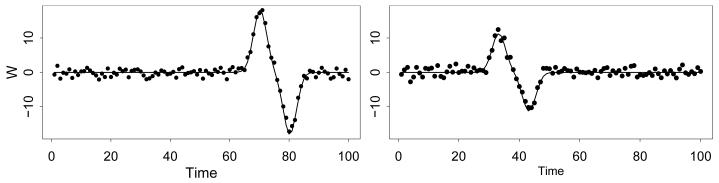
Simulated functional predictor for two subjects.

For each subject we take the outcome to be Y_i ~ N(γ_i, 5). We apply HARK and PFR to 10 simulated datasets for each sample size considered (n = 50, 100, 200, 500 subjects). For PFR, smoothed versions of the subject-specific functions are first obtained via penalized splines, and then the principal components of the smoothed functions are obtained. Between 6 and 10 principal components (PCs) are required to capture 95% of the variability in the data, depending on the simulation and the sample size n (6-8 for n = 50 and 9-10 for n = 500). Between 6 and 9 PCs are required to capture 90% of the variability. These PCs are difficult to interpret; the loading functions of two PCs for a randomly chosen simulation in the case n = 500 are shown in Figure 4.

Figure 4.

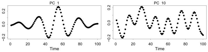
Loadings for two principal components of the simulated functional data.

Before we apply smoothing splines to estimate the coefficient function β(x) we explore the unsmoothed estimate. This estimate is shown in the left panel of Figure 5, along with point-wise 95% confidence bounds, for a randomly-chosen simulation with n = 500. The function has periodic behavior, and its interpretation is not clear.

Figure 5.

Estimated coefficient function β(x) (solid curves) and point-wise 95% confidence bounds (dotted curves) for PFR on the simulated data. Left: without smoothing. Right: with smoothing (note change in y-axis scale).

Smoothing a periodic function such as this one is questionable; however, we show the smoothed estimate of β(x) in the right panel of Figure 5. Bias-adjusted point-wise confidence bounds are also shown. A significant relationship has been detected between the predictor and the outcome, since the confidence bounds exclude zero for large portions of the domain. The smoothed estimate of β(x) suggests that high values of the predictor at the beginning of the time series, and low values of the predictor at the end of the time series, may be associated with higher values of the outcome. This effect is technically correct and is an artifact of the shape of the “blip”, namely an upward spike followed by a downward spike. However, this result does not capture the crucial fact: that the outcome is highly correlated with the magnitude of a particular feature that occurs at a variable time. Results of the Goldsmith et al. (2011) method are very similar for other sample sizes (n = 50, 100, 200). Although in this simple simulation one could use registration to align the subject-specific functions, this would not be the case in a slightly more complex example, for instance if we simulated a random number of “blips” for each subject.

To implement HARK for this example, we take ${\theta }_i=({\beta }_{0i},{\tau }_i^2,M_i,{\stackrel{‒}{\gamma }}_i,{\stackrel{‒}{\mu }}_i,{\stackrel{‒}{\sigma }}_i^2)$ as suggested in Section 3. We also use a Gaussian kernel, which is not identical to the kernel used to generate the data but can represent it accurately. To do model selection we use the maximum a posteriori estimate $\widehat{\zeta }$ of the vector ζ as described in Section 3.

The true model for this example includes the predictor ${\theta }_{i4}={\stackrel{‒}{\gamma }}_i$ and omits θ_ij for j ≠ 4. The true function g₄(θ_i4) is g₄(θ_i4) = θ_i4. The HARK results are summarized in Table 1, for the different sample sizes, with 10 simulated datasets for each sample size. Column 2 gives the percentage of simulated datasets for which HARK estimates ${\Sigma }_{p=1}^P{\zeta }_{4p}\ne 0$, i.e., for which the HARK estimated model correctly includes the predictor θ_i4. Column 3 gives the percentage of simulations in which HARK incorrectly estimates ${\Sigma }_{p=1}^P{\zeta }_{jp}\ne 0$ for some other predictor j ≠ 4 (a false positive). Column 4 reports the root mean squared error (RMSE) of the estimator of g₄, conditioning on the true model and averaging the RMSE over the domain of g₄. The percentage of that domain for which the 95% posterior bands for g₄ cover the true value is given in Column 5. The width of the posterior bands for g₄, averaged over the domain, is given in Column 6. The values in Columns 4-6 are means over the simulations, with standard deviations shown in parentheses.

Table 1.

Results of HARK in the first simulation study. Standard deviations across simulated datasets are shown in parentheses.

Sample size	% simulations w/ g4 in model	% simulations w/ gj in model, j ≠ 4	RMSE of ĝ4	Coverage of g4 95% bands	Avg. width of g4 95% bands
50	40	10	1.51 (0.49)	94.9 (8.2)	6.71 (1.03)
100	90	0	1.20 (0.28)	94.4 (7.8)	4.93 (0.61)
200	100	0	0.93 (0.09)	96.2 (6.1)	3.63 (0.28)
500	100	0	0.58 (0.13)	95.6 (6.9)	2.16 (0.12)

We see that the model selection accuracy is remarkably good: for sample sizes over 100 the estimated model is equal to the true model for all simulated datasets, while for the smaller sample sizes there are some cases in which θ_i4 is not included in the model, and only a single case in which other predictors are incorrectly included in the model. The function g₄ is also estimated accurately; the RMSE of its estimator decreases quickly as the sample size increases, and is small for all sample sizes (< 2; compare to the range of the function g₄, which is the interval (10, 20)). The coverage of the posterior bands is close to 95% for all sample sizes. The width of those bands drops quickly as the sample size increases, to a value of just 2.16 when n = 500.

In summary, the HARK model is able to detect the true relationship between the functional predictor and the outcome, even at the smallest sample sizes and with a very low false positive rate. The posterior mean estimate of g₄ is typically close to the true value of g₄, and get closer as the sample size increases. One would conclude from the HARK results that the outcome Y_i is positively associated with the magnitude of the mixture components of the predictor function f_i, which is accurate.

These conclusions are not sensitive to the choice of smoothing parameter in the empirical Bayes prior specification (Appendices A-B of the supplemental materials). Multiplying or dividing the smoothing parameter by a factor of two does not change any of the qualitative conclusions. The quantitative results after multiplying the smoothing parameter by two are nearly indistinguishable from the original results; the only change in terms of model selection results is that there are two false positives instead of one at the smallest sample size, and that for the sample size n = 100 the model selection accuracy increases to 100%. The other numerical results are nearly unchanged. When the smoothing parameter is divided by two, the model selection results are again not much affected; the only change being that the first entry of Column 2 in Table 1 decreases from 40% to 30%. The RMSE and the width of the posterior bands do increase noticeably; the RMSE increases by 26.7% on average across the simulations and sample sizes, while the width of the posterior bands increases by 10.2% on average.

5.2 Simulating from the Functional Linear Model

Next we generate data according to the functional linear model example of Goldsmith et al. (2011). The predictor functions f_i(·), noisy functional observations W_i(x_k), and scalar outcomes Y_i are generated as follows, where $x_k=\frac{k}{10}:k=0,\dots ,100$ on the interval [0, 10].

$$f_i\left(x_k\right)=u_{i1}+u_{i2}{x}_k+\sum _{\ell =1}^{10}\left[v_{i\ell 1}\sin \left(\frac{2\pi \ell }{10}{x}_k\right)+v_{i\ell 2}\cos \left(\frac{2\pi \ell }{10}{x}_k\right)\right]$$

$$W_i\left(x_k\right)\sim N\left(f_i\right(x_k),1.0)Y_i=\frac{1}{101}\sum _{k=0}^{100}{f}_i\left(x_k\right)\beta \left(x_k\right)+{\epsilon }_{i}i=1,\dots ,n.$$

Here ε_i ~ N(0, 0.25), u_i1 ~ N(0, 25), u_i2 ~ N(0, 0.04), and v_iℓ1, v_iℓ2 ~ N(0, 1/ℓ²).

Results for PFR on this example are given in Goldsmith et al. (2011), where PFR is shown to recover the true β(x) coefficient function accurately and efficiently. To implement HARK for this example, we again take ${\theta }_i=({\beta }_{0i},{\tau }_i^2,M_i,{\stackrel{‒}{\gamma }}_i,{\stackrel{‒}{\mu }}_i,{\stackrel{‒}{\sigma }}_i^2)$, and use a Gaussian kernel since it is appropriate to represent the smoothly varying predictor functions. For each of the sample sizes n = 50, 100, 200, 500 and a single simulation, HARK finds no significant relationship between the functional predictor and the outcome; repeating the simulation yields the same result. So HARK is unable to recover the function β(x), since it assumes a different model that is unrelated to the functional linear model.

6. APPLICATION TO THE SLEEP HEART HEALTH STUDY

6.1 Background

The Sleep Heart Health Study (SHHS) is a landmark study of sleep and its impacts on health outcomes. A detailed description of the SHHS can be found in Quan et al. (1997), Di, Crainiceanu, Caffo and Punjabi (2009), and Crainiceanu, Staicu and Di (2009). Between 1995 and 1997, a sample of 6, 441 participants was recruited; participants less than 65 years of age were over-sampled on self-reported snoring to augment the prevalence of sleep-disordered breathing (a condition where the airway of the throat collapses, triggering an arousal). In addition to the in-home polysomnogram (PSG), data on sleep habits, blood pressure, anthropometrics, medication use, daytime sleep tendency, and quality of life were collected. A PSG is a quasi-continuous multi-channel recording of physiological signals acquired during sleep that include two surface electroencephalograms (EEGs).

It is of interest to understand how physiological characteristics may be related to sleep patterns, as measured using the EEG data. We focus on the physiological characteristics respiratory disturbance index and body mass index. The respiratory disturbance index, or apnea/hypopnea index, is a measure of sleep-disordered breathing. The methods currently in use for relating physiological outcomes to the EEG data in the Sleep Heart Health Study are mainly based on principal component regression and penalized splines (Di et al. 2009; Crainiceanu, Caffo, Di and Punjabi 2009; Crainiceanu, Staicu and Di 2009).

We will relate the physiological characteristics to the time series of normalized δ-power, an indicator of slow neuronal firing that is a summary of the EEG signal. The δ-power time series is measured from sleep onset, and so is initially synchronized across patients. It tends to go up for all subjects in the first 30-45 minutes of sleep; this corresponds to a dominance of slow-wave brain firing characterizing the period immediately following sleep onset. As the night progresses subjects go through sleep cycles whose length, size, and number may vary across the population. Thus, subject δ-power patterns and cycles may become de-synchronized in time across subjects.

The number or magnitude of fluctuations in the time series may have physiological importance, and may be related to the outcomes. HARK is designed to capture this type of variability; while traditional approaches regress the outcome Y_i on f_i(x) for each x, HARK regresses Y_i on the parameters of kernels that can occur at variable locations. For this reason the functions f_i(·) do not have to be aligned across subjects when applying HARK, i.e. at any fixed time x the subjects can be in different parts of their sleep cycle.

For each subject we compute the normalized δ-power as described in Crainiceanu, Caffo, Di and Punjabi (2009), aggregating at the one-minute level. Figure 1 shows the resulting time series for four subjects, along with smoothed curves obtained by penalized splines.

6.2 Application of HARK

Next we use the Sleep Heart Health Study data to relate sleep patterns, as measured by the EEG time series, to respiratory disturbance index (RDI) and body mass index (BMI). We find that HARK represents the functional data both accurately and parsimoniously, and detects important and previously undescribed relationships between the sleep EEG data and both RDI and BMI.

The δ power (EEG) series are defined on a common time domain ${\mathcal{X}}_i=\mathcal{X}$ (the function domain is the first four hours of sleep; we make $\mathcal{X}$ slightly larger than this interval when applying HARK in order to mitigate edge effects). The (normalized) δ power has a range of zero to one, so we take the observations W_i(x_ik) to be the logit transformation of δ power.

HARK is applied as described in Sections 2-4, using a Gaussian kernel and taking ${\theta }_i=({\beta }_{0i},{\tau }_i^2,M_i,{\stackrel{‒}{\gamma }}_i,{\stackrel{‒}{\mu }}_i,{\stackrel{‒}{\sigma }}_i^2)$. The resulting posterior mean estimate of the function f_i is shown in the left panels of Figure 6 for two randomly selected subjects i. The estimates are similar to penalized spline estimates of the same time series, also shown. They sometimes differ substantially near the start and end of the time series, where the difference is due to the edge effects of the two estimators.

Figure 6.

Left Panels: HARK (solid curve) and penalized spline (dashed curve) functional estimates of the EEG δ-power signals for two randomly selected subjects. Right Panels: Mean line β_0i and mixture components (solid curves) from a single HARK posterior sample, for the same two subjects. The function f_i for the same posterior sample is also shown (dashed curve).

In addition to yielding similar functional estimates to other methods, the HARK functional representation is parsimonious. The right panels of Figure 6 show the function representation from a single posterior sample, for the same two subjects. The horizontal line shows the mean ${\beta }_{0i}^{\left(\ell \right)}$ for this posterior sample ℓ, and the mixture components are shown deviating from this mean line. The function $f_i^{\left(\ell \right)}$ for this posterior sample is shown as a dashed curve; it is simply the sum of ${\beta }_{0i}^{\left(\ell \right)}$ and the mixture components, this sum being expressed in (1). The function is estimated using few mixture components; for the (randomly selected) posterior sample shown in the figure $M_i^{\left(\ell \right)}$ is equal to 6 and 4, respectively, for the two subjects. The total number of parameters in the representation of f_i is 1 + 3M_i (each mixture component has three parameters), so that the number of parameters in this posterior sample is 19 and 13, respectively, for the two subjects.

For the outcome variable log BMI, the model selected by HARK includes the single predictor β_0i; for the outcome variable log RDI, the model selected includes the three predictor variables β_0i, M_i, and ${\stackrel{‒}{\gamma }}_i$. The estimated functions g_j relating these predictors to the outcome variables are shown in Figure 7, along with 95% posterior bands capturing the uncertainty in these functions. Since M_i is an integer-valued variable, the function g₃ relating it to log RDI is shown only at the discrete values where M_i is defined. In these plots we show the functions on the domain defined by the .025 and .975 quantiles of the predictor values (more precisely, on point estimates of those predictor values taken to be their posterior mean given ${\left\{W_{ik}\right\}}_{k=1}^{K_i}$). Outside of this region there is less information in the data regarding the functions gj , so the posterior bands are wide and the function estimates are primarily driven by modeling choices rather than by the data.

Figure 7.

Estimated functions g_j relating the sleep study outcome variables to the predictors. Top left: the function relating log BMI to the predictor β_0i; Clockwise from top right: the functions relating log RDI to the predictors β_0i, ${\stackrel{‒}{\gamma }}_i$, and M_i respectively.

The estimated functions are smooth, while there is some non-smoothness of the posterior bands due to having fixed the knot locations. Placing a prior distribution on the knot locations would create smoother posterior bands, at the cost of some additional computation time.

The predictor β_0i measures the average logit-δ-power; Figure 7 shows that this is negatively associated with body mass index. Additionally, respiratory disturbance index is negatively associated with the average logit-δ-power, the number of mixture components M_i, and the average magnitude ${\stackrel{‒}{\gamma }}_i$ of those mixture components. Since the kernel form is Gaussian the mixture components represent bumps or dips in the δ-power series; this means that subjects with higher RDI tend to have fewer and less pronounced fluctuations in δ-power, a measure of slow neuronal firing. This contrasts with the fact such individuals are known to have more transitions between sleep states (Swihart 2009). These results are not contradictory, in part because transitions between sleep states occur at a shorter time scale than the δ-power fluctuations.

6.3 Application of Penalized Functional Regression

For comparison we apply PFR to the sleep data. The estimated coefficient function β(·) is shown in Figure 8, for the two outcomes log RDI and log BMI. Both log RDI and log BMI are negatively associated with δ-power during the first two hours; after two hours there is no statistically significant relationship between the δ-power and the outcomes. The δ-power signals are less synchronized after two hours, attenuating the predictive power of PFR.

Figure 8.

Estimated coefficient function β(x) (solid curves) and point-wise 95% confidence bounds (dotted curves) for PFR on the sleep data. Left: log-RDI outcome variable. Right: log-BMI outcome variable.

7. CONCLUSIONS

HARK provides a method for relating continuous outcomes to functional predictors, based on a nonparametric kernel mixture representation of the predictors. It is appropriate when one hypothesizes that the functional data may include features such as bumps or plateaus occurring at varying locations and that the frequency and characteristics of those features may be related to the outcome. We introduced a novel two-stage computational method that can handle large numbers of subjects, and that propagates the uncertainty from the first into the second stage. The validity of this computational method does not rely on the specifics of the HARK model, and we are currently formulating our method for use in a large class of Bayesian models.

REFERENCES

- Best NG, Ickstadt K, Wolpert RL. Spatial Poisson regression for health and exposure data measured at disparate resolutions. Journal of the American Statistical Association. 2000;95:1076–1088. [Google Scholar]
- Bigelow JL, Dunson DB. Bayesian adaptive regression splines for hierarchical data. Biometrics. 2007;63:724–732. doi: 10.1111/j.1541-0420.2007.00761.x. [DOI] [PubMed] [Google Scholar]
- Bigelow JL, Dunson DB. Bayesian semiparametric joint models for functional predictors. Journal of the American Statistical Association. 2009;104:26–36. doi: 10.1198/jasa.2009.0001. [DOI] [PMC free article] [PubMed] [Google Scholar]
- Cardot H, Ferraty F, Sarda P. Spline estimators for the functional linear model. Statistica Sinica. 2003;13:571–591. [Google Scholar]
- Cardot H, Sarda P. Estimation in generalized linear models for functional data via penalized likelihood. Journal of Multivariate Analysis. 2005;92:24–41. [Google Scholar]
- Carlin BP, Louis TA. Bayesian Methods for Data Analysis. 3rd edn Chapman and Hall; Boca Raton, FL: 2008. [Google Scholar]
- Carroll RJ, Ruppert D, Stefanski LA, Crainiceanu CM. 2nd edn Chapman & Hall; Boca Raton, FL: 2006. [Google Scholar]
- Chappell D. Introducing the Windows Azure Platform. David Chappell and Associates; San Francisco, CA: 2010. URL: http://www.microsoft.com/windowsazure/whitepapers/ [Google Scholar]
- Clyde MA, House LL, Wolpert RL. Nonparametric models for proteomic peak identification and quantification. In: Do KA, Muller P, Vannucci M, editors. Bayesian Inference for Gene Expression and Proteomics. Cambridge University Press; 2006. pp. 293–308. [Google Scholar]
- Clyde MA, Wolpert RL. Nonparametric function estimation using overcomplete dictionaries. In: Bernardo JM, Bayarri MJ, Berger JO, Dawid AP, Heckerman D, Smith AFM, West M, editors. Bayesian Statistics 8. Oxford University Press; Oxford, UK: 2007. pp. 1–24. [Google Scholar]
- Crainiceanu CM, Caffo B, Di C, Punjabi NM. Nonparametric signal extraction and measurement error in the analysis of electroencephalographic activity during sleep. Journal of the American Statistical Association. 2009;104:541–555. doi: 10.1198/jasa.2009.0020. [DOI] [PMC free article] [PubMed] [Google Scholar]
- Crainiceanu CM, Staicu A, Di C. Generalized multilevel functional regression. Journal of the American Statistical Association. 2009;104:1550–1561. doi: 10.1198/jasa.2009.tm08564. [DOI] [PMC free article] [PubMed] [Google Scholar]
- Crainiceanu C, Reiss P. refund: Regression with Functional Data. 2011 R package version 0.1-5; URL: http://CRAN.R-project.org/package=refund.
- de Boor C. A Practical Guide to Splines. Springer-Verlag; New York: 2001. Revised Edition. [Google Scholar]
- Dey DK, Ghosh SK, Mallick BK, editors. Generalized Linear Models: A Bayesian Perspective. Marcel Dekker; New York: 2000. [Google Scholar]
- Di C, Crainiceanu CM, Caffo BS, Punjabi NM. Multilevel functional principal component analysis. Annals of Applied Statistics. 2009;3:458–488. doi: 10.1214/08-AOAS206SUPP. [DOI] [PMC free article] [PubMed] [Google Scholar]
- DiMatteo I, Genovese CR, Kass RE. Bayesian curve-fitting with free-knot splines. Biometrika. 2001;88:1055–1071. [Google Scholar]
- Donoho DL, Johnstone IM. Ideal spatial adaptation by wavelet shrinkage. Biometrika. 1994;81:425–455. [Google Scholar]
- Dunson DB. Multivariate kernel partition process mixtures. Statistica Sinica. 2010;20:1395–1422. [PMC free article] [PubMed] [Google Scholar]
- Ferraty F, Vieu P. Nonparametric models for functional data, with application in regression, time-series prediction and curve discrimination. Nonparametric Statistics. 2004;16:111–125. [Google Scholar]
- Flegal JM, Haran M, Jones GL. Markov chain Monte Carlo: Can we trust the third significant figure? Statistical Science. 2008;23:250–260. [Google Scholar]
- Gelfand AE, Smith AFM. Sampling-based approaches to calculating marginal densities. Journal of the American Statistical Association. 1990;85:398–409. [Google Scholar]
- George EI, McCulloch RE. Approaches for Bayesian variable selection. StatisticaSinica. 1997;7:339–373. [Google Scholar]
- Geweke J, Bernardo JM, Berger JO, Dawid AP, Smith AFM. Bayesian Statistics 4. Oxford University Press; Oxford: 1992. Evaluating the accuracy of sampling-based approaches to the calculation of posterior moments. [Google Scholar]
- Gilks WR, Richardson S, Spiegelhalter DJ, editors. Markov Chain Monte Carlo in Practice. Chapman and Hall; New York: 1996. [Google Scholar]
- Goldsmith J, Bobb J, Crainiceanu CM, Caffo B, Reich D. Penalized functional regression. Journal of Computational and Graphical Statistics. 2011;20:830–851. doi: 10.1198/jcgs.2010.10007. [DOI] [PMC free article] [PubMed] [Google Scholar]
- Goutis C, Fearn T. Partial least squares regression on smooth factors. Journal of the American Statistical Association. 1996;91:627–632. [Google Scholar]
- Green PJ. Reversible jump Markov chain Monte Carlo computation and Bayesian model determination. Biometrika. 1995;82:711–732. [Google Scholar]
- House LL. PhD thesis. Duke University Institute of Statistics and Decision Sciences; 2006. Non-parametric Bayesian Models in Expression Proteomic Applications. [Google Scholar]
- House LL, Clyde MA, Wolpert RL. Bayesian nonparametric models for peak identification in MALDI-TOF mass spectroscopy. Annals of Applied Statistics. 2010;5(2B):1488–1511. [Google Scholar]
- James GM. Generalized linear models with functional predictors. Journal of the Royal Statistical Society, Series B. 2002;64:411–432. [Google Scholar]
- Lang S, Brezger A. Bayesian P-Splines. Journal of Computational and Graphical Statistics. 2004;13:183–212. [Google Scholar]
- Liu F, Bayarri MJ, Berger JO. Modularization in Bayesian analysis, with emphasis on analysis of computer models. Bayesian Analysis. 2009;4:119–150. [Google Scholar]
- Lunn D, Best N, Spiegelhalter D, Graham G, Neuenschwander B. Combining MCMC with “sequential” PKPD modelling. Journal of Pharmacokinetics and Pharmacodynamics. 2009;36:19–38. doi: 10.1007/s10928-008-9109-1. [DOI] [PubMed] [Google Scholar]
- MacLehose RF, Dunson DB. Nonparametric Bayes kernel-based priors for functional data analysis. Statistica Sinica. 2009;19:611–629. [Google Scholar]
- Marx BD, Eilers PHC. Generalized linear regression on sampled signals and curves: A P-spline approach. Technometrics. 1999;41:1–13. [Google Scholar]
- McCandless LC, Douglas IJ, Evans SJ, Smeeth L. Cutting feedback in Bayesian regression adjustment for the propensity score. International Journal of Biostatistics. 2010;6(2) doi: 10.2202/1557-4679.1205. Article 16. [DOI] [PubMed] [Google Scholar]
- Müller H, Stadtmüller U. Generalized functional linear models. Annals of Statistics. 2005;33:774–805. [Google Scholar]
- Osbourne BG, Fearn T, Miller AR, Douglas S. Application of near infrared reflectance spectroscopy to the compositional analysis of biscuits and biscuit dough. Journal of the Science of Food and Agriculture. 1984;35:99–105. [Google Scholar]
- Pauler DK. The Schwarz criterion and related methods for normal linear models. Biometrika. 1998;85:13–27. [Google Scholar]
- Pillai N. PhD thesis. Duke University Department of Statistical Science; Durham, NC: 2008. Lévy Random Measures: Posterior Consistency and Applications. [Google Scholar]
- Quan SF, Howard BV, Iber C, Kiley JP, Nieto FJ, O’Connor GT, Rapoport DM, Redline S, Robbins J, Samet JM, Wahl PW. The Sleep Heart Health Study: Design, rationale, and methods. Sleep. 1997;20:1077–1085. [PubMed] [Google Scholar]
- Ramsay JO, Silverman BW. Functional Data Analysis. 2nd edn Springer; New York: 2005. [Google Scholar]
- Reiss PT, Ogden RT. Functional principal component regression and functional partial least squares. Journal of the American Statistical Association. 2007;102:984–996. [Google Scholar]
- Smith M, Kohn R. Nonparametric regression using Bayesian variable selection. Journal of Econometrics. 1996;75:317–343. [Google Scholar]
- Spiegelhalter D, Thomas A, Best N, Lunn D. WinBUGS User Manual. 2003 URL: http://www.mrc-bsu.cam.ac.uk/bugs/winbugs/manual14.pdf.
- Swihart BJ. Technical report, COBRA Preprint Series. 2009. Modeling multilevel sleep transitional data via Poisson log-linear multilevel models. Article 64. [Google Scholar]
- Tierney L. Markov chains for exploring posterior distributions (with discussion) Annals of Statistics. 1994;22:1701–1762. [Google Scholar]
- Wolpert RL, Clyde MA, Tu C. Stochastic expansions using continuous dictionaries: Lévy Adaptive Regression Kernels. Annals of Statistics. 2011;39:1916–1962. [Google Scholar]
- Woodard DB, Wolpert RL, O’Connell MA. Spatial inference of nitrate concentrations in groundwater. Journal of Agricultural, Biological, and Environmental Statistics. 2010;15:209–227. [Google Scholar]
- Yao F, Müller H. Functional quadratic regression. Biometrika. 2010;97:49–64. [Google Scholar]
Associated Data
This section collects any data citations, data availability statements, or supplementary materials included in this article.