An Integrative Bayesian Modeling Approach to Imaging Genetics

Abstract

In this paper we present a Bayesian hierarchical modeling approach for imaging genetics, where the interest lies in linking brain connectivity across multiple individuals to their genetic information. We have available data from a functional magnetic resonance (fMRI) study on schizophrenia. Our goals are to identify brain regions of interest (ROIs) with discriminating activation patterns between schizophrenic patients and healthy controls, and to relate the ROIs’ activations with available genetic information from single nucleotide polymorphisms (SNPs) on the subjects. For this task we develop a hierarchical mixture model that includes several innovative characteristics: it incorporates the selection of ROIs that discriminate the subjects into separate groups; it allows the mixture components to depend on selected covariates; it includes prior models that capture structural dependencies among the ROIs. Applied to the schizophrenia data set, the model leads to the simultaneous selection of a set of discriminatory ROIs and the relevant SNPs, together with the reconstruction of the correlation structure of the selected regions. To the best of our knowledge, our work represents the first attempt at a rigorous modeling strategy for imaging genetics data that incorporates all such features.

1 Introduction

Functional magnetic resonance imaging (fMRI) is a common tool for detecting changes in neuronal activity. It measures blood oxygenation level-dependent (BOLD) contrast that depends on changes in the regional cerebral blood-flow (rCBF). fMRI has become very popular in the neuroimaging field due to its relatively low invasiveness, absence of radiation exposure and relatively wide applicability.

Statistical methods play an important role in the analysis of fMRI data and have generated a growing literature, see for example Lindquist (2008) and Lazar (2008) for reviews on methods. Dimension reduction techniques, such as principal component analysis (PCA) and independent component analysis (ICA), and clustering algorithms are routinely applied to imaging data as a way of mapping connectivity. In the fMRI literature, connectivity refers to parts of the brain that show similarities and/or that interact with each other. In particular, anatomical connectivity deals with how different brain regions are physically connected, functional connectivity is defined as the association, or correlation, between fMRI time series of distinct voxels or regions, while effective connectivity is the directed influence of one brain region on others (Friston, 1994). Because of the high-dimensionality of the data, i.e. the large number of voxels, studies often perform region-based analyses, by looking at specific regions of interest (ROIs), or by dividing the entire brain into ROIs, for example by parcellating the brain into anatomical regions (see Tzourio-Mazoyer et al., 2002, for an example). Bayesian approaches have recently found successful applications in the fMRI field (Smith et al., 2003; Penny et al., 2005; Woolrich et al., 2004, 2009; Bowman et al., 2008; Guo et al., 2008). Also, nonparametric Bayesian methods that cluster brain regions on the basis of their connectivity patterns have been proposed (Jbabdi et al., 2009). Compared to other inferential approaches and algorithmic procedures commonly used in the analysis of fMRI data, Bayesian methods allow for a direct assessment of the uncertainties in the parameters’ estimates and, perhaps more importantly, the incorporation of prior knowledge, such as on spatial correlation among voxels and/or ROIs, into the model.

In this paper we consider a problem of imaging genetics, where structural and functional neuroimaging is applied to study subjects carrying genetic risk variants that relate to a psychiatric disorder. Our work, in particular, is motivated by a data set on subjects diagnosed with schizophrenia and healthy controls, collected as part of the the Mind Clinical Imaging Consortium (MCIC) (Chen et al., 2012), where we have available measurements on fMRI scans and single nucleotide polymorphism (SNP) allele frequencies on all participants. The fMRI data were collected during a sensorimotor task, a block-design motor response to auditory stimulation. The resulting images were realigned, normalized and spatially smoothed as customary, to remove most non-task-related sources of variability from the data (Ashby, 2011; Chen et al., 2012). Here, the fMRI information is further summarized in individual contrast images of ROI-based summary statistics, as follows. For each participant, we fit a multiple regression incorporating regressors of the stimulus and its temporal derivative plus an intercept term. The resulting coefficient estimates can be used to build individual synthetic brain maps capturing the stimulus effect at each voxel. The maps are then superimposed to a fixed template atlas, e.g. the MNI space Automated Anatomical Labeling atlas (Tzourio-Mazoyer et al., 2002), and additionally segmented into automatically labelled ROIs. Summary statistics, as the median or maximum intensity values, can be computed over the voxels included in each region (Kim et al., 2005; Etzel et al., 2009). In addition to the fMRI data, we also have available measurements on single nucleotide polymorphism (SNP) allele frequencies on all subjects. We use the genetic data as potential covariates that may affect brain function, in both healthy controls and patients with schizophrenia.

The goal of our analysis is to detect local activations, that is areas of increased BOLD signal in response to a stimulus, by selecting a subset of ROIs that explain the observed activation patterns, and to identify SNPs that might be relevant to explain such activations. Understanding how connectivity varies between schizophrenic and control subjects is of utmost importance for diagnostic purposes and therapeutic interventions. The ability to link the imaging and genetic components in the participants’ subgroups could lead to improved diagnostic tools and therapies, as it is now generally recognized that brain connectivity is affected by genetic characteristics (Colantuoni et al., 2008; Liu et al., 2009). Indeed, Chen et al. (2012) find evidence of a significant correlation between fMRI and SNP data. These authors use a two-step procedure involving a combination of PCA and ICA techniques, whereas we propose to study the association between spatial patterns and genetic variations across individuals within the coherent probabilistic framework offered by Bayesian hierarchical models.

We develop a hierarchical mixture model that includes several innovative characteristics. First, it incorporates the selection of ROIs that discriminate the subjects between schizophrenic patients and healthy controls, allowing for a direct assessment of the uncertainties in the estimates of the model selection parameters. Second, it allows the group-specific distributions to depend on selected covariates, i.e. the SNP data. In this sense, our proposed model is integrative, in that it combines the observed brain activation patterns with the subjects’ specific genetic information. Third, it incorporates prior knowledge via network models that capture known dependencies among the ROIs. More specifically, it employs spatially defined selection process priors that capture available knowledge on connectivity among regions of the brain, so that regions having the same activation patterns are more likely to be selected together. Furthermore, our hierarchical formulation accounts for additional correlation among selected ROIs that may not be captured by the network prior. Applied to the schizophrenia data set, the model allows the simultaneous selection of a set of discriminatory ROIs and the relevant SNPs, together with the reconstruction of the dependence structure of the selected regions. To the best of our knowledge, our work represents the first attempt at a rigorous modeling strategy for imaging genetics data that incorporates all such characteristics.

The remainder of the paper is organized as follows: In Section 2 we introduce our modeling framework and its major components. We describe posterior inference and prediction in Section 3. In Section 4 we first assess performances of our proposed model on simulated data and then investigate results on data from our case study on schizophrenia. We conclude the paper with some remarks in Section 5.

2 Hierarchical Bayesian Model

In its most general formulation, we depict our proposed model as a hierarchical mixture model including selection of discriminating features (e.g. ROIs), mixture components that depend on selected covariates (e.g. SNP) and network priors that capture structural dependencies among the features. The graphical formulation of the model is illustrated in Figure 1 and its major components are described below. We also summarize the hierarchical formulation of our full model in Figure 2 at the end of this Section.

Figure 1.

Graphical formulation of the proposed probabilistic model, as described in Section 2.

Figure 2.

Hierarchical formulation of the proposed probabilistic model. X denotes the n×p matrix of ROI-based measurements, Z is the n × R matrix of covariates, g is the vector of indicators of the individual group memberships and γ is the latent binary vector of discriminatory features.

2.1 A Mixture Model with Feature Selection

We represent the ROI-based summaries of BOLD signal intensity as measurements {x_ij, i = 1, …, n, j = 1, …, p} on a set of p features (the anatomical ROIs) on n subjects. We envision that some of the features could discriminate the n subjects into, say, K separate groups (e.g., schizophrenia cases and healthy controls). Therefore, we introduce a latent binary vector γ = (γ₁, …, γ_p) such that γ_j = 1 if the j-th feature is discriminatory and γ_j = 0 otherwise. By employing a discriminant analysis framework, we model the data as a mixture model of the general type

$$f_k(x_{ij}\mid {\gamma }_j)=(1-{\gamma }_j)f_0(x_{ij};{\theta }_{0j})+{\gamma }_{j}f(x_{ij};{\theta }_{kj}),k=1,\dots ,K,$$ (1)

where f₀(x_ij; θ_0j) describes the distribution of the “null” model for the non-discriminatory features, while f(x_ij; θ_kj) is the distribution of the measurements on the discriminatory features for subjects in group k. In this paper, we assume Gaussian distributions for the mixture components, that is $f_0(x_{ij};{\theta }_{0j})=N(0,{\sigma }_{0j}^2)$, and $f(x_{ij};{\theta }_{kj})=N({\mu }_{kj},{\sigma }_{kj}^2)$. Without loss of generality, we also assume that the measurement data are centered across all subjects within each feature.

Our model formulation follows an approach to feature selection in mixture models that was introduced by Tadesse et al. (2005) and Raftery and Dean (2006). These authors formulated clustering in terms of a finite mixture of Gaussian distributions with an unknown number of components and then introduced latent variables to identify discriminating features. Kim et al. (2006) proposed an alternative modeling approach that uses infinite mixture models via Dirichlet process priors. Also, Hoff (2006) adopted a mixture of Gaussian distributions where different clusters were identified by mean shifts and where discriminating features were identified via the calculation of Bayes factors. Stingo et al. (2012) extended the approach of Tadesse et al. (2005) and Raftery and Dean (2006) to the discriminant analysis framework. Building a feature selection mechanism into mixture models is a more challenging problem than in general linear settings, where the latent indicator vector γ is used to induce mixture priors on the regression coefficients. In mixture models, only the observed elements of the matrix X guide the selection and γ is used to index the contribution of the different features to the likelihood terms of the model, as in our formulation (1).

Let us now denote features indexed by γ_j = 1 as X_(γ), and those indexed by γ_j = 0 as X_(γ^c). While the former set defines a mixture distribution across the n samples, the latter favors one multivariate normal distribution across all samples. Following the finite mixture model formulation of Tadesse et al. (2005) we can write our model for sample i as

$$\begin{array}{c}{\mathbf{x}}_{i({\gamma }^c)}\mid ·~\mathcal{N}(\mathbf{0},{\mathbf{\Omega }}_{({\gamma }^c)})\\ {\mathbf{x}}_{i(\gamma )}\mid g_i=k,·~\mathcal{N}({\mathit{\mu }}_{k(\gamma )},{\mathbf{\sum }}_{k(\gamma )}),\end{array}$$ (2)

with g_i = k if the i-th sample belongs to group k. In the supervised setting, also known as discriminant analysis, in addition to the observed vectors x_i’s, the number of groups K and the classification labels g_i’s are also available and the aim is to derive a classification rule that will assign further cases to their correct groups (see Section 3.1). Here we assume diagonal variance-covariance matrices, that is, ${\mathbf{\sum }}_{k(\gamma )}=\text{Diag}({\sigma }_{k1}^2,\dots ,{\sigma }_{{kp}_{\gamma }}^2)$, with p_γ the number of non-zero elements in the vector γ, and ${\mathbf{\Omega }}_{({\gamma }^c)}=\text{Diag}({\sigma }_{01}^2,\dots ,{\sigma }_{0(p-p_{\gamma })}^2)$, and then impose inverse-gamma priors on the variance components, ${\sigma }_{kj}^2~IG({\sigma }_{kj}^2;a_k,b_k)$, k = 0, 1, …, K. Even though we make this simplifying assumption at this stage of the hierarchy, our proposed model is still able to capture structural dependencies via the specification of the prior model for the mean components that we describe in Section 2.3.2.

2.2 Covariate-Dependent Characterization of the Mixture Components

We allow the mixture components of model (2) to depend on a set of covariates. Let’s denote with Z_i = (Z_i1, …, Z_iR)^T the set of available covariates for the i-th individual. We model the means of the discriminating components as subject-specific parameters

$${\mathit{\mu }}_{ik(\gamma )}={\mathit{\mu }}_{0k(\gamma )}+{\mathit{\beta }}_{k(\gamma )}^T{\mathbf{Z}}_i,k=1,\dots ,K,$$ (3)

where μ_0k(γ) is a baseline process which captures brain connectivity (described in detail in the following Section 2.3.2) and β_k(γ) is a R × p_γ matrix of coefficients describing the effect of the covariates on the observed measurements. More in detail, our model formulation uses component-specific parameters that determine how covariates, and other relevant spatial characteristics, affect the observed measurements x_i(γ), on the n subjects, given the selected features. In this respect, the classification of the n subjects in K groups is driven by the subjects’ covariates. In particular, in our application to the schizophrenia data set the model relates the subjects’ brain activity to available information on genetic covariates.

We want to allow different covariates to affect the individual mixture components. For this we introduce spike and slab priors on β_k(γ). First, we define a binary latent indicator d_rk, r = 1, …, R, such that

$${\delta }_{rk}=\{\begin{array}{ll}1\hfill & \text{with}\text{probability}{w}_{rk}\hfill \\ 0\hfill & \text{with}\text{probability}1-w_{rk}.\hfill \end{array}$$

If δ_rk = 1, then the r-th covariate is considered relevant to explain the observed measurements in the k-th mixture component. In this case we allow the corresponding vector β_rk(γ) to be sampled from a multivariate normal prior distribution. Otherwise, the r-th covariate does not affect the response data and the corresponding regression coefficient vector β_rk(γ) is set to 0 for component k. We choose a conjugate setting and write the prior on the r-th row vector β_rk(γ), for the k-th component, as

$${\mathit{\beta }}_{rk(\gamma )}~(1-{\delta }_{rk}){\mathcal{I}}_0({\mathit{\beta }}_{rk(\gamma )})+{\delta }_{rk}\mathcal{N}({\mathbf{b}}_{0k(\gamma )},h{\mathbf{\sum }}_{k(\gamma )}),$$ (4)

where (β_rk(γ)) is a vector of point masses at zero and h > 0 some suitably large scale parameter to be chosen. Large values of h correspond to a prior well spread out over the parameters space, and typically encourage the selection of relatively large effects. We refer to Smith and Kohn (1996), Chipman et al. (2001) and O’Hara and Sillanpaa (2009) for discussions on the choice of this parameter. A Bernoulli prior on δ_rk, with parameter w_rk, completes our selection prior model on the covariates,

$$P(\mathit{\delta }\mid \mathbf{w})=\prod _{k=1}^K\prod _{r=1}^R{w}_{rk}^{{\delta }_{rk}}{(1-w_{rk})}^{1-{\delta }_{rk}}.$$

In our applications we fix the hyperparameters w_rk. Alternatively, one can place a Beta hyperprior on these parameters.

Notice that our setting allows individual covariates to have differential effects (β_r1(γ), …, β_rK(γ)) on the selected features. In the application to the schizophrenia data set, our integrative model allows the selection of SNPs that are implicated in the differential activation patterns observed in patients and healthy controls. Thus, a SNP can be correlated to a discriminatory ROI for subjects in one group, and hence help understanding the activation patterns for that group, and not be correlated to the same discriminatory ROI in the other group. This may happen if the selected ROI shows heterogeneous activation levels, explained by the selected SNP, in one group but not in the other. Our model also allows a SNP to be associated to differential activations in both groups.

2.3 Networks for Structural Dependencies

We still need to specify priors on the feature selection vector γ and on the baseline process μ_0k(γ). For those parameters we employ prior models that capture information on dependence structures.

2.3.1 A Markov Random Field for Feature Selection

The selection of the discriminatory features in our model (2) is driven by the latent variables γ_j’s. Here we impose a spatial process on γ_j that takes into account network dependencies among the features, so that dependent features are more likely to be selected together. The network structure is determined a priori on the basis of available information. In particular, in our application to the schizophrenia data set knowledge is available on the anatomical arrangement of the ROIs. We therefore construct a symmetric matrix S that captures spatial connectivity, with element {s_ij = 1} if ROI i and ROI j are directly connected in the network and with {s_ij = 0} otherwise. Although we do not pursue this option here, we notice that one could extend the definition of the matrix S to allow for entries s_ij ∈ IR⁺, that is continuous weights, to incorporate knowledge on physical distance between features, similarly to what routinely done in “auto-logistic models” (Besag, 1974) and spatial conditional (CAR) and simultaneous (SAR) autoregressive models (Banerjee et al., 2003).

We model spatial dependencies via an Ising prior model on the γ_j’s. This is a type of Markov random field (MRF), where the distribution of a set of random variables follows Markov properties that can be described by an undirected graph. Smith et al. (2003) and Penny et al. (2005) first used MRF models as prior distributions for the coefficients of voxel-based generalized linear models for fMRI data. Ising models have also recently found useful applications in genomics, to capture regulatory networks, see for example Li and Zhang (2010), Stingo et al. (2011) and Telesca et al. (2012). In a MRF, variables are represented by nodes and relations between them by edges. The Ising model is characterized by the following probabilities

$$P({\gamma }_j\mid {\gamma }_i,i\in N_j)=\frac{exp({\gamma }_{j}F({\gamma }_j))}{1+exp(F({\gamma }_j))},$$ (5)

where F (γ_j) = e + fΣ_i∈Nj (2γ_i − 1) and N_j is the set of direct neighbors of feature j in the network. The parameter e controls the sparsity of the model, while higher values of f encourage neighboring features to take on the same γ_j value. The global MRF distribution for γ can be defined up to its normalizing constant as

$$P(\mathit{\gamma }\mid e,f)\propto exp(e{\mathbf{1}}_p^T\mathit{\gamma }+f{\mathit{\gamma }}^T\mathbf{S}\mathit{\gamma }),$$ (6)

where 1_p is the unit vector of dimension p and S is the matrix capturing a priori likely connections among the nodes, as described above. Note that if a feature does not have any neighbor, then its prior distribution reduces to an independent Bernoulli, with parameter exp(e)/[1 + exp(e)], a prior often adopted in the Bayesian variable selection literature.

Following Li and Zhang (2010) and Stingo et al. (2012), we treat e and f as fixed hyperparameters. Although the parametrization is somewhat arbitrary, some care is needed in deciding whether to put a prior distribution on f. In particular, allowing f to vary can lead to a phase transition problem, that is, the expected number of variables equal to 1 can increase massively for small increments of f. This problem can happen because equation (5) can only increase as a function of the number of γ_i’s equal to 1. In variable selection, especially when p is large, phase transition leads to a drastic change in the proportion of included variables. An empirical estimate of the phase transition value can be obtained using the algorithm proposed by Propp and Wilson (1996) and the values of e and f can then be chosen accordingly. In this paper we first set e to a small value that reflects our belief in a sparse model. This value can be chosen based on the logistic transformation of e in the case of no neighbors, as a lower bound of the prior probability of feature selection. As for f, any value of f below the phase transition point can be considered a good choice, with values closer to the phase transition point leading to higher prior probabilities of selection for those nodes whose neighbors are already selected, particularly in a sparse network.

2.3.2 Component-Specific Dependencies

We complete our model with a prior specification on the baseline process μ_0k(γ) in (3). This component is a random effect capturing relevant characteristics of the selected features that affect the observed measurements x_i(γ), on the n subjects, and that are not explained by the effects of the selected covariates. In our application to the schizophrenic data set, we use this baseline process to capture additional effects on activations among selected ROIs that are not explained by the genetic covariates. In particular, we look at μ_0k(γ) as a way to capture general relationships among selected features. Correlation among distant ROIs is in fact a well described phenomenon in the fMRI literature, in addition to the dependence based on proximity, which, in our model, is captured by the MRF prior on γ (Friston, 1994).

We assume μ_0k(γ) a realization of a multivariate normal distribution,

$${\mathit{\mu }}_{0k(\gamma )}~N_{p_{\gamma }}({\mathit{\nu }}_{k(\gamma )},h_1{\mathbf{\Gamma }}_{0k(\gamma )}),k=1,\dots ,K,$$ (7)

for some fixed scale parameter h₁ > 0, and assume the precision matrix ${\mathbf{\Gamma }}_{0k(\gamma )}^{-1}$ to come from a Wishart distribution, that is, Γ_0k(γ)|δ_k, Q ~ IW (d_k, Q). Alternatively, a more general scaled inverse Wishart can be used (Gelman and Hill, 2007, Section 13.3). Notice how we define, again, component-specific parameters. This allows us to estimate component-specific dependence structures. A normal distribution on ν_k(γ) completes the prior specification.

Figure 2 summarizes the hierarchical formulation of our full model.

3 Posterior Inference

For posterior inference, our primary interest is in the selection of the discriminating features and of the covariates that affect the observed measurements, as captured by the selection vectors γ and δ. We also want to do inference on the dependence structure among the selected features. Here we design an MCMC algorithm that explores the model space for configurations with high posterior probability. These algorithms are commonly used in Bayesian variable selection settings, and have been successfully employed in genomic applications with very large number of variables (George and McCulloch, 1993, 1997; Brown et al., 1998; Tadesse et al., 2005; Stingo et al., 2011). Clearly, with large dimensions, exploring the posterior space is a challenging problem. A typical strategy relies on exploiting the sparsity of the model, i.e., the belief that most of the variables are not related to the underlying biological process. Such algorithm allows then to explore the posterior space in an effective way, quickly finding the most probable configurations, i.e., those corresponding to sets of variables with high posterior probability, while spending less time in regions with low posterior probability.

As it is typical in the implementation of MCMC methods for variable selection, to speed up the convergence of the MCMC, we integrate out some of the model parameters from the posterior distribution, specifically the variance components in (2), the regression coefficients in (3), for selected covariates, and the hyperparameters of the distribution (7) of the model intercepts. Therefore, we focus on the marginal posterior distribution of (γ, δ_k, μ_0k(γ)). We detail the MCMC implementation in the Appendix. Here, we succinctly describe our MCMC algorithm by the following three steps:

1. A Metropolis-Hastings step on γ: This step is based on the marginal posterior distribution of γ conditioned upon δ and the μ_0k(γ)’s. It consists of randomly choosing between changing the value of a single γ_j, from 0 to 1 or from 1 to 0, or swapping two γ_j’s (with opposite values). This step may imply a change in the dimensionality of the matrices Γ_0k(γ), which have been integrated out, while the parameter space of γ, i.e. {0, 1}^p, remains constant.

2. A Metropolis-Hastings step for δ_k: Similarly to the previous step, for each of the K components we randomly choose between changing the value of a single δ_rk, from 0 to 1 or from 1 to 0, or swapping two δ_rk’s with opposite values.

3. A random walk Metropolis-Hastings step on the μ_0k(γ)’s: given the selected features, we update μ_0k(γ) by proposing new values for all μ_0kj included in the model at that particular iteration, according to ${\mu }_{0kj}^{\mathit{New}}={\mu }_{0kj}^{\mathit{Old}}+\epsilon$, with ε ~ N (0, v²) for j = 1, …, p_γ and k = 1, … K, for some fixed choice of the proposal parameter v. For details on this step see the Appendix.

Posterior inference can be performed based on the MCMC output by calculating the marginal posterior probabilities of the individual γ_j’s and δ_rk’s. A simple strategy is to compute Monte-Carlo estimates by counting the number of appearances of each feature/covariate across the visited models. Important features and related covariates can be selected as those with highest posterior probabilities. Samples from the posterior distribution of μ_0k(γ) can then be used to infer correlation between selected features for each of the K groups.

Our model also allows inference on the variance components in (2) and the regression coefficients of the selected covariates in (3). More specifically, post-MCMC estimates of those parameters can be obtained by sampling (β_kj(δk), ${\sigma }_{kj}^2$) jointly from

$$p({\sigma }_{kj}^2\mid \mathbf{X},\mathbf{Z},\mathit{\gamma },{\mathit{\delta }}_k,{\mathit{\mu }}_{0k(\gamma )})~IG(a_k^{\prime },b_k^{\prime }),$$

with $a_k^{\prime }=a_k+n_k/2$ and

$$b_k^{\prime }=b_k+{({\mathbf{x}}_{jk}-{\mathbf{1}}_{n_k}{\mu }_{0jk})}^T{(h^{-1}{\mathbf{I}}_{n_k}+{\mathbf{Z}}_{k({\delta }_k)}{\mathbf{Z}}_{k({\delta }_k)}^T)}^{-1}({\mathbf{x}}_{jk}-{\mathbf{1}}_{n_k}{\mu }_{0jk})/2,$$

and where n_k is the frequency of the k-th group. Then,

$$p({\mathit{\beta }}_{kj({\delta }_k)}\mid \mathbf{X},\mathbf{Z},\mathit{\gamma },{\mathit{\delta }}_k,{\mathit{\mu }}_{0k(\gamma )},{\sigma }_{kj}^2)~N({\mathit{V}}_k{\mathbf{Z}}_{k({\delta }_k)}^T({\mathbf{x}}_{jk}-{\mathbf{1}}_n{\mu }_{0kj}),{\sigma }_{kj}^2{\mathit{V}}_k),$$

with ${\mathbf{V}}_k={({\mathbf{Z}}_{k({\delta }_k)}^T{\mathbf{Z}}_{k({\delta }_k)}+h^{-1}{\mathbf{I}}_{\mid {\delta }_k\mid })}^{-1}$ and $\mid {\mathit{\delta }}_k\mid ={\sum }_{r=1}^R{\delta }_{rk}$. The μ_0kj’s can be either set to a fixed value, like the posterior Monte Carlo mean, or integrated out in a Monte Carlo fashion via composition sampling, see Banerjee et al. (2003). Uncertainty on these parameters can be assessed via Bayesian credible intervals. Notice that, since our setting allows individual covariates to have differential effects on the selected features, some of those effects may not be significant in the final inference (for example, if the 95% Bayesian credible intervals of the corresponding β coefficients contain 0).

3.1 Prediction

Our modeling formulation allows prediction of new samples based on the selected features and covariates. The predictive distribution of a new observation x^f|z^f is used to classify the new sample into one of the K possible groups. Here x^f is the p × 1 vector of the observed features and z^f is the R×1 vector of the observed covariates for a new sample. Given a subset of selected ROIs, indicated by γ^*, and component specific subsets of selected SNP, indicated by ${\mathit{\delta }}_k^{\ast }$’s, the predictive distribution of the new observation ${\mathbf{x}}_{({\gamma }^{\ast })}^f\mid {\mathbf{z}}_{({\delta }_k^{\ast })}^f$ for class k is

$$p_k({\mathbf{x}}_{({\gamma }^{\ast })}^f\mid {\mathbf{z}}_{({\delta }_k^{\ast })}^f)=\frac{1}{(2{\pi }^{n_k/2})}{\mid {\mathbf{V}}_k^{\ast }\mid }^{-\frac{1}{2}}{\mid {\mathbf{z}}_{({\delta }_k^{\ast })}^{fT}{\mathbf{z}}_{({\delta }_k^{\ast })}^f+{\mathbf{V}}_k^{\ast -1}\mid }^{-\frac{1}{2}}\frac{{(b_k^{\prime })}^{a_k^{\prime }}}{{(b_k^f)}^{a_k^f}}\frac{\mathrm{\Gamma }(a_k^f)}{\mathrm{\Gamma }(a_k^{\prime })}$$ (8)

where

$$\begin{array}{l}{a}_k^f=a_k^{\prime }+1/2,\\ {\mathbf{V}}_k^{\ast }={({\mathbf{Z}}_{k({\delta }_k^{\ast })}^T{\mathbf{Z}}_{k({\delta }_k^{\ast })}+h^{-1}{\mathbf{I}}_{\mid {\delta }_k\mid })}^{-1},\\ b_k^f=b_k+{({\mathbf{x}}_{jk({\gamma }^{\ast })}-{\mathbf{1}}_{n_k}{\mu }_{0jk})}^T{\mathbf{Z}}_{k({\delta }_k^{\ast })}{\mathbf{V}}_k^{\ast }({\mathbf{V}}_k^{-1}-{\mathbf{V}}_k^{-1}{({\mathbf{Z}}_{k({\delta }_k^{\ast })}^T{\mathbf{Z}}_{k({\delta }_k^{\ast })}+{\mathbf{V}}_k^{-1})}^{-1}{\mathbf{V}}_k^{-1})\times \\ {\mathbf{V}}_k^{\ast }{\mathbf{Z}}_{k({\delta }_k^{\ast })}^T({\mathbf{x}}_{jk({\gamma }^{\ast })}-{\mathbf{1}}_{n_k}{\mu }_{0jk})/2+\frac{{({\mathbf{x}}_{jk({\gamma }^{\ast })}^f-{\mu }_{0jk})}^2}{2(1+{\mathbf{z}}_{({\delta }_k^{\ast })}^f{\mathbf{V}}_k{\mathbf{z}}_{({\delta }_k^{\ast })}^{fT})}.\end{array}$$

In (8) the μ_0kj’s are assumed to be set to a fixed value, for example the posterior Monte Carlo mean or median. Alternatively, one can perform a Monte Carlo integration of the μ_0kj’s using the values sampled within the MCMC algorithm. In our experience, we have not noticed any significant difference between the two approaches.

The probability that a future observation, given the observed data, belongs to the group k is then

$${\pi }_k(g^f\mid \mathbf{X},\mathbf{Z})=p(g^f=k\mid {\mathbf{x}}^f,\mathbf{X},{\mathbf{z}}^f,\mathbf{Z}),$$

where g^f is the group indicator of the new observation. By estimating the probability π_k = P (g_i = k) that one observation comes from group k as π̂_k = n_k/n, the previous distribution can be written in closed form as

$${\pi }_g(g^f\mid \mathbf{X},\mathbf{Z})=\frac{p_k({\mathbf{x}}_{({\gamma }^{\ast })}^f\mid {\mathbf{z}}_{({\delta }_k^{\ast })}^f){\widehat{\pi }}_k}{{\sum }_{i=1}^K{p}_i({\mathbf{x}}_{({\gamma }^{\ast })}^f\mid {\mathbf{z}}_{({\delta }_k^{\ast })}^f){\widehat{\pi }}_i},$$ (9)

with $p_k({\mathbf{x}}_{({\gamma }^{\ast })}^f\mid {\mathbf{z}}_{({\delta }_k^{\ast })}^f)$ the predictive distribution defined in (8), and the new sample can be classified based on this distribution, for example by assigning it to the group that has the highest posterior probability. The plug-in estimate π̂_k = n_k/n can be formally justified as an approximation under an non-informative Dirichlet prior distribution for π and training data exchangeable with future data, meaning that observations from training and validation sets arise in the same proportions from the groups, see for example Fearn et al. (2002).

4 Applications

4.1 Simulation studies

We investigate the performance of our model using simulated data. We consider simulated scenarios mimicking the characteristics of the real data that motivated the development of the model, where some of the ROIs appear to be highly correlated. We focus on situations where most of the measurements are noisy and test the ability of our method to discover relevant features in the presence of a large amount of noise. The SNP data record the number of copies of the minor allele at each locus for each individual, as a sequence of {0,1,2} values indicating the three possible genotypes at each SNP: major allele homozygote, heterozygote, and minor allele homozygote, see for example Servin and Stephens (2007) for a description of this additive coding. In our simulations, we considered the same data set used in the experimental data, described in Section 4.2. This choice was made to preserve realistic patterns of correlation (also known as “linkage disequilibrium”) across multiple SNPs. The simulation comprised a total of R = 50 covariates (SNP), only two of which were used to generate the measurements (activation profiles), as described below.

We generated a sample of 200 observations from a mixture of K = 2 multivariate normal densities, induced by 4 variables (features), as

$${\mathbf{x}}_i~I_{[1\le i\le n_1]}{\mathcal{N}}_4({\mathit{\mu }}_{01}+{\mathbf{B}}_1^T{\mathbf{Z}}_i,{\mathbf{\sum }}_1)+I_{[n_1<i\le 200]}{\mathcal{N}}_4({\mathit{\mu }}_{02}+{\mathbf{B}}_2^T{\mathbf{Z}}_i,{\mathbf{\sum }}_2),$$

with x_i = (x_i1, …, x_i4)^T, for i = 1, …, 200, and where I_[.] is the indicator function. The first n₁ = 150 samples were from the first component of the mixture, the last n₂ = 50 from the second. We then randomly divided the samples into a training set of 100 observations and a validation set of the same size. We set the elements of the 4 × 1 vector μ₀₁ to 0.8 and those of μ₀₂ to −0.8. The (2 × 4) regression coefficient matrix B_k = (β_k1, …, β_k4) determines the effects of the true covariates on the simulated activation profiles. We set B₁ = 0.8 · 1_2×4 and B₂ = 0.8 · 1_2×4. The covariance structure among the relevant features was chosen by setting the off-diagonal elements of Σ₁ and Σ₂ to 0.5 whereas the diagonal elements were set to 1. Note that the data generating process differs from our proposed model, where the correlation structure among the features is modeled at an hidden level via the baseline component. In addition to the four relevant features, we generated 100 noisy ones from a multivariate normal distribution centered at zero, with variances equal to 1 and off-diagonal elements of the covariance matrix equal to 0.1.

Our simulation comprises a total of 104 features and 50 covariates. We aim at finding the 4 discriminating features and the 2 covariates that truly relate to the response measurements. We are also interested in capturing the correlation structure among selected features. Our full prior model and the related hyperparameters are summarized in Figure 1. We report the results obtained by choosing, when possible, hyperparameters that lead to weakly informative prior distributions. In particular, we specified the priors on ${\sigma }_{0j}^2$ and ${\sigma }_{kj}^2$ by setting a₀ = a_k = 3, the minimum integer value such that the variance is defined, and b₀ = b_k = 0.1. Using the same rationale, we set d_k = 3, the minimum value such that the expectation of Σ_k exists, and Q = c I_p with c = 0.1. As for the β vectors of regression coefficients, we set the prior mean to b₀₁ = b₀₂ = 0. Similarly, we set m₁₀ = m₂₀ = 0. We then set h to 4 and h₁ to 1, to obtain fairly flat priors over the region where the data are defined; larger values of these hyperparameters would encourage the selection of only very large effects whereas smaller values would encourage the selection of smaller effects. As for the feature selection indicator, γ, we set e = −3, which corresponds to setting the expected proportion of features a priori included in the model to 5% of the total number of available ones. In this simulation study, we did not use any network structure on the prior distribution of γ, which correspond to set f = 0. This is also equivalent to assuming p(γ) as a product of independent Bernoulli distributions with expected value equal to 0.05. Finally, regarding the prior on the covariate selection indicator δ, we set w_rk = 0.05, which corresponds to setting the proportion of covariates expected a priori in the model to 5%. Parameters e and w_r influence the sparsity of the model.

We ran three MCMC samplers for 30,000 iterations with the first 1,000 discarded as burn-in. As starting points of the chain, we considered 3 different pairs of discriminatory ROIs and significant SNPs. More specifically, we assumed different starting counts of included ROIs and SNPs, i.e. 2 ROIs and 2 SNPs, 10 ROIs and 5 SNPs, and 15 ROIs and 10 SNPs, respectively. The actual ROIs and SNPs initially included were randomly selected from the set of available features and covariates. To assess the agreement of the results between the two chains, we looked at the correlation between the marginal posterior probabilities for ROI selection, p(γ_j|Z, X), and SNP selection, p(δ_lk|Z, X) for k = 1, 2. These indicated good concordance between the three MCMC chains, with pairwise correlation coefficients ranging from 0.999 to 1 for ROIs and from 0.997 to 0.998 (k = 1) and from 0.993 and 0.999 (k = 2) for SNPs. Concordance among the marginal posterior probabilities was confirmed by looking at scatter plots of the marginal probabilities across the two MCMC chains (figures not shown). We also used the Gelman and Rubin’s convergence diagnostics (Gelman and Rubin, 1992) in order to assess the convergence of the parameters μ_0kj’s to their posterior distributions. Those statistics were all below 1.1, ranging from 1.0051 to 1.0212, clearly indicating that the MCMC chains were run for a satisfactory number of iterations.

We then computed marginal posterior probabilities for feature and covariate selection, p(γ_j = 1|Z, X) and p(δ_rk = 1|Z, X), respectively. These are displayed in Figure 3, for all 104 features and the 50 covariates. All 4 relevant features were correctly identified by our model, with high posterior probability (> 0.98), while noisy features showed posterior probabilities smaller than 1%. In addition, the two relevant covariates were also selected for the first group, with p(δ_r1 = 1|Z, X) > 0.92, and one relevant covariate was selected for the second group, with p(δ_r2 = 1|Z, X) > 0.99. Sensitivity analyses with different choices of e and w_rk indicated that the posterior inference is quite robust. Specifically, our selection results were practically invariant when we let e vary between −3.5 and −2, which is equivalent to an a priori expected proportion of included features between 3% and roughly 10%, and w_rk vary between 3% and 10%. Regarding the other hyperparameters of the model, we noticed that smaller values of h would encourage the inclusion of smaller effects and that setting this parameter to 1 would lead to the inclusion of a few false positive covariates.

Figure 3.

Simulation study: Marginal posterior probabilities of inclusion for features (left) and covariates (middle and right).

Posterior distributions of the intercept parameters μ₀₁ and μ₀₂, given the selected features, indicated that parameters characterizing the two groups are clearly different. For example, Figure 4 shows the posterior distributions of the elements μ₀₁₁ and μ₀₂₁, corresponding to the first selected feature. These distributions were obtained from the MCMC output conditioning upon the inclusion of the four relevant features. Similar plots were obtained for other selected features (not shown).

Figure 4.

Simulation study: Density Kernel estimate of the posterior distribution of μ₀₁₁ and μ₀₂₁.

We estimated the dependence structure among selected features by looking at the posterior correlations among the corresponding intercepts, calculated based on the MCMC samples. These were

$$\mathit{Corr}{\mathit{\mu }}_{01}=\left(\begin{array}{cccc}1.0000& 0.5480& 0.5916& 0.4426\\ 0.5480& 1.0000& 0.6075& 0.4848\\ 0.5916& 0.6075& 1.0000& 0.4930\\ 0.4426& 0.4848& 0.4930& 1.0000\end{array}\right)$$

and

$$\mathit{Corr}{\mathit{\mu }}_{02}=\left(\begin{array}{cccc}1.0000& 0.5322& 0.5740& 0.5379\\ 0.5322& 1.0000& 0.5075& 0.4535\\ 0.5740& 0.5075& 1.0000& 0.4924\\ 0.5379& 0.4535& 0.4924& 1.0000\end{array}\right)$$

for group 1 and 2, respectively. These estimates show that our model is indeed able to capture correlation structure among selected features. Furthermore, we summarized the distance of the estimated correlation matrices from the true ones using the RV-coefficient, a measure of similarity between positive semidefinite matrices (Robert and Escoufier, 1976; Smilde et al., 2009). The RV coefficient R_V ∈ (0, 1) may be considered as a generalization of the Pearson’s coefficient of determination. For both groups 1 and 2, we got values very close to one, that is, R_V = 0.994 for Corr μ₀₁ and R_V = 0.997 for Corr μ₀₂, suggesting good agreement with the true correlation structures.

Finally, we assessed predictive performance. We used the 4 selected features and the 3 selected covariates, 2 for the first group and 1 for the second one, and classified the observations in the validation test using formula (9). Our model led to a misclassification of 26% of the subjects. Figure 5 shows the posterior probabilities of membership in group 1 for the 100 observations in the validation set, with the numbers 1 and 2 indicating the actual group membership. Units are sorted, from the highest to the lowest, within each group. Units within the boundaries of the dashed line are misclassified and provide a visual representation of the misclassification rate, whereas units above and below the solid line are correctly classified in group 1 and group 2, respectively. To assess the variability of our prediction result, we repeated our procedure over 100 splits of the data into training and validation sets. We obtained an average misclassification error of 25.2% of the units, with a 95% c.i. of (17,36)%.

Figure 5.

Simulation study: Posterior probabilities of membership in group 1 for the 100 observations in the validation set. The numbers 1 and 2 indicate the actual group membership. Units within the boundaries of the dashed line are misclassified; units above and below the solid line are correctly classified in groups 1 and 2, respectively.

For comparison, we looked into approaches that use a two-step approach, by (1) first classifying subjects based on the feature (ROIs) data only, and (2) then applying variable selection in linear models that regress the discriminatory features on the genetic covariates. In step (1) we looked at the prediction performances of the method for Bayesian variable selection in probit models of Sha et al. (2004), that use the x data and a binary response indicating the group membership of the samples. Averaging over 100 splits we obtained a misclassification error of 24.8%, with a 95% c.i. of (19,32)%. Also, an alternative classification method, based on support vector machine (SVM) (Cristianini and Shawe-Taylor, 2000), resulted in a misclassification error of 27.8%, with a 95% c.i. of (21,36)%. In step (2), to avoid selection biases, we used the truly discriminatory features as response variables. We applied the method of Guan and Stephens (2011), separately for each group of subjects and each feature, and compared the results with our joint estimation method. Recall that our method identified 3 true and no false significant SNPs. In general, the method by Guan and Stephens (2011) led to more false positives (FP). For example, a threshold of .5 on the marginal posterior probability of inclusion led to 2 true positives (TP) and 2 FP for feature 13 in the control group and feature 20 in the schizophrenia group, and 2 TP and 1 FP for feature 83 in the control group and feature 13 in the schizophrenia group. These results suggest that our joint selection scheme performs comparably to single-step methods in retrieving true discriminatory features but leads to a more reliable identification of the true significant SNPs.

4.2 Case study on schizophrenia

Schizophrenia is a severe psychiatric disorder that disrupts normal thinking, speech, and behavior. It has a strong genetic component with heritability estimated up to 80% based on family and twin studies (Cardno and Gottesman, 2000). Recently, there have been increasing efforts to utilize fMRI and examine genetic variation to study potential schizophrenia biomarkers, in order to better understand the pathology of schizophrenia. See Colantuoni et al. (2008), Meda et al. (2010) and Liu et al. (2009), among others. Here we have available imaging data on activation profiles captured with fMRI during a sensorimotor task for n = 210 subjects, of which n₁ = 118 are healthy controls and n₂ = 92 are subjects affected by schizophrenia. Participant recruitment and data collection were conducted by the Mind Clinical Imaging consortium (MCIC), a collaborative effort of four research teams from Boston, Iowa, Minnesota and New Mexico. Prior to inclusion in the study, all healthy participants were screened to ensure that they were free of any medical, neurological or psychiatric illnesses, including any history of substance abuse. Additional information, including participants demographics, can be found in Chen et al. (2012).

The original fMRI data were collected from all participants at four MCIC sites during a sensorimotor task, a block-design motor response to auditory stimulation. The data were then preprocessed in SPM5 (http://www.fil.ion.ucl.ac.uk/spm). In order to correct for the subject movements during the experiment, images were realigned using the INRIAlign algorithm in Freire et al. (2002). Data were then spatially normalized into the standard Montreal Neurological Institute space (Friston et al., 1995a) and resliced to 3 × 3 × 3 mm, resulting in 53 × 63 × 46 voxels. Spatial smoothing was further applied with a 10 mm Gaussian kernel. Following Chen et al. (2012), a multiple regression model was fit to the data from each participant, incorporating regressors of the stimulus and its temporal derivative plus an intercept term. The resulting regression coefficient values were used to create stimulus-on versus stimulus-off contrast images, which are sometimes also referred to as statistical parametric maps (Friston et al., 1995b). All the voxels with missing measurements were excluded. In this work, we additionally segmented the individual contrast images into p = 116 regions of interest (ROI) according to the MNI space Automated Anatomical Labeling (AAL) atlas of Tzourio-Mazoyer et al. (2002). Finally, we summarized activations in each region by computing the median of the statistical parametric map values for that region. The individual region based summary statistics were also centered by subtracting the overall mean within the region. In addition to the imaging data, we have available measurements on R = 81 genetic covariates (SNP) for each participant in the study. The SNPs were selected by accessing the schizophrenia research forum (http://www.schizophreniaforum.org/) and identifying SNPs which had been previously implicated in schizophrenia.

The goal of the MCIC study was to identify a subset of ROIs with discriminating activation patterns and a set of SNPs that are relevant to explain the ROI’s activations. Chen et al. (2012) applied a two-step procedure involving principal components (PCA) and independent component analysis (ICA) and found a significant correlation between fMRI data and the genetic covariates in both cases and controls. Here we use our unified modeling framework to relate the patterns of observed brain activity in subjects with different conditions to the individuals’ specific genome. Our model jointly infers discriminating activation patterns and identifies genetic features related to those patterns.

We split the observations into a training set and a validation set. Given the high complexity of the scientific problem we want to study, we decided to allocate a larger number of the observations to the training set. Specifically we randomly assigned 174 participants to the training set and 36 participants to the validation set. In order to obtain a training set with enough information on both groups we followed a balanced allocation scheme and randomly assigned to this set 87 subjects from the control group and the same number of subjects affected by schizophrenia.

For this data analysis we constructed a spatial network among ROIs based on the physical location of the regions in the brain. The spatial coordinates, in a three dimensional space, of the centroids of the individual regions allowed us to calculate a distance matrix among ROIs, based on the Euclidean distance. Given such matrix we constructed a spatial network by including an edge in the network if the distance between the corresponding pair of ROIs was less than a given threshold. We selected the threshold value such that the average number of neighbors was approximately 5, therefore reproducing an overall connectivity close to the one of a 3D lattice structure. We used the resulting network for the specification of the MRF prior (6) on γ. The result is a spatially based selection process of the regions of interest that enables sparsity in the resulting network structure.

Results we report below were obtained by combining the outputs from three MCMC chains. For each chain, we randomly selected different discriminatory ROIs and significant SNPs as starting points. More specifically, we initially assumed 2 ROIs and 2 SNPs, 10 ROIs and 5 SNPs, and 15 ROIs and 10 SNPs as initial counts of selected features and SNPs. We used 200,000 iterations with a burn-in of 1,000 iterations. We set the hyperparameter of the Markov random field that controls the sparsity at the ROI level to e = −4.5, which corresponds to setting the proportion of ROIs expected a priori $h_1^{\ast }=1$to be included in the model to at least 1.1% of the total number of ROIs. We considered two values for f, setting this parameter to either 0.1 or 0.5, representing a very small or a moderate effect of the prior information, respectively. For example, for f = 0.1 the prior probability of inclusion of an ROI with five of its neighbors already selected is 1.8%, that 1.6 times the prior probability of an ROI that does not have any of its neighbors selected, while for f = 0.5 the same probability is 11.9%, that is 10.8 times the probability of an ROI with no neighbors selected. These small to moderate effects allow the data to mostly drive the selection. For the SNP selection, we set w_r = 0.1, indicating that a priori approximately 10% of the SNPs are expected to be selected. In addition, although several susceptibility genes have been identified from linkage and association studies, the associations between a diagnosis of schizophrenia and individual polymorphisms have been often found weak (Harrison and Owen, 2003; Duan et al., 2010). We therefore set , favoring the selection of small SNP effects. For the other hyperparameters, we used the same settings as described in Section 4.1.

The trace plots for the number of included ROIs and SNPs showed good mixing (figures not shown). The MCMC samplers mostly visited models with 10–15 ROIs and 1–3 SNPs, indicating that the data mostly determine the amount of sparsity in the model, since overall the numbers of selected ROIs and SNPs were not close to the corresponding expected numbers a priori. We assessed the agreement of the results between the two chains by looking at the correlation coefficients between marginal posterior probabilities for ROI selection, p(γ_j|Z, X), and SNP selection, p(δ_lk|Z, X) for k = 1, 2. These indicated good concordance between the three MCMC chains, with pairwise correlation coefficients ranging from 0.998 to 0.999 for ROIs and from 0.998 to 0.999 (k = 1) and from 0.994 to 0.998 (k = 2) for SNPs, in the case f = 0.5; and from 0.996 to 0.998, from 0.997 to 0.999, and from 0.998 to 0.999, respectively, for f = 0.1. Also, the Gelman and Rubin’s statistics, calculated on the sample values of the μ_0kj’s, ranged from 1.0001 to 1.0043, indicating that our chains converged to the posterior distribution.

Posterior probabilities for all ROIs and SNPs are summarized in Figures 6 and 8, respectively. These probabilities can be used to prioritize the relevant ROIs and SNPs for further experimental work. Brain regions with high posterior probability are listed in Table 1, both for f = 0.5 and f = 0.1. As it is evident from the table, the lists of selected ROIs under the two settings largely overlapped. A threshold of 0.5 on the marginal posterior probabilities selected a subset of 5 ROIs in the case f = 0.5 and 4 ROIs for f = 0.1. This threshold corresponds to an expected false discovery rate (Bayesian FDR) of 4.8% for f = 0.5 and 3.1% for f = 0.1, which we calculated according to the formulation suggested by Newton et al. (2004). The increase in the posterior probability of ROI 5 in the first row of Table 1 is an effect of the MRF prior, since ROI 5 is connected to ROIs 21, 27 and 28. The selected ROIs, shown in Figure 7, were all mid-line frontal regions, and mostly connected in the MRF prior. The frontal superior orbital, olfactory and rectus regions have all reported schizophrenia deficits, see Nakamura et al. (2008), Diaz et al. (2011) and Langdon et al. (2011), among many others. The left frontal region included the Brodmann area 10, identified by the cross-hair in Figure 7, which is often implicated in schizophrenia (Vogeley et al., 2003; Camchong et al., 2008; Schneiderman et al., 2011).

Figure 6.

Schizophrenia data set: Marginal posterior probabilities of inclusion for ROIs for f = 0.1 (o) and f = 0.5 (+).

Figure 8.

Schizophrenia data set: Marginal posterior probabilities of inclusion for SNPs for f = 0.1 (o) and f = 0.5 (+).

Table 1.

Schizophrenia data set: List of selected ROIs and SNPs and corresponding posterior probabilities.

ROI	Name	p(γj|Z, X) for f = 0.1	p(γj|Z, X) for f = 0.5
ROI 5	Frontal Sup Orb L	0.37	0.77
ROI 21	Olfactory L	1.00	1.00
ROI 22	Olfactory R	1.00	1.00
ROI 27	Rectus L	0.95	1.00
ROI 28	Rectus R	0.93	0.99
Schizophrenia
SNP	Name	p(δ2l|Z, X) for f = 0.1	p(δ2l|Z, X) for f = 0.5
SNP 25	rs1934909	0.52	0.48
SNP 31	rs875462	0.93	0.84
SNP 44	rs17101921	0.86	0.86
Control
SNP	Name	p(δ1l|Z, X) for f = 0.1	p(δ1l|Z, X) for f = 0.5
SNP 16	rs6794467	0.98	0.99
SNP 50	rs2421954	0.99	0.99
SNP 70	rs2270641	0.99	0.99

Figure 7.

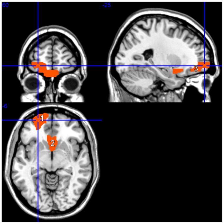
Schizophrenia data set: Map of brain network for the identified ROIs. The highlighted regions are the orbital part of the superior frontal gyrus (ROI 5, coded as ’1’, spanning superior frontal gyrus, middle frontal gyrus, inferior frontal gyrus), the olfactory cortex (ROIs 21 and 22, coded as ’2’, spanning subcallosal gyrus and anterior cingulate) and the gyrus rectus (ROIs 27 and 8, coded as ’3’, spanning medial frontal gyrus, rectal gyrus and superior frontal gyrus).

Posterior inference on the intercept parameters μ₀₁ and μ₀₂, given the selected features, and estimates of their correlations can give us indication on characteristic features of the two groups of participants and on dependence structures among selected ROIs suggesting new activation patterns. Estimated correlations for the case f = 0.5 were

$${\mathit{Corr}}_{\mu 01}=\left(\begin{array}{ccccc}1.0000& 0.0149& 0.0267& 0.0295& 0.0328\\ 0.0149& 1.0000& 0.0246& 0.0293& 0.0235\\ 0.0267& 0.0246& 1.0000& 0.0373& 0.0506\\ 0.0295& 0.0293& 0.0373& 1.0000& 0.0539\\ 0.0328& 0.0235& 0.0506& 0.0539& 1.0000\end{array}\right)$$

and

$${\mathit{Corr}}_{{\mu }_{02}}=\left(\begin{array}{ccccc}1.0000& 0.3532& 0.3403& 0.3310& 0.3562\\ 0.3532& 1.0000& 0.4509& 0.4193& 0.4227\\ 0.3403& 0.4509& 1.0000& 0.3617& 0.4024\\ 0.3310& 0.4193& 0.3617& 1.0000& 0.3818\\ 0.3562& 0.4227& 0.4024& 0.3818& 1.0000\end{array}\right)$$

for control and schizophrenic groups, respectively, showing higher correlations among ROIs in the healthy control group. This finding is consistent with previous work in fMRI, which has shown less unique brain activity in cases versus controls, and supports the presence of a generalized cognitive deficit (Calhoun et al., 2006). Similar correlations were obtained for f = 0.1.

Table 2 reports estimates and 95% credible intervals of the regression coefficients β_jk corresponding to the selected SNPs, for the selected ROIs (case f = 0.5), in the two groups of participants. Again, our findings are supported by other studies in the literature. Among those SNPs identified in the schizophrenia group, SNP 25 is in gene DISC1 on chromosome 1, a gene which is disrupted in schizophrenia (Kim et al., 2012; Kang et al., 2011). Also, SNP 31 in gene DTNBP1 on chromosome 6 has been found associated with schizophrenia (Duan et al., 2007). Interestingly, Colantuoni et al. (2008) report age-related changes in the expression of putative schizophrenia genes, including, DISC1 and DTNBP1, in the human prefrontal cortex, including Brodmann area 10. SNP 44 is on chromosome 10 and it has also been associated to schizophrenia (O’Donovan et al., 2009). This locus was identified via a Genome-wide Association study (GWA) analysis and has not yet been assigned to a specific gene. As for the control group, SNP 16 is in gene CLDN11 on chromosome 3 and SNP 70 in gene SLC18A1 on chromosome 8. Both genes are implicated in the functioning of the central nervous system (CNS) (Lal-Nag and Morin, 2009) (Lohoff et al., 2008a,b). Together with the peripheral nervous system, the CNS has a fundamental role in the control of behavior.

Table 2.

Schizophrenia data set: Posterior mean (and 95% credible interval) of regression coefficients β_jk for the selected SNPs on the selected ROIs (f = 0.5).

ROI	Name	Schizophrenia group	Control Group
		SNP 25	SNP 16
ROI 5	Frontal Sup Orb L	0.0714 (−0.0794,0.2221)	−0.1854 (−0.3175, −0.0534)
ROI 21	Olfactory L	0.0659 (−0.1029, 0.2347)	−0.2819 (−0.4444, −0.1193)
ROI 22	Olfactory R	0.0664 (−0.1041, 0.2368)	−0.2779 (−0.4172, −0.1386)
ROI 27	Rectus L	0.2341 (0.0443, 0.4238)	−0.2712 (−0.4394, −0.1031)
ROI 28	Rectus R	0.1662 (−0.0202, 0.3527)	−0.2915 (−0.4347, −0.1483)
		SNP 31	SNP 50
ROI 5	Frontal Sup Orb L	0.0192 (−0.0631, 0.1016)	0.2054 (0.0541, 0.3568)
ROI 21	Olfactory L	0.1416 (0.0494, 0.2338)	0.3275 (0.1412, 0.5137)
ROI 22	Olfactory R	0.1392 (0.0461, 0.2324)	0.2471 (0.0874, 0.4068)
ROI 27	Rectus L	0.1022 (−0.0015, 0.2059)	0.2245 (0.0318, 0.4172)
ROI 28	Rectus R	0.0753 (−0.0266, 0.1771)	0.2449 (0.0808, 0.4090)
		SNP 44	SNP 70
ROI 5	Frontal Sup Orb L	0.1013 (−0.0987, 0.3014)	0.1824 (0.0356, 0.3292)
ROI 21	Olfactory L	0.2002 (−0.0239, 0.4243)	0.2487 (0.0680, 0.4293)
ROI 22	Olfactory R	0.2293 (0.0031, 0.4556)	0.2797 (0.1249, 0.4346)
ROI 27	Rectus L	0.2398 (−0.0120, 0.4917)	0.2913 (0.1044, 0.4781)
ROI 28	Rectus R	0.2585 (0.0111, 0.5060)	0.2663 (0.1071, 0.4254)

Estimates of the regression coefficients reported in Table 2 inform us on the effects of the selected SNPs on the activations of the selected ROIs. The corresponding 95% credible intervals, also reported in the same table, allow us to assess uncertainty on those parameters. As emphasized at the end of Section 2.2, a meaningful interpretation of these regression coefficients needs to take into account the nature of the dependent variable in the regression models, which is the set of discriminatory ROIs in the two groups. An interesting feature of our results is that, while effects are all significant across selected ROIs in the control group, differential effects are clearly indicated in the schizophrenia group. For example, SNP 25 (rs1934909 in gene DISC1) has a significant effect on the Rectus L ROI only and SNP 31 (rs875462 in gene DTNBP1) on the Olfactory ROIs only. A close look at the alleles frequencies of the selected SNPs in the schizophrenia and control groups revealed that the selection is not driven by differences in genotype variation within groups. These findings call for further experimental validation.

Our model also showed good predictive performance. For f = 0.5, using all 6 selected ROIs and the selected SNP, the model misclassified 12 of the 36 samples, that is 33%, of the validation set. Similarly for the case f = 0.1. As with the simulation study, we compared our results with methods that use a two-step approach, first classifying subjects based on the imaging data only, and then applying variable selection in regression models that regress the discriminatory ROIs on the genetic covariates. In the first step, the method of Sha et al. (2004) misclassified 22 out of the 36 samples, that is 61%, and the SVM method 25 out of the 36 samples, that is 69%. In the second step, we used the 5 ROIs selected by our method as response variables and applied the method of Guan and Stephens (2011) separately for each group of subjects and each ROI. Using a threshold of .5 on the marginal posterior probability of inclusion, none of the SNPs were identified in the control group, while in the schizophrenia group the method selected SNP9 for ROI5 (p=0.53), SNP47 for ROI21 (p=0.77) and SNP21 for ROI22 (p=0.62).

5 Concluding Remarks

We have presented a hierarchical modeling framework for the analysis of data that arise in imaging genetics. Focusing on the relationships between genetic factors and brain functional patterns, we have analyzed data from a study where the interest lies in identifying brain regions (ROIs) with discriminating activation patterns between schizophrenic patients and healthy controls, and in relating the observed activation patterns with available genetic information on the subjects (SNPs). As patterns of brain connectivity in fMRI scans are known to be related to the subjects’ genome, the ability to model the link between the imaging and genetic components could indeed lead to improved diagnostics and therapeutic interventions. Overall, our results have confirmed the complex nature of genetic effects on the functional brain abnormality in schizophrenia. Particularly, the identified SNPs have implicated the DISC1 and DTNBP1 genes, associated to schizophrenia, as well as genes associated with the central nervous system, and appear to be related mainly to the frontal regions including the Brodmann area 10.

The hierarchical model we have developed has several innovative characteristics: It is integrative, in that it combines activation patterns with genetic information on the subjects; it achieves the simultaneous selection of a set of discriminatory regions and relevant SNPs; it employs spatially based selection process priors that capture available knowledge on connectivity among regions of the brain, so that regions having the same activation patterns are more likely to be selected together. An additional feature of our model is that it takes into account correlation among selected ROIs, as captured by the covariance matrices of the distribution of the intercept parameters.

Our integrative model aims at selecting SNPs that are implicated in the differential activation patterns observed in patients and healthy controls. In our analysis we have considered a relatively small set of SNPs that were already known to be of interest based on previous studies. Typically, the initial list of potentially interesting SNPs can be the result of genome-wide association (GWAS) studies, where the outcome, i.e. the known phenotype (disease/not disease), is related to the genetic covariates (SNPs) in a logistic model. Our model can then be used to determine if the selected SNPs are additionally significantly associated to an alteration of the normal brain functions. Clearly, discovery of new associations between SNPs and the disease under study is also possible with our model. In such situations, analyses with large number of SNPs can be tackled by considering gene-based summaries of SNP data. Indeed, more and more GWAS studies confirm the involvement of aggregates of common SNPs that collectively account for a substantial proportion of variation in risk to the disorder, see Purcell et al. (2009) for a schizophrenia study.

Several extensions of our model are worth investigating. First, we can learn about the fixed hyperparameters. For example, we can assume prior distributions for the parameters of the Ising model, as in Liang (2010) and Stingo et al. (2011), as well as the scale parameters of the spike and slab priors (4), as sometimes done in Bayesian variable selection, (Chipman et al., 2001; Scott and Berger, 2010). Second, extensions to mixture models for clustering the subjects are possible. In particular, infinite mixture models can be fit based on the Dirichlet process, as in Kim et al. (2006), or based on the probit stick breaking process proposed by Chung and Dunson (2009) for a mixture of univariate regression models, which also incorporates selection of the covariates. Furthermore, even though our method already suggests connections among distant features that can form new activation patterns, a more formal approach could assume μ_0k(γ) to be a realization of a network of connected components (nodes) that describes general relationships among the selected features as

$${\mathit{\mu }}_{0k(\gamma )}\mid G_{k(\gamma )}~N_{p_{\gamma }}({\mathit{\nu }}_{k(\gamma )},{\mathbf{\Gamma }}_{0k(\gamma )}),k=1,\dots ,K,$$ (10)

with G_k(γ) the graph encoding the relationships, see Dobra et al. (2011). This would allow us to estimate component-specific networks among selected ROIs. Finally, another interesting avenue is to extend our model to handle data observed at different time points. Hidden Markov models can be employed. For example, in an application to genomic data, Gupta et al. (2007) consider a hierarchical Bayesian hidden Markov regression model for determining groups of genes being influenced by separate sets of covariates over time.

Appendix: MCMC algorithm

We start by writing the expression of the marginal posterior distribution of (γ, δ_k, μ_0k(γ)) explicitly. The dimension of μ_0k(γ) varies depending on the number of non-zero components in γ. This type of issues have been traditionally addressed in the context of transdimensional MCMC algorithms. In this paper, we follow the hybrid Gibbs/Metropolis approach discussed in Dellaportas et al. (2002), based on Carlin and Chib (1995), and assume a pseudo-prior for the parameter μ_0k^c) of the non-selected features, that is μ_0k(^c) ~ N (0, Γ_0k(^c)), where ${\mathbf{\Gamma }}_{0k({\gamma }^c)}=\mathit{diag}({\sigma }_{p_{\gamma }+1}^2,\dots ,{\sigma }_p^2)$, with ${\sigma }_j^2~IG({\stackrel{\sim }{a}}_j,{\stackrel{\sim }{b}}_j)$, j = p_γ + 1, …, p. Alternatively, methods based on mixtures of singular distributions could be usefully employed in this setting (Petris and Tardella, 2003; Gottardo and Raftery, 2008). For a review of available transdimensional MCMC algorithms, we refer, among others, to Fruhwirth-Schnatter, 2006, chapter 5, and the discussion in Fan and Sisson (2011).

The un-normalized full conditionals can be derived from the conditional independencies of our model, see Figure 1. Let μ_0k = (μ_0k(γ), μ_0k(γ^c)). Then, the joint marginal posterior distribution of (γ, δ_k, μ_0k) is

$$\begin{array}{l}p(\mathit{\gamma },{\mathit{\delta }}_k,{\mathit{\mu }}_{0k}\mid \mathbf{X},\mathbf{Z})\propto {\prod }_{j:{\gamma }_j=0}p({\mathbf{x}}_{j({\gamma }^c)}\mid \mathit{\gamma }){\prod }_{j:{\gamma }_j=1}{\prod }_{k=1}^{K}p({\mathbf{x}}_{jk(\gamma )}\mid {\mathbf{Z}}_{k({\delta }_k)},{\mu }_{0jk},\mathit{\delta },\mathit{\gamma })\\ \times {\prod }_{k=1}^K\left[p({\mathit{\mu }}_{0k(\gamma )}\mid \mathit{\gamma }){\prod }_{j:{\gamma }_j=0}p({\mu }_{0jk({\gamma }^c)}\mid \mathit{\gamma })\right]p(\mathit{\gamma })p(\mathit{\delta })\end{array}$$

with

$$\begin{array}{l}p({\mathbf{x}}_{j({\gamma }^c)}\mid \mathit{\gamma })={\left(\frac{1}{\sqrt{2\pi }}\right)}^n\frac{\mathrm{\Gamma }(a_0^{\prime })}{\mathrm{\Gamma }(a_0)}\frac{b_0^{a_0}}{{b_0^{\prime }}^{a_0^{\prime }}},\\ p({\mathbf{x}}_{jk(\gamma )}\mid {\mathbf{Z}}_{\mathbf{k}({\delta }_{\mathbf{k}})},{\mu }_{\mathbf{0}\mathbf{jk}},\mathit{\delta },\mathit{\gamma })={\left(\frac{1}{\sqrt{2\pi }}\right)}^{n_k}\frac{\mathrm{\Gamma }(a_k^{\prime })}{\mathrm{\Gamma }(a_k)}\frac{{b_k}^{a_k}}{{b_k^{\prime }}^{a_k^{\prime }}}\mid {\mathbf{Z}}_{k({\delta }_k)}{\mathbf{Z}}_{k({\delta }_k)}^T+h^{-1}{\mathbf{I}}_{n_k}\mid ,\\ p({\mathit{\mu }}_{0k(\gamma )}\mid \mathit{\gamma })={\pi }^{-\frac{p_{\gamma }}{2}}{h}_1^{\ast \frac{-p_{\gamma }}{2}}\frac{{\mid \mathbf{Q}\mid }^{(d_k+p_{\gamma }+1)/2}}{{\mid \mathbf{Q}+({\mathit{\mu }}_{0k}-{\mathbf{m}}_{0k}){({\mathit{\mu }}_{0k}-{\mathbf{m}}_{0k})}^T\mid }^{(d_k+p_{\gamma })/2}}\frac{\mathrm{\Gamma }((d_k+p_{\gamma })/2)}{\mathrm{\Gamma }((d_k+p_{\gamma }+1)/2)},\\ p({\mu }_{0jk({\gamma }^c)}\mid \mathit{\gamma })=\left(\frac{1}{\sqrt{2\pi }}\right)\frac{{\stackrel{\sim }{b}}_j^{{\stackrel{\sim }{a}}_j}}{{\stackrel{\sim }{b}}_{jk}^{\prime {\stackrel{\sim }{a}}_j^{\prime }}}\frac{\mathrm{\Gamma }({\stackrel{\sim }{a}}_j^{\prime })}{\mathrm{\Gamma }({\stackrel{\sim }{a}}_j)},\end{array}$$

and where $h_1^{\ast }=2h_1$, Z_k(δ) is the n_k × |δ_k| data matrix of the selected covariates, n_k is the number of subjects allocated to the k-th component and $\mid {\mathit{\delta }}_k\mid ={\sum }_{r=1}^R{\delta }_{rk}$, and with

$$\begin{array}{l}{b}_0^{\prime }=b_0+\frac{{\mathbf{x}}_j^T{\mathbf{x}}_j}{2},\\ a_0^{\prime }=a_0+n/2,\\ b_k^{\prime }=b_k+{({\mathbf{x}}_{jk}-{\mathbf{1}}_{nk}{\mu }_{0jk})}^T{(h^{-1}{\mathbf{I}}_{n_k}+{\mathbf{Z}}_{k({\delta }_k)}{\mathbf{Z}}_{k({\delta }_k)}^T)}^{-1}({\mathbf{x}}_{jk}-{\mathbf{1}}_{n_k}{\mu }_{0jk})/2,\\ a_k^{\prime }=a_k+n_k/2,\\ {\stackrel{\sim }{a}}_j^{\prime }={\stackrel{\sim }{a}}_j+1/2,\\ {\stackrel{\sim }{b}}_{jk}^{\prime }={\stackrel{\sim }{b}}_j+\frac{{({\mu }_{0jk}-m_{0jk})}^2}{2},\end{array}$$

for k = 1, …, K and j = p_γ + 1, …, p, with x_j the n × 1 vector of the observed values for feature j and x_jk the n_k × 1 vector of the observed values for feature j and group k.

Our MCMC algorithm comprises the following three steps:

1. A Metropolis-Hastings step on γ: It consists of randomly choosing between changing the value of a single γ_j (either 0 to 1 or 1 to 0) or swapping two γ_j’s (with opposite values). The transition from the current value γ^O to the proposed value γ^N is accepted with probability

   $$min\left[\frac{{\prod }_{j:{\gamma }_j=0}p({\mathbf{x}}_{j({\gamma }^c)}\mid {\mathit{\gamma }}^N){\prod }_{j:{\gamma }_j=1}{\prod }_{k=1}^{K}p({\mathbf{x}}_{jk(\gamma )}\mid {\mu }_{0jk},\mathit{\delta },{\mathit{\gamma }}^N){\prod }_{k=1}^K\left[p({\mathit{\mu }}_{0k(\gamma )}\mid {\mathit{\gamma }}^N){\prod }_{j:{\gamma }_j=0}p({\mu }_{0jk({\gamma }^c)}\mid {\mathit{\gamma }}^N)\right]p({\mathit{\gamma }}^N)}{{\prod }_{j:{\gamma }_j=0}p({\mathbf{x}}_{j({\gamma }^c)}\mid {\mathit{\gamma }}^O){\prod }_{j:{\gamma }_j=1}{\prod }_{k=1}^{K}p({\mathbf{x}}_{jk(\gamma )}\mid {\mu }_{0jk},\mathit{\delta },{\mathit{\gamma }}^O){\prod }_{k=1}^K\left[p({\mathit{\mu }}_{0k(\gamma )}\mid {\mathit{\gamma }}^O){\prod }_{j:{\gamma }_j=0}p({\mu }_{0jk({\gamma }^c)}\mid {\mathit{\gamma }}^O)\right]p({\mathit{\gamma }}^O)},1\right].$$
2. A Metropolis-Hastings step for δ_k: Similarly to the previous step, for each of the K components we randomly choose between changing the value of a single δ_rk or swapping two δ_rk’s with opposite values. The transition from the current value ${\mathit{\delta }}_k^O$ to the proposed value ${\mathit{\delta }}_k^N$ is accepted with probability

   $$min\left[\frac{{\prod }_{j:{\gamma }_j=1}p({\mathbf{x}}_{jk(\gamma )}\mid {\mu }_{0jk},{\mathit{\delta }}_k^N,\mathit{\gamma })p({\mathit{\delta }}_k^N)}{{\prod }_{j:{\gamma }_j=1}p({\mathbf{x}}_{jk(\gamma )}\mid {\mu }_{0jk},{\mathit{\delta }}_k^O,\mathit{\gamma })p({\mathit{\delta }}_k^O)},1\right].$$
3. A random walk Metropolis-Hastings step on the μ_0k(γ)’s: We update μ_0k(γ) by proposing new values for all μ_0kj included in the model at that particular iteration, according to ${\mu }_{0kj}^N={\mu }_{0kj}^O+\epsilon$, with ε ~ N (0, v²) for j = 1, …, p_γ and k = 1, … K, for some fixed choice of the proposal parameter v. The transition from ${\mu }_{0kj}^O$ to ${\mu }_{0kj}^N$ is accepted with probability

   $$min\left[\frac{p({\mathbf{x}}_{jk(\gamma )}\mid {\mu }_{0jk}^N,\mathit{\delta },\mathit{\gamma })p({\mathit{\mu }}_{0k(\gamma )}^N\mid \mathit{\gamma })}{p({\mathbf{x}}_{jk(\gamma )}\mid {\mu }_{0jk}^O,\mathit{\delta },\mathit{\gamma })p({\mathit{\mu }}_{0k(\gamma )}^O\mid \mathit{\gamma })},1\right].$$

Note that in all three steps the proposal distribution is symmetric and therefore does not appear in the Metropolis-Hastings acceptance ratio.

References

- Ashby FG. Statistical Analysis of fMRI Data. MIT Press; 2011. [Google Scholar]
- Banerjee S, Gelfand A, Carlin B. Hierarchical Modeling and Analysis for Spatial Data. Chapman and Hall/CRC; 2003. [Google Scholar]
- Besag J. Spatial interaction and the statistical analysis of lattice systems. Journal of the Royal Statistical Society, Series B. 1974;36:192–236. [Google Scholar]
- Bowman F, Caffo B, Bassett S, Kilts C. Bayesian hierarchical framework for spatial modeling of fMRI data. NeuroImage. 2008;39:146–156. doi: 10.1016/j.neuroimage.2007.08.012. [DOI] [PMC free article] [PubMed] [Google Scholar]
- Brown P, Vannucci M, Fearn T. Multivariate bayesian variable selection and prediction. J of the Royal Statistical Society, Series B. 1998;60:627–641. [Google Scholar]
- Calhoun V, Adali T, Kiehl K, Astur R, Pekar J, Pearlson G. A method for multi-task fMRI data fusion applied to schizophrenia. Human Brain Mapping. 2006;27:598–610. doi: 10.1002/hbm.20204. [DOI] [PMC free article] [PubMed] [Google Scholar]
- Camchong J, Dyckman K, Austin B, Clementz B, McDowell J. Common neural circuitry supporting volitional saccades and its disruption in schizophrenia patients and relatives. Biol Psychiatry. 2008;64(12):1042–50. doi: 10.1016/j.biopsych.2008.06.015. [DOI] [PMC free article] [PubMed] [Google Scholar]
- Cardno A, Gottesman I. Twin studies of schizophrenia: From bow-and-arrow concordances to star wars mx and functional genomics. Am J Med Genet. 2000;97:12–17. [PubMed] [Google Scholar]
- Carlin B, Chib S. Bayesian Model Choice via Markov chain Monte Carlo Methods. Journal of the Royal Statistical Society, Series B. 1995;157:473–484. [Google Scholar]
- Chen J, Calhoun V, Pearlson G, Ehrlich S, Turner J, Ho B, Wassink T, Michael A, Liu J. Multifaceted genomic risk for brain function in schizophrenia. Neuroimage. 2012;61:866–875. doi: 10.1016/j.neuroimage.2012.03.022. [DOI] [PMC free article] [PubMed] [Google Scholar]
- Chipman H, Chipman H, George EI, Mcculloch RE. The practical implementation of Bayesian model selection. Institute of Mathematical Statstics. 2001;38:65–134. [Google Scholar]
- Chung Y, Dunson D. Nonparametric Bayes conditional distribution modeling with variable selection. Journal of the American Statistical Association. 2009;104:1646–1660. doi: 10.1198/jasa.2009.tm08302. [DOI] [PMC free article] [PubMed] [Google Scholar]
- Colantuoni C, Hyde T, Mitkus S, Joseph A, Sartorius L, Aguirre C, Creswell J, Johnson E, Deep-Soboslay A, Herman M, Lipska BK, Weinberger DR, Kleinman J. Age-related changes in the expression of schizophrenia susceptibility genes in the human pre-frontal cortex. Brain Struct Funct. 2008;213:255–271. doi: 10.1007/s00429-008-0181-5. [DOI] [PubMed] [Google Scholar]
- Cristianini N, Shawe-Taylor J. An Introduction to Support Vector Machines and Other Kernel-based Learning Methods. Cambridge University Press; 2000. [Google Scholar]
- Dellaportas P, Forster J, Ntzoufras I. On bayesian model and variable selection using MCMC. Statistics and Computing. 2002;12:27–36. [Google Scholar]
- Diaz M, He G, Gadde S, Bellion C, Belger A, Voyvodic J, McCarthy G. The influence of emotional distraction on verbal working memory: an fMRI investigation comparing individuals with schizophrenia and healthy adults. J Psychiatr Res. 2011:1184–93. doi: 10.1016/j.jpsychires.2011.02.008. [DOI] [PMC free article] [PubMed] [Google Scholar]
- Dobra A, Lenkoski A, Rodriguez A. Bayesian inference for general Gaussian graphical models with application to multivariate lattice data. Journal of the American Statistical Association. 2011;106:1418–1449. doi: 10.1198/jasa.2011.tm10465. [DOI] [PMC free article] [PubMed] [Google Scholar]
- Duan J, Martinez M, Sanders A, Hou C, Burrell G, Krasner A, Schwartz D, Gejman P. DTNBP1 (Dystrobrevin binding protein 1) and schizophrenia: association evidence in the 3’ end of the gene. Hum Hered. 2007;64(2):97–106. doi: 10.1159/000101961. [DOI] [PMC free article] [PubMed] [Google Scholar]
- Duan J, Sanders A, Gejman P. Genome-wide approaches to schizophrenia. Brain Res Bull. 2010;83:93–102. doi: 10.1016/j.brainresbull.2010.04.009. [DOI] [PMC free article] [PubMed] [Google Scholar]
- Etzel JA, Gazzola V, Keysers C. An introduction to anatomical ROI-based fMRI classification analysis. Brain Research. 2009:115–125. doi: 10.1016/j.brainres.2009.05.090. [DOI] [PubMed] [Google Scholar]
- Fan Y, Sisson S. Reversible jump MCMC. In: Brooks S, Gelman A, Jones GL, Meng X-l, editors. Handbook of Markov Chain Monte Carlo. Chapman and Hall/CRC; 2011. [Google Scholar]
- Fearn T, Brown P, Besbeas P. A Bayesian decision theory approach to variable selection for discrimination. Statistics and Computing. 2002;12(3):253–260. [Google Scholar]
- Freire L, Roche A, Mangin J-F. What is the best similarity measure for motion correction in fMRI time series? Medical Imaging, IEEE Transactions on. 2002;21(5):470–484. doi: 10.1109/TMI.2002.1009383. [DOI] [PubMed] [Google Scholar]
- Friston K. Functional and effective connectivity in neuroimaging: A synthesis. Human Brain Mapping. 1994;2:56–78. [Google Scholar]
- Friston KJ, Ashburner J, Frith CD, Poline J-B, Heather JD, Frackowiak RSJ. Spatial registration and normalization of images. Human Brain Mapping. 1995a;3(3):165–189. [Google Scholar]
- Friston KJ, Holmes AP, Worsley KJ, Poline J-P, Frith CD, Frackowiak RSJ. Statistical parametric maps in functional imaging: A general linear approach. Human Brain Mapping. 1995b;2(4):189–210. [Google Scholar]
- Frühwirth-Schnatter. Finite Mixture and Markov Switching Models. Springer; 2006. [Google Scholar]
- Gelman A, Hill J. Applied regression and multilevel modeling. Cambridge University Press; 2007. [Google Scholar]
- Gelman A, Rubin DB. Inference from Iterative Simulation Using Multiple Sequences. Statist Sci. 1992;7:457–472. [Google Scholar]
- George E, McCulloch R. Variable selection via Gibbs sampler. Journal of the American Statistical Association. 1993;88:881–889. [Google Scholar]
- George E, McCulloch R. Approaches for Bayesian variable selection. Statistica Sinica. 1997;7:339–373. [Google Scholar]
- Gottardo R, Raftery AE. Markov chain Monte Carlo with mixtures of mutually singular distributions. Journal of Computational and Graphical Statistics. 2008;17(4):949–975. [Google Scholar]
- Guan Y, Stephens M. Bayesian variable selection regression for genome-wide association studies and other large-scale problems. Ann Appl Stat. 2011;5(3):1780–1815. [Google Scholar]
- Guo Y, Bowman F, Kilts C. Predicting the brain response to treatment using a Bayesian hierarchical model with application to a study of schizophrenia. Human Brain Mapping. 2008;29(9):1092–1109. doi: 10.1002/hbm.20450. [DOI] [PMC free article] [PubMed] [Google Scholar]
- Gupta M, Qu P, Ibrahim J. A temporal hidden Markov regression model for the analysis of gene regulatory networks. Biostatistics. 2007;8(4):805–820. doi: 10.1093/biostatistics/kxm007. [DOI] [PubMed] [Google Scholar]
- Harrison P, Owen M. Genes for schizophrenia? recent findings and their pathophysiological implications. Lancet. 2003;361:417–419. doi: 10.1016/S0140-6736(03)12379-3. [DOI] [PubMed] [Google Scholar]
- Hoff P. Model-based subspace clustering. Bayesian Analysis. 2006;1:321–344. [Google Scholar]
- Jbabdi S, Woolrich M, Behrens T. Multiple-subjects connectivity-based parcellation using hierarchical Dirichlet process mixture models. NeuroImage. 2009;44(2):373–384. doi: 10.1016/j.neuroimage.2008.08.044. [DOI] [PubMed] [Google Scholar]
- Kang E, Burdick K, Kim J, Duan X, Guo J, Sailor K, Jung D, Ganesan S, Choi S, Pradhan D, Lu B, Avramopoulos D, Christian K, Malhotra A, Song H, Ming G. Interaction between FEZ1 and DISC1 in regulation of neuronal development and risk for schizophrenia. Neuron. 2011;72(4):559–571. doi: 10.1016/j.neuron.2011.09.032. [DOI] [PMC free article] [PubMed] [Google Scholar]
- Kim J, Liu C, Zhang F, Duan X, Wen Z, Song J, Feighery E, Lu B, Rujescu D, St Clair D, Christian K, Callicott J, Weinberger D, Song H, Ming G. Interplay between DISC1 and GABA signaling regulates neurogenesis in mice and risk for schizophrenia. Cell. 2012;148(5):1051–1064. doi: 10.1016/j.cell.2011.12.037. [DOI] [PMC free article] [PubMed] [Google Scholar]
- Kim S, Smyth P, Stern H, Turner J. Parametric response surface models for analysis of multi-site fMRI data. In: Duncan J, Gerig G, editors. Medical Image Computing and Computer-Assisted Intervention – MICCAI 2005. Springer; Berlin Heidelberg: 2005. pp. 352–359. Vol. 3749 of Lecture Notes in Computer Science. [DOI] [PubMed] [Google Scholar]
- Kim S, Tadesse M, Vannucci M. Variable selection in clustering via Dirichlet process mixture models. Biometrika. 2006;93(4):877–893. [Google Scholar]
- Lal-Nag M, Morin P. The claudins. Genome Biol. 2009;10(8):235. doi: 10.1186/gb-2009-10-8-235. [DOI] [PMC free article] [PubMed] [Google Scholar]
- Langdon R, McGuire J, Stevenson R, Catts S. Clinical correlates of olfactory hallucinations in schizophrenia. Br J Clin Psychol. 2011;50(2):145–63. doi: 10.1348/014466510X500837. [DOI] [PubMed] [Google Scholar]
- Lazar N. The statistical analysis of fMRI data. Springer Verlag; 2008. [Google Scholar]
- Li F, Zhang N. Bayesian Variable Selection in Structured High-Dimensional Covariate Space with Application in Genomics. Journal of American Statistical Association. 2010;105:1202–1214. [Google Scholar]
- Liang F. A double Metropolis-Hastings sampler for spatial models with intractable normalizing constants. Journal of Statistical Computing and Simulation. 2010;80:1007–1022. [Google Scholar]
- Lindquist M. The statistical analysis of fMRI data. Statistical Science. 2008;23(4):439–464. [Google Scholar]
- Liu J, Pearlson G, Windemuth A, Ruano G, Perrone-Bizzozero N, Calhoun V. Combining fMRI and SNP data to investigate connections between brain function and genetics using parallel ICA. Hum Brain Mapp. 2009;30:241–255. doi: 10.1002/hbm.20508. [DOI] [PMC free article] [PubMed] [Google Scholar]
- Lohoff F, Lautenschlager M, Mohr J, Ferraro T, Sander T, Gallinat J. Association between variation in the vesicular monoamine transporter 1 gene on chromosome 8p and anxiety-related personality traits. Neurosci Lett. 2008a;434:41–45. doi: 10.1016/j.neulet.2008.01.024. [DOI] [PubMed] [Google Scholar]
- Lohoff F, Weller A, Bloch P, Buono R, Doyle G, Ferraro T, Berrettini W. Association between polymorphisms in the vesicular monoamine transporter 1 gene (VMAT1/SLC18A1) on chromosome 8p and schizophrenia. Neuropsychobiology. 2008b;57:55–60. doi: 10.1159/000129668. [DOI] [PubMed] [Google Scholar]
- Meda S, Jagannathan K, Gelernter J, Calhoun V, Liu J, Stevens M, Pearlson G. A pilot multivariate parallel ICA study to investigate differential linkage between neural networks and genetic profiles in schizophrenia. Neuroimage. 2010;53:1007–1015. doi: 10.1016/j.neuroimage.2009.11.052. [DOI] [PMC free article] [PubMed] [Google Scholar]
- Nakamura M, Nestor P, Levitt J, Cohen A, Kawashima T, Shenton M, McCarley R. Orbitofrontal volume deficit in schizophrenia and thought disorder. Brain. 2008;131(1):180–195. doi: 10.1093/brain/awm265. [DOI] [PMC free article] [PubMed] [Google Scholar]
- Newton M, Noueiry A, Sarkar D, Ahlquist P. Detecting differential gene expression with a semiparametric hierarchical mixture method. Biostatistics. 2004;5:155–176. doi: 10.1093/biostatistics/5.2.155. [DOI] [PubMed] [Google Scholar]
- O’Donovan M, Norton N, Williams H, Peirce T, Moskvina V, Nikolov I, Hamshere M, Carroll L, Georgieva L, Dwyer S, Holmans P, Marchini J, Spencer C, Howie B, Leung H, Giegling I, Hartmann A, Moller H, Morris D, Shi Y, Feng G, Hoffmann P, Propping P, Vasilescu C, Maier W, Rietschel M, Zammit S, Schumacher J, Quinn E, Schulze T, Iwata N, Ikeda M, Darvasi A, Shifman S, He L, Duan J, Sanders A, Levinson D, Adolfsson R, Osby U, Terenius L, Jonsson E, Cichon S, Nothen M, Gill M, Corvin A, Rujescu D, Gejman P, Kirov G, Craddock N, Williams N, Owen M. Analysis of 10 independent samples provides evidence for association between schizophrenia and a SNP flanking fibroblast growth factor receptor 2. Mol Psychiatry. 2009;14(1):30–36. doi: 10.1038/mp.2008.108. [DOI] [PMC free article] [PubMed] [Google Scholar]
- O’Hara R, Sillanpaa MJ. A review of Bayesian variable selection methods: What, how and which. Bayesian Analysis. 2009:85–118. [Google Scholar]
- Penny W, Trujillo-Barreto N, Friston K. Bayesian fMRI time series analysis with spatial priors. NeuroImage. 2005;24(2):350–362. doi: 10.1016/j.neuroimage.2004.08.034. [DOI] [PubMed] [Google Scholar]
- Petris G, Tardella L. A geometrical approach to transdimensional MCMC. The Canadian Journal of Statistics. 2003;31(4):469–482. [Google Scholar]
- Propp J, Wilson D. Exact sampling with coupled markov chains and applications to statistical mechanics. Random Structures and Algorithms. 1996;9(1):223–252. [Google Scholar]
- Purcell S, Wray N, Stone J, Visscher P, O’Donovan M, Sullivan P, Sklar P, Ruderfer D, McQuillin A, Morris D, et al. Common polygenic variation contributes to risk of schizophrenia and bipolar disorder. Nature. 2009;460(7256):748–752. doi: 10.1038/nature08185. [DOI] [PMC free article] [PubMed] [Google Scholar]
- Raftery A, Dean N. Variable selection for model-based clustering. Journal of the American Statistical Assocation. 2006;101:168–178. [Google Scholar]
- Robert P, Escoufier Y. A unifying tool for linear multivariate statistical methods: The RV- coefficient. Journal of the Royal Statistical Society Series C (Applied Statistics) 1976;25(3):257–265. [Google Scholar]
- Schneiderman J, Hazlett E, Chu K, Zhang J, Goodman C, Newmark R, Torosjan Y, Canfield E, Entis J, Mitropoulou V, Tang C, Friedman J, Buchsbaum M. Brodmann area analysis of white matter anisotropy and age in schizophrenia. Schizophr Res. 2011;130(1–3):57–67. doi: 10.1016/j.schres.2011.04.027. [DOI] [PMC free article] [PubMed] [Google Scholar]
- Scott J, Berger JO. Bayes and empirical-Bayes multiplicity adjustment in the variable selection problem. Annals of Statistics. 2010;38:2587–2619. [Google Scholar]
- Servin B, Stephens M. Imputation-based analysis of association studies: Candidate regions and quantitative traits. PLoS Genet. 2007;3(7):e114. doi: 10.1371/journal.pgen.0030114. [DOI] [PMC free article] [PubMed] [Google Scholar]
- Sha N, Vannucci M, Tadesse M, Brown P, Dragoni I, Davies N, Roberts T, Contestabile A, Salmon N, Buckley C, Falciani F. Bayesian variable selection in multinomial probit models to identify molecular signatures of disease stage. Biometrics. 2004;60(3):812–819. doi: 10.1111/j.0006-341X.2004.00233.x. [DOI] [PubMed] [Google Scholar]
- Smilde AK, Kiers HAL, Bijlsma S, Rubingh CM, van Erk MJ. Matrix correlations for high-dimensional data: the modified RV-coefficient. Bioinformatics. 2009;25(3):401–405. doi: 10.1093/bioinformatics/btn634. [DOI] [PubMed] [Google Scholar]
- Smith M, Kohn R. Nonparametric regression using Bayesian variable selection. Journal of Econometrics. 1996;75:317–344. [Google Scholar]
- Smith M, Putz B, Auer D, Fahrmeir L. Assessing brain connectivity through spatial Bayesian variable selection. NeuroImage. 2003;20:802–815. doi: 10.1016/S1053-8119(03)00360-4. [DOI] [PubMed] [Google Scholar]
- Stingo F, Chen Y, Tadesse M, Vannucci M. Incorporating biological information into linear models: A Bayesian approach to the selection of pathways and genes. Annals of Applied Statistics. 2011;5(3):1978–2002. doi: 10.1214/11-AOAS463. [DOI] [PMC free article] [PubMed] [Google Scholar]
- Stingo F, Vannucci M, Downey G. Bayesian wavelet-based curve classification via discriminant analysis with markov random tree priors. Statistica Sinica. 2012;22:465–488. doi: 10.5705/ss.2010.141. [DOI] [PMC free article] [PubMed] [Google Scholar]
- Tadesse M, Sha N, Vannucci M. Bayesian variable selection in clustering high dimensional data. Journal of American Statistical Association. 2005;100:602–617. [Google Scholar]
- Telesca D, Muller P, Parmigiani G, Freedman R. Modeling dependent gene expression. Annals of Applied Statistics. 2012 doi: 10.1214/11-AOAS525. to appear. [DOI] [PMC free article] [PubMed] [Google Scholar]
- Tzourio-Mazoyer N, Landeau B, Papathanassiou D, Crivello F, Etard O, Delcroix N, Mazoyer B, Joliot M. Automated anatomical labeling of activations in SPM using a macroscopic anatomical parcellation of the MNI MRI single-subject brain. NeuroImage. 2002;15(1):273–289. doi: 10.1006/nimg.2001.0978. [DOI] [PubMed] [Google Scholar]
- Vogeley K, Tepest R, Schneider-Axmann T, Hütte H, Zilles K, Honer W, Falkai P. Automated image analysis of disturbed cytoarchitecture in Brodmann area 10 in schizophrenia. Schizophr Res. 2003;62(1–2):133–140. doi: 10.1016/s0920-9964(02)00325-0. [DOI] [PubMed] [Google Scholar]
- Woolrich M, Jbabdi S, Patenaude B, Chappell M, Makni S, Behrens T, Beckmann C, Jenkinson M, Smith S. Bayesian analysis of neuroimaging data in FSL. Neuroimage. 2009;45:S173–186. doi: 10.1016/j.neuroimage.2008.10.055. [DOI] [PubMed] [Google Scholar]
- Woolrich M, Jenkinson M, Brady J, Smith S. Fully Bayesian spatio-temporal modeling of fMRI data. IEEE Trans Med Imaging. 2004;23:213–231. doi: 10.1109/TMI.2003.823065. [DOI] [PubMed] [Google Scholar]