Latent Supervised Learning

Abstract

A new machine learning task is introduced, called latent supervised learning, where the goal is to learn a binary classifier from continuous training labels which serve as surrogates for the unobserved class labels. A specific model is investigated where the surrogate variable arises from a two-component Gaussian mixture with unknown means and variances, and the component membership is determined by a hyperplane in the covariate space. The estimation of the separating hyperplane and the Gaussian mixture parameters forms what shall be referred to as the change-line classification problem. A data-driven sieve maximum likelihood estimator for the hyperplane is proposed, which in turn can be used to estimate the parameters of the Gaussian mixture. The estimator is shown to be consistent. Simulations as well as empirical data show the estimator has high classification accuracy.

1 Introduction

A new machine learning task, latent supervised learning, is introduced. The goal is to learn a binary classifier from continuous training labels. The term latent describes the hidden underlying relationship between the surrogate and the unobserved class label. This latency structure manifests in many real-world applications. Take for instance the world of clinical trials, where it is common to show a direct clinical benefit to a surrogate marker rather than a real clinical endpoint (Fleming, 2005). The surrogate is usually a continuous measurement such as tumor percentage or blood pressure while the latter a discrete variable that can be undesirable (i.e. death) or occurs infrequently. Using a surrogate variable to guide classification, latent supervised learning directly targets the setting where clearly labeled training data is unavailable.

In this way, latent supervised learning bridges the gap between unsupervised and supervised learning. In the former, data is unlabeled and the goal is simply to discover useful classes of items. This is also known as clustering, see Jain et al. (1999) for a review. On the other hand, supervised learning, see Hastie et al. (2003) for an overview, seeks to derive a function from labeled training data. Such a function is called a classifier if the label is discrete or a regression function if the label is continuous. There are instances, however, when carefully trained data is difficult or too costly to obtain. In such cases, supervised learning is infeasible and latent supervised learning provides a preferable alternative to clustering if a clearly generalizable classification rule is desired.

In this paper, a specific problem in latent supervised learning will be studied which shall be referred to as the change-line classification problem. The surrogate variable arises from a Gaussian mixture distribution with unknown parameters where the latent structure between the surrogate and the component class label is determined by an unknown hyperplane in the covariate space. A data-driven sieve maximum likelihood estimator is proposed to estimate the hyperplane. Importantly, the classification of future objects solely depends on the separating hyperplane. This makes the method generalizable and advantageous in situations where the surrogate variable may not be available for future data.

The estimator is shown to be consistent. Its accuracy is demonstrated on simulated data. Three health-related datasets are used to illustrate its applicability. Two of the datasets are accompanied by binary outcome variables. For these, the subgroups estimated by the method will be compared to the ones given by the binary outcome variable. The data-driven sieve estimator is able to achieve, without using the binary training labels, classification accuracy comparable to that of logistic regression, a fully supervised procedure. For the third dataset where there is no binary outcome variable available, an interpretation of the subgroups discovered is offered.

The paper is organized as follows. In the next section, the model is formally defined. In Section 3, related work is discussed. In Section 4 a variety of existing “off-the-shelf” statistical methods are examined and the caveats of using each is addressed. Section 5 presents the methodology. The consistency of the estimator is established in Section 6. The issue of model checking and diagnostics is discussed in Section 7. Simulations in Section 8 compare the method to other competitors. Applications to real world datasets are presented in Section 9. The paper ends with a discussion in Section 10. Some additional supporting material including proofs of results and data preprocessing steps are given in the Appendix.

2 The model

The set-up of the problem is as follows. Let the covariate X ∈ ℝ^d be related to the surrogate variable Y ∈ ℝ in the following manner:

$$Y={\mu }_{1,0}1\{{\omega }_0^{T}X-{\gamma }_0\ge 0\}+{\mu }_{2,0}1\{{\omega }_0^{T}X-{\gamma }_0<0\}+\epsilon$$ (1)

where the means μ_1,0, μ_2,0 ∈ ℝ are unknown, and

$$\epsilon ~N(0,{\sigma }_{1,0}^{2}1\{{\omega }_0^{T}X-{\gamma }_0\ge 0\}+{\sigma }_{2,0}^{2}1\{{\omega }_0^{T}X-{\gamma }_0<0\})$$

where the variances ${\sigma }_{1,0}^2,{\sigma }_{2,0}^2\in {\mathbb{R}}^{+}$ are also unknown. The relationship between the means and variances is allowed to be arbitrary as long as the equations μ_1,0 = μ_2,0 and ${\sigma }_{1,0}^2={\sigma }_{2,0}^2$ are not simultaneously true. The sample (X₁, Y₁), …, (X_n, Y_n) is observed iid from the model (1). The estimation of ω₀ and γ₀ which, in turn, can be used to estimate the nuisance parameters μ_1,0, μ_2,0, ${\sigma }_{1,0}^2,{\sigma }_{2,0}^2$ forms the change-line classification problem.

3 Related Work

The model considered here was first described in Kang’s PhD thesis, see Kang (2011). Kang proposed an estimator for the special case p = 2. The procedure involved first enumerating all linear hyperplanes in ℝ² that separate the sample of data x₁, …, x_n into two groups. Then the hyperplane which maximizes the likelihood is taken to be the estimate. A procedure enumerating all hyperplanes splitting the data for ℝ³ or higher does not seem to be generalizable from the procedure for ℝ². Thus, an extension to ℝ³ or beyond based on this technique appears difficult.

It was also Kang who coined the term “change-line classification.” This is likely a reference to the well studied topic of change-point problems, see Carlstein et al. (1994) for an overview. The relationship to the present model can be seen as follows. In its simplest form, the change-point model assumes the following structure:

$$Y={\alpha }_0{1}_{X\le {\zeta }_0}+{\beta }_0{1}_{X>{\zeta }_0}+\epsilon$$

where ε is a normally distributed error term. The parameter of interest is ζ₀, the change-point. Model (1) encompasses this basic change-point model; set μ_1,0 = α₀, μ_2,0 = β₀, ${\sigma }_{1,0}^2={\sigma }_{2,0}^2$, ω₀ = 1 and γ₀ = ζ₀ to see this. Model (1) is a generalization of the basic change-point model in two ways: 1) no restrictions are placed on the relationship between ${\sigma }_{1,0}^2$ and ${\sigma }_{2,0}^2$ and 2) the search for a change-point is generalized to a change-hyperplane. These generalizations in turn require a whole new set of tools.

4 Off-The-Shelf Solutions

This section provides motivation for the necessity of a new methodology to solve the change-line classification problem. This is addressed by first considering several “off-the-shelf” statistical methods. Discussion of the caveats of the application of each to the change-line classification problem follows.

Linear Regression

A simple regression of Y on X could be used for the change-line classification problem. However, under model (1),

$$E(Y\mid X)={\mu }_{1,0}1\{{\omega }^{T}X-\gamma \ge 0\}-{\mu }_{2,0}1\{{\omega }^{T}X-\gamma <0\}.$$

This is not linear in X and thus linear regression is unlikely to perform well.

SIR

The more sophisticated procedure Sliced Inverse Regression (SIR) assumes there exists a lower-dimensional projection of the covariates X that explains all that needs to be known about the surrogate variable Y (Li, 1991). Formally, the model stipulates

$$Y=f({\beta }_{1}X,{\beta }_{2}X,\dots ,{\beta }_{k}X,\epsilon )$$

where the β’s are unknown and f is an arbitrary unknown function.

The implementation of SIR will now be described in detail as a modification of it will play a key role in the proposed methodology. For simplicity assume the covariate X has been standardized to have mean zero and identity covariance. In the first step of SIR, the range of Y is partitioned into H (not necessarily equal) slices {I₁, …, I_H }. Let m̂_h be the sample mean of the covariates in the h-th slice, i.e.

$${\widehat{m}}_h=\frac{{\sum }_{i=1}^n{X}_{i}1\{Y_i\in I_h\}}{{\sum }_{i=1}^{n}1\{Y_i\in I_h\}}.$$

The k-th largest eigenvector (eigenvector corresponding to the k-th largest eigenvalue) of the weighted covariance matrix ${\sum }_{h=1}^H\mid I_h\mid {\widehat{m}}_h{\widehat{m}}_h^{\prime }$ is taken to be an estimate of β_k. To estimate ω₀ in the change-line estimation problem, set k = 1 and apply SIR. It will seen later in Section 5 that a direct application of SIR under Model (1) is often sensitive to noise in the data and can have poor performance even when the sample size is moderately large.

The methods described thus far focus on modelling the relationship between the covariate X and the surrogate variable Y. Also each method produces an estimate of ω₀ only. An entirely different line of approach is to first estimate the binary labels $1\{{\omega }_0^T{X}_i+{\gamma }_0\ge 0\}$ for each i = 1, …, n and then apply a standard binary linear classification method, such as the Support Vector Machine (SVM), to estimate ω₀ and γ₀. This approach requires that the binary labels first be estimated with a high degree of accuracy.

EM

One possible way to estimate these binary labels is the EM algorithm. The data arising from Model (1) is a Gaussian mixture with unknown parameters. The EM algorithm more directly targets the estimation of the parameters μ_1,0, μ_2,0, ${\sigma }_{1,0}^2,{\sigma }_{2,0}^2$ but can do a poor job of estimating the actual class membership labels $1\{{\omega }_0^T{x}_i+{\gamma }_0\ge 0\}$.

Clustering

Another possibility is to use clustering methods to estimate the binary labels. The cluster membership can then be used as training labels in a binary linear classifier such as SVM. A basic clustering algorithm such as k-means clustering with k = 2 can be performed on the Y space. This however entirely ignores the information in the covariate X and the resulting clusters may not be sensible when viewed in the covariate space. Another approach, clustering on the (X, Y) space to estimate the binary labels, has the drawback that the dimension of the covariate space is usually higher than the one-dimensional surrogate variable Y, but a standard clustering algorithm will weigh them equally.

In Section 8, simulations are performed to compare the proposed methodology to each of the methods above. The results suggest the new methodology is generally more accurate for the change-line classification problem than any of these “off-the-shelf” methods.

5 Methodology

The estimation of ω₀ in Model (1) uses a sieve maximum likelihood approach. A sieve is a sequence of approximating spaces which grows dense as the sample size increases (Grenander, 1981). Maximization is carried out over these approximating spaces rather than the full parameter space. Traditionally, the method of sieves has been used in nonparametric maximum likelihood estimation. There, sieves are either 1) deterministic or 2) random but not data-dependent. See Geman and Hwang (1982) for examples of the former and Shen et al. (1999) for the latter.

The proposed sieve estimation procedure is unique in that the sieve is constructed using the observed data. The construction begins with a data-driven sieve that is based on the information in the covariate X. Next the sieve is “boosted” by incorporating information from the surrogate variable Y.

5.1 The Likelihood

The expression of the likelihood function is described here. Let θ(ω, γ) be the collected nuisance parameters

$$\theta (\omega ,\gamma ):=({\mu }_1(\omega ,\gamma ),{\mu }_2(\omega ,\gamma ),{\sigma }_1^2(\omega ,\gamma ),{\sigma }_2^2(\omega ,\gamma ))$$

where

$${\mu }_1(\omega ,\gamma ):=E(Y\mid {\omega }^{T}X-\gamma \ge 0)\text{and}{\mu }_2(\omega ,\gamma ):=E(Y\mid {\omega }^{T}X-\gamma <0)$$

and

$${\sigma }_1^2(\omega ,\gamma ):=\text{Var}(Y\mid {\omega }^{T}X-\gamma \ge 0)\text{and}{\sigma }_2^2(\omega ,\gamma ):=\text{Var}(Y\mid {\omega }^{T}X-\gamma <0).$$

The log likelihood of the data under Model (1) as a function of (ω, γ) is given by

$$L_n(\omega ,\gamma ,\theta (\omega ,\gamma ))=-\frac{1}{2}\sum _{i=1}^n\left[log(2\pi {\sigma }^2(x_i,\omega ,\gamma ))+\frac{{(y_i-\mu (x_i,\omega ,\gamma ))}^2}{{\sigma }^2(x_i,\omega ,\gamma )}\right],$$ (2)

where

$$\mu (x,\omega ,\gamma )=({\mu }_1(\omega ,\gamma )-{\mu }_2(\omega ,\gamma ))1\{{\omega }^{T}x-\gamma \ge 0\}+{\mu }_2(\omega ,\gamma )$$ (3)

and

$${\sigma }^2(x,\omega ,\gamma )=({\sigma }_1^2(\omega ,\gamma )-{\sigma }_2^2(\omega ,\gamma ))1\{{\omega }^{T}x-\gamma \ge 0\}+{\sigma }_2^2(\omega ,\gamma ).$$ (4)

A natural estimate for θ(ω, γ) is

$${\widehat{\theta }}_n(\omega ,\gamma ):=({\widehat{\mu }}_1(\omega ,\gamma ),{\widehat{\mu }}_2(\omega ,\gamma ),{\widehat{\sigma }}_1^2(\omega ,\gamma ),{\widehat{\sigma }}_2^2(\omega ,\gamma ))$$ (5)

where the estimated means are given by

$${\widehat{\mu }}_1(\omega ,\gamma )=\frac{{\sum }_{i=1}^n{y}_{i}1\{{\omega }^T{x}_i-\gamma \ge 0\}}{{\sum }_{i=1}^{n}1\{{\omega }^T{x}_i-\gamma \ge 0\}}\text{and}{\widehat{\mu }}_2(\omega ,\gamma )=\frac{{\sum }_{i=1}^n{y}_{i}1\{{\omega }^T{x}_i-\gamma <0\}}{{\sum }_{i=1}^{n}1\{{\omega }^T{x}_i-\gamma <0\}}$$

and the estimated variances are given by

$${\widehat{\sigma }}_1^2(\omega ,\gamma )=\frac{{\sum }_i{(y_i-{\widehat{\mu }}_1(\omega ,\gamma ))}^{2}1\{{\omega }^T{x}_i-\gamma \ge 0\}}{{\sum }_{i}1\{{\omega }^T{x}_i-\gamma \ge 0\}}\text{and}{\widehat{\sigma }}_2^2(\omega ,\gamma )=\frac{{\sum }_i{(y_i-{\widehat{\mu }}_2(\omega ,\gamma ))}^{2}1\{{\omega }^T{x}_i-\gamma <0\}}{{\sum }_{i}1\{{\omega }^T{x}_i-\gamma <0\}}.$$

Let denote the unit sphere in ℝ^p. The likelihood L_n is maximized over a sieve Ω̂_n ⊂ using the plug-in estimate θ̂_n(ω, γ). Let Γ̂_n(ω) ⊂ ℝ be the set of γ’s such that θ̂_n(ω, γ) is well defined. The sieved estimator is

$$({\widehat{\omega }}_n^s,{\widehat{\gamma }}_n^s):=min\underset{\omega \in {\widehat{\mathrm{\Omega }}}_n,\gamma \in {\widehat{\mathrm{\Gamma }}}_n(\omega )}{argmax}{L}_n(\omega ,\gamma ,{\widehat{\theta }}_n(\omega ,\gamma ))$$ (6)

where min arg max denote the smallest argmax. This is necessary since there is a whole interval of γ’s that maximize the likelihood. The next two sections describe the construction of the sieve Ω̂_n.

5.2 The Simple Sieve

The simple sieve is based on the Mean Difference (MD) discrimination rule applied to the covariates x. The MD, also known as the nearest centroid method (see Chapter 1 of Scholkopf and Smola (2001)), is a forerunner to the shrunken nearest centroid method of Tibshirani et al. (2002). It is based on the class sample mean vectors, denoted by x̄⁺ and x̄⁻. A new data vector is assigned to the the positive (negative) class if it is closer to x̄⁺ (x̄⁻). Thus the MD discrimination method results in a separating hyperplane with normal vector x̄⁺ − x̄⁻. The simple sieve consists of MD directions formed in the following manner:

1. Partition the covariate space X into K regions. Let S_k ⊂ {1, …, n} be the index set for region k.

2. Let denote the collection of partitions of the set S_k into two parts. For P ∈ , let P₁ and P₂ be the parts of the partition, i.e. P₁ ∪ P₂ = S_k and P₁ ∩ P₂ = ∅.

3. For each P ∈ ∪_k , calculate the Mean Difference direction ω^MD(P) — the vector connecting the centroids of the two classes {X_i: i ∈ P₁} and {X_i: i ∈ P₂},

   $${\omega }^{MD}(P)=\frac{{\overline{X}}_{P_1}-{\overline{X}}_{P_2}}{\Vert {\overline{X}}_{P_1}-{\overline{X}}_{P_2}\Vert },$$

   where X̄_P1 and X̄_P2 are the sample means of X’s in P₁ and P₂ respectively.

K-means clustering can be used for the first step to obtain a partition of the covariate space. If K-means returns clusters that are very large, sample a manageable portion of the cluster. The parameter K should be chosen to ensure the cardinality of the sieve is not too big. Setting K to be roughly n/10 works well in practice. This choice results in the sieve having approximately ${\sum }_{k=1}^K{2}^{\mid S_k\mid }=n{2}^{10}/10$ elements, which grows linearly in n and is quite manageable computationally.

5.3 Incorporating the surrogate variable

A modification of the SIR procedure is used to incorporate information from the surrogate variable Y to improve the simple sieve. First, slice the range of Y into H (not necessarily equal) slices {I₁, …, I_H}. Next, standardize X to have mean zero and unit covariance: $\stackrel{\sim }{X}={\widehat{\mathrm{\sum }}}_{xx}^{-1/2}(X_i-\overline{X})$, for i = 1, …, n, where X̄ and Σ̂_xx are the sample mean and sample covariance matrix of X, respectively. Let m̂_h,1(ω, γ) be the average of the X̃’s in the h-th slice that are above the hyperplane ω^T x − γ ≥ 0,

$${\widehat{m}}_{h,1}(\omega ,\gamma )=\frac{{\sum }_{i=1}^n{\stackrel{\sim }{X}}_{i}1\{Y_i\in I_h\}1\{{\omega }^T{X}_i-\gamma \ge 0\}}{{\sum }_{i=1}^{n}1\{Y_i\in I_h\}1\{{\omega }^T{X}_i-\gamma \ge 0\}}$$

and analogously for below the hyperplane

$${\widehat{m}}_{h,2}(\omega ,\gamma )=\frac{{\sum }_{i=1}^n{\stackrel{\sim }{X}}_{i}1\{Y_i\in I_h\}1\{{\omega }^T{X}_i-\gamma <0\}}{{\sum }_{i=1}^{n}1\{Y_i\in I_h\}1\{{\omega }^T{X}_i-\gamma <0\}}.$$

The quantities m̂_h,1(ω, γ) and m̂_h,2(ω, γ) are sample versions of E(X̃ |Y ∈ I_h, ω^TX − γ ≥ 0) and E(X̃|Y ∈ I_h, ω^TX − γ < 0), respectively. The theoretical expectations will show variation along the direction ω₀ under Model (1). The direction along which the points m̂_h,1 and m̂_h,2 exhibit the most variation is found using a weighted Principal Components Analysis (PCA). The d × d weighted covariance matrix, expressed in terms of ω and γ, is given by

$${\widehat{V}}_n(\omega ,\gamma )=\sum _{h=1}^H(\mid I_{h,1}(\omega ,\gamma )\mid {\widehat{m}}_{h,1}(\omega ,\gamma ){\widehat{m}}_{h,1}{(\omega ,\gamma )}^{\prime }+\mid I_{h,2}(\omega ,\gamma )\mid {\widehat{m}}_{h,2}(\omega ,\gamma ){\widehat{m}}_{h,2}{(\omega ,\gamma )}^{\prime })$$ (7)

where

$$\mid I_{h,1}(\omega ,\gamma )\mid =\sum _{i=1}^{n}1\{Y_i\in I_h\}1\{{\omega }^T{X}_i-\gamma \ge 0\}$$

and

$$\mid I_{h,2}(\omega ,\gamma )\mid =\sum _{i=1}^{n}1\{Y_i\in I_h\}1\{{\omega }^T{X}_i-\gamma <0\}.$$

The weights in the PCA are chosen so that V (ω, γ), the population version of V̂_n(ω, γ), has ω₀ as its largest eigenvector.

Let ν̂_n(ω, γ) be the largest eigenvector of V̂_n(ω, γ). It is the direction along which m̂_h,1(ω, γ) and m̂_h,2(ω, γ) show maximal variation. The boosted sieve Ω̂_n is a result of applying ν̂_n to the simple sieve of Mean Difference directions:

$${\widehat{\mathrm{\Omega }}}_n:=\left\{{\widehat{\nu }}_n({\omega }^{MD}(P),{\gamma }^{MD}(P)){\widehat{\mathrm{\sum }}}_{xx}^{-1/2}:P\in \underset{k=1}{\overset{K}{\cup }}{\mathcal{P}}_k\right\}.$$ (8)

The term γ^MD(P) is the intercept that maximizes the likelihood given ω^MD(P) and the term ${\widehat{\mathrm{\sum }}}_{xx}^{-1/2}$ is necessary to transform the estimate back to the original scale.

Experience indicates the proposed method is not sensitive to the choice of H, the number of slices and setting H = n/10 works well in most applications.

5.4 Illustrative Example

The modified SIR procedure described in the previous section is very similar to the original SIR procedure. The main difference is that the subgroup structure is taken into account in the former. Note that in SIR all terms ${\stackrel{\sim }{X}}_i{\stackrel{\sim }{X}}_j^{\prime }$ are included in the covariance matrix whereas in the modification only terms where X_i and X_j lie on the same side of they hyperplane ω^T X − γ = 0 are included. This additional restriction helps reduce the noise that can arise from aggregating across subgroups. To illustrate the noise issue, the performance of SIR is examined by studying a simple toy example. Set the parameters in Model (1) to the following:

$$\begin{array}{r}n=100,d=3,{\omega }_0=(\frac{1}{\sqrt{2}},-\frac{1}{\sqrt{2}},0),{\gamma }_0=\frac{1}{4},\\ ({\mu }_{1,0},{\sigma }_{1,0}^2)=(0,4),({\mu }_{2,0},{\sigma }_{2,0}^2)=(4,1),\\ X~N(0,I_3).\end{array}$$

Note that the third component of ω₀ is 0 and thus the third dimension contains no information on the subgroup structure. Despite the overlap between the distributions N(0, 4) and N(4, 1), the surrogate variable clearly has valuable information for guiding classification.

The number of slices H is set to n/10 in both the modified and original SIR procedure. The top row in Figure 1 examines various aspects of the original SIR estimator for this toy dataset. Figure 1a plots the projection of x onto the true direction ω₀ against the surrogate variable y. The blue circle and red plus symbols correspond to the true subgroup membership. The asterisks in Figure 1a represent the sample means m̂_h within each slice whose boundaries are delineated by the horizontal dashed lines. The slice means exhibit variation along the ω₀ direction moving across the slices. Figure 1b shows the positions of the sample means m̂_h in the first two coordinates. The SIR estimate is compared to the true ω₀ direction. The distance between them in the first two coordinates is 0.0545. Figure 1c shows the distribution of the slice means in the third coordinate. The slice means are not centered at zero despite ω₀ being zero in the third coordinate. This suggests the SIR estimate will be inaccurate in the third coordinate. Indeed, the distance between the SIR estimate and ω₀ in the third coordinate is 0.2718, much higher than in the first two coordinates combined. Thus although SIR is accurate in the first two coordinates, it is inaccurate in the third coordinate.

Figure 1.

Toy example illustrating the differences between SIR and the proposed method of incorporating the surrogate variable described in Section 5.3. The estimate ν̂_n(ω₀, γ₀) is less accurate than the SIR estimate in the first two dimensions but a better overall estimate across all three dimensions.

Next the performance of the modified SIR procedure on this toy example is examined. The second row in Figure 1 is as in the top row except the asterisks now represent the sample means m̂_h,1(ω₀, γ₀) and m̂_h,2(ω₀, γ₀) for h = 1, …, H. The distance between ν̂_n(ω₀, γ₀) and ω₀ is 0.0888 in the first two coordinates, which is larger than the distance between the SIR estimate and ω₀. However the accuracy in the third coordinate is a significant improvement over SIR. Figure 1f shows that the slice means m̂_h,1(ω₀, γ₀) and m̂_h,2(ω₀, γ₀) in the third coordinate are centered at zero. The distance between ν̂_n(ω₀, γ₀) and ω₀ in the third coordinate is found to be 0.11. Thus, overall across all three dimensions, ν̂_n(ω₀, γ₀) is more accurate than the SIR estimate.

6 Consistency

In this section, M-estimation theory is used to establish the consistency of the data-driven sieved maximum likelihood estimator ( ${\widehat{\omega }}_n^s,{\widehat{\gamma }}_n^s$). Let P denote the probability measure of Z = (X, Y ) under Model 1. Define the empirical measure to be ${\mathbb{P}}_n=n^{-1}{\sum }_{i=1}^n{\delta }_{Z_i}$ where δ_z is the measure that assigns mass 1 at z and zero elsewhere. For a measurable function f, let ${\mathbb{P}}_{n}f=n^{-1}{\sum }_{i=1}^{n}f(Z_i)$ be the expectation of f under the measure ℙ_n and Pf = ∫f dP the expectation under P. Using the empirical processes notation described above, the likelihood expression in Equation (2) can be rewritten as

$$M_n(\omega ,\gamma ,\theta (\omega ,\gamma ))={\mathbb{P}}_n{m}_{\omega ,\gamma ,\theta (\omega ,\gamma )}$$

where

$$m_{\omega ,\gamma ,\theta (\omega ,\gamma )}(x,y)=-log({\sigma }^2(x,\omega ,\gamma ))-\frac{{(y-\mu (x,\omega ,\gamma ))}^2}{{\sigma }^2(x,\omega ,\gamma )}.$$ (9)

Note that the constant 1/2 and the log 2π terms have been dropped as they do not affect the maximization. The following assumptions are needed:

• (A1)The intercept γ₀ is known to lie in a bounded interval [a, b].
• (A2)The univariate random variable ${\omega }_0^{T}X$ has a strictly bounded and positive density f over [a, b] with $P({\omega }_0^{T}X<a)>0$ and $P({\omega }_0^{T}X>b)>0$.
• (A3)μ_1,0 = μ_2,0 and ${\sigma }_{1,0}^2={\sigma }_{2,0}^2$ are not simultaneously true.
• (A4)The surrogate variable Y has finite first and second moments, i.e. EY < ∞ and EY² < ∞.
• (A5)For any b ∈ ℝ^p, the conditional expectation $E(bX\mid {\omega }_0^{T}X)$ is linear in ${\omega }_0^{T}X$.
• (A6)The covariate X has a continuous distribution.

The interval [a, b] in (A1) may be estimated from the data by first calculating the direction of maximal variation of the sample covariates X, and next considering the range of the resulting projections. The second assumption is satisfied for most continuous distributions of X whose support includes [a, b]. The third assumption ensures that the Gaussian mixture parameters are well defined. Assumption A4 is reasonable for most surrogate variables in practice. A5 is a key assumption in Li (1991) and is satisfied when the distribution of X is Gaussian or more generally, elliptically symmetric. Finally Assumption A6 is necessary to guarantee the semi-continuity of the function M(ω, γ, θ(ω, γ). Certain of these assumptions are for mathematical convenience and may be stronger than necessary. For instance the last assumption requiring the covariate X to have a continuous distribution is quite stringent and may be relaxed at the cost of more complicated proofs. The proposed method is later applied to real datasets in Section 9 that contain categorical covariates and the method is seen to perform well despite this.

Theorem 1

Let (X₁, Y₁), …, (X_n, Y_n) be iid from Model (1). Under (A1)–(A6), the data-driven sieved maximum likelihood estimator defined in (6) using the boosted sieve in (8) is consistent for the true parameters (ω₀, γ₀).

Proof of Theorem 1

Following Theorem 14.1 (Argmax Theorem) in Kosorok (2008), the following will be established to show consistency: 1) The sequence ( ${\widehat{\omega }}_n^s,{\widehat{\gamma }}_n^s$) is uniformly tight; 2) The map (ω, γ) ↦ M(ω, γ, θ (ω, γ)) is upper semicontinuous with a unique maximum at (ω₀, γ₀); 3) Uniform convergence of M_n to M over compact subsets K of × [a, b], i.e.

$$\underset{(\omega ,\gamma )\in K}{sup}\mid M_n(\omega ,\gamma ,\theta (\omega ,\gamma ))-M(\omega ,\gamma ,\theta (\omega ,\gamma ))\mid \to 0$$

in probability; and 4) The estimator “nearly” maximizes the objective function, i.e. ${\widehat{\omega }}_n^s$ and ${\widehat{\gamma }}_n^s$ satisfies

$$M_n({\widehat{\omega }}_n^s,{\widehat{\gamma }}_n^s,\theta ({\widehat{\omega }}_n^s,{\widehat{\gamma }}_n^s))\ge M_n({\omega }_0,{\gamma }_0,\theta ({\omega }_0,{\gamma }_0))-o_P(1).$$

The first condition is easily seen to hold. Since ${\widehat{\omega }}_n^s$ is a unit vector in ℝ^p, it is easy to see $\Vert {\widehat{\omega }}_n^s\Vert =O_P(1)$. The intercept estimate ${\widehat{\gamma }}_n^s$ lies in the interval [a, b] and is thus uniformly tight.

To check semi-continuity of M(ω, γ, θ (ω, γ)), the conditional expectation of m_{ω, γ, θ(ω, γ)} given X is first examined. Taking the expectation with respect to the randomness in Y gives

$$\begin{array}{l}P(m_{\omega ,\gamma ,\theta (\omega ,\gamma )}(X,Y)\mid X)=-log({\sigma }^2(X,\omega ,\gamma ))-\frac{P\{{(Y-\mu (X,\omega ,\gamma ))}^2\mid X\}}{{\sigma }^2(X,\omega ,\gamma )}\\ =-log({\sigma }^2(X,\omega ,\gamma ))-\frac{P\{{(Y-\mu (X,\omega ,\gamma ))}^{2}1\{{\omega }^{T}X-\gamma \ge 0\}\mid X\}}{{\sigma }^2(X,\omega ,\gamma )}-\frac{P\{{(Y-\mu (X,\omega ,\gamma ))}^{2}1\{{\omega }^{T}X-\gamma <0\}\mid X\}}{{\sigma }^2(X,\omega ,\gamma )}\\ =-log({\sigma }^2(X,\omega ,\gamma ))-\frac{P\{{(Y-{\mu }_1(\omega ,\gamma ))}^{2}1\{{\omega }^{T}X-\gamma \ge 0\}\mid X\}}{{\sigma }^2(X,\omega ,\gamma )}-\frac{P\{{(Y-{\mu }_2(\omega ,\gamma ))}^{2}1\{{\omega }^{T}X-\gamma <0\}\mid X\}}{{\sigma }^2(X,\omega ,\gamma )}\\ =-log({\sigma }^2(X,\omega ,\gamma ))-\frac{P\{{(Y-{\mu }_{1,0}+{\mu }_{1,0}-{\mu }_1(\omega ,\gamma ))}^{2}1\{{\omega }^{T}X-\gamma \ge 0\}\mid X\}}{{\sigma }^2(X,\omega ,\gamma )}-\frac{P\{{(Y-{\mu }_{2,0}+{\mu }_{2,0}-{\mu }_2(\omega ,\gamma ))}^{2}1\{{\omega }^{T}X-\gamma <0\}\mid X\}}{{\sigma }^2(X,\omega ,\gamma )}\\ =-log({\sigma }^2(X,\omega ,\gamma ))-\frac{[{\sigma }_{1,0}^2+{({\mu }_{1,0}-{\mu }_1(\omega ,\gamma ))}^2]1\{{\omega }^{T}X-\gamma \ge 0\}}{{\sigma }^2(X,\omega ,\gamma )}-\frac{[{\sigma }_{2,0}^2+{({\mu }_{2,0}-{\mu }_2(\omega ,\gamma ))}^2]1\{{\omega }^{T}X-\gamma <0\}}{{\sigma }^2(X,\omega ,\gamma )}\end{array}$$

Taking expectation on both sides (this time with respect to the randomness in X) gives

$$\begin{array}{l}M(\omega ,\gamma ,\theta (\omega ,\gamma ))=-log({\sigma }_1^2(\omega ,\gamma ))P1\{{\omega }^{T}X-\gamma \ge 0\}-log({\sigma }_2^2(\omega ,\gamma ))P1\{{\omega }^{T}X-\gamma <0\}\\ -\frac{[{\sigma }_{1,0}^2+{({\mu }_{1,0}-{\mu }_1(\omega ,\gamma ))}^2]P1\{{\omega }^{T}X-\gamma \ge 0\}}{{\sigma }_1^2(\omega ,\gamma )P1\{{\omega }^{T}X-\gamma \ge 0\}+{\sigma }_2^2(\omega ,\gamma )P1\{{\omega }^{T}X-\gamma <0\}}\\ -\frac{[{\sigma }_{2,0}^2+{({\mu }_{2,0}-{\mu }_2(\omega ,\gamma ))}^2]P1\{{\omega }^{T}X-\gamma <0\}}{{\sigma }_1^2(\omega ,\gamma )P1\{{\omega }^{T}X-\gamma \ge 0\}+{\sigma }_2^2(\omega ,\gamma )P1\{{\omega }^{T}X-\gamma <0\}}.\end{array}$$

Since P1{ω^T X − γ ≤ 0} is nonzero for (ω, γ) ∈ × [a, b], both μ₁(ω, γ) and ${\sigma }_1^2(\omega ,\gamma )$ are well defined. Next, since X has a continuous distribution by Assumption A6, derivations in Lemma 2 in the Appendix show μ₁(ω, γ) and ${\sigma }_1^2(\omega ,\gamma )$ are both continuous in (ω, γ). It can be similarly shown μ₂(ω, γ) and ${\sigma }_2^2(\omega ,\gamma )$ are continuous and well defined. Thus M(ω, γ, θ (ω, γ)) is upper semi-continuous (in fact continuous) in (ω, γ).

Next the unique maximality of (ω₀, γ₀) is established. The conditional expectation of (Y − μ(X, ω, γ))² given X is uniquely minimized when μ(X, ω, γ) = E(Y |X), i.e. when ω = ω₀ and γ = γ₀. Thus M (·) is uniquely maximized at (ω₀, γ₀).

Establishing the third condition reduces to showing the individual classes of functions that comprise {m_{ω, γ, θ(ω, γ)}} are Glivenko-Cantelli with integrable envelopes. Next the fact that sums, differences, products, and compositions of GC classes with integrable envelopes are GC can be used. Lemma 2 in the Appendix provides the proof for this.

Finally the last condition of near maximization is checked. Lemma 3 in the Appendix establishes the existence of a sequence ${\omega }_n^s\in {\widehat{\mathrm{\Omega }}}_n$ that converges to ω₀ and a corresponding sequence of intercept estimates ${\gamma }_n^s\in [a,b]$ that converges to γ₀. By definition, the sieve estimator ( ${\widehat{\omega }}_n^s,{\widehat{\gamma }}_n^s$) satisfies

$$M_n({\widehat{\omega }}_n^s,{\widehat{\gamma }}_n^s,{\widehat{\theta }}_n({\widehat{\omega }}_n^s,{\widehat{\gamma }}_n^s))\ge M_n({\omega }_n^s,{\gamma }_n^s,{\widehat{\theta }}_n({\omega }_n^s,{\gamma }_n^s)).$$ (10)

Lemma 4 in the Appendix shows that

$$\mid M_n({\omega }_n,{\gamma }_n,{\widehat{\theta }}_n(\omega ,\gamma ))-M_n({\omega }_n,{\gamma }_n,\theta (\omega ,\gamma ))\mid \to 0$$

in probability for any sequence (ω_n, γ_n) ∈ × [a, b]. Rewriting Equation (10) (by adding and subtracting the same expressions) gives

$$\begin{array}{l}0\le M_n({\widehat{\omega }}_n^s,{\widehat{\gamma }}_n^s,{\widehat{\theta }}_n({\widehat{\omega }}_n^s,{\widehat{\gamma }}_n^s))-M_n({\widehat{\omega }}_n^s,{\widehat{\gamma }}_n^s,\theta ({\widehat{\omega }}_n^s,{\widehat{\gamma }}_n^s))\\ +M_n({\omega }_n^s,{\gamma }_n^s,\theta ({\omega }_n^s,{\gamma }_n^s))-M_n({\omega }_n^s,{\gamma }_n^s,{\widehat{\theta }}_n({\omega }_n^s,{\gamma }_n^s))\\ +M_n({\widehat{\omega }}_n^s,{\widehat{\gamma }}_n^s,\theta ({\widehat{\omega }}_n^s,{\widehat{\gamma }}_n^s))-M_n({\omega }_n^s,{\gamma }_n^s,\theta ({\omega }_n^s,{\gamma }_n^s)).\end{array}$$

Applying Lemma 4 to the second and third line above gives

$$M_n({\widehat{\omega }}_n^s,{\widehat{\gamma }}_n^s,\theta ({\widehat{\omega }}_n^s,{\widehat{\gamma }}_n^s))\ge M_n({\omega }_n^s,{\gamma }_n^s,\theta ({\omega }_n^s,{\gamma }_n^s))-o_P(1).$$ (11)

Now consider the following decomposition

$$\begin{array}{l}\mid M_n({\omega }_0,{\gamma }_0,\theta ({\omega }_0,{\gamma }_0))-M_n({\omega }_n^s,{\gamma }_n^s,\theta ({\omega }_n^s,{\gamma }_n^s))\mid \\ \le \mid M_n({\omega }_0,{\gamma }_0,\theta ({\omega }_0,{\gamma }_0))-M({\omega }_0,{\gamma }_0,\theta ({\omega }_0,{\gamma }_0))\mid \\ +\mid M_n({\omega }_n^s,{\gamma }_n^s,\theta ({\omega }_n^s,{\gamma }_n^s))-M({\omega }_n^s,{\gamma }_n^s,\theta ({\omega }_n^s,{\gamma }_n^s))\mid \\ +\mid M({\omega }_n^s,{\gamma }_n^s,\theta ({\omega }_n^s,{\gamma }_n^s))-M({\omega }_0,{\gamma }_0,\theta ({\omega }_0,{\gamma }_0))\mid .\end{array}$$

The first two lines go to zero in probability by Lemma 2. The third line goes to zero in probability since M is continuous in (ω, γ) and ( ${\omega }_n^s,{\gamma }_n^s$) converges to (ω₀, γ₀). Thus,

$$\mid M_n({\omega }_0,{\gamma }_0,\theta ({\omega }_0,{\gamma }_0))-M_n({\omega }_n^s,{\gamma }_n^s,\theta ({\omega }_n^s,{\gamma }_n^s))\mid \to 0.$$ (12)

in probability. Combining Equations (11) and (12) gives

$$\begin{array}{l}{M}_n({\widehat{\omega }}_n^s,{\widehat{\gamma }}_n^s,\theta ({\widehat{\omega }}_n^s,{\widehat{\gamma }}_n^s))\ge M_n({\omega }_n^s,{\gamma }_n^s,\theta ({\omega }_n^s,{\gamma }_n^s))-o_P(1)\\ =M_n({\omega }_0,{\gamma }_0,\theta ({\omega }_0,{\gamma }_0))-[M_n({\omega }_0,{\gamma }_0,\theta ({\omega }_0,{\gamma }_0))-M_n({\omega }_n^s,{\gamma }_n^s,\theta ({\omega }_n^s,{\gamma }_n^s))]-o_P(1)\\ =M_n({\omega }_0,{\gamma }_0,\theta ({\omega }_0,{\gamma }_0))-o_P(1).\end{array}$$

Thus the near-maximization criterion for ( ${\widehat{\omega }}_n^s,{\widehat{\gamma }}_n^s$) is satisfied.

7 Model checking

Model (1) describes the ideal situation where 1) the surrogate variable arises from a two-component Gaussian mixture, 2) component membership is completely determined by a hyperplane in the covariate space. Suppose the number of components in the Gaussian mixture is one, or three or more. The case when the number of components is three or more will not be studied in depth here. In such a case, the proposed estimator is likely to merge two or more similar subgroups which can be considered a less serious offense than splitting the sample into two subgroups when there is in fact no subgroup structure at all. It should be noted additionally the existence of numerous methods for determining the number of components in a finite mixture model. For instance it is common to add a penalty function, say based on the Bayesian inference criterion, to the main log likelihood term.

To understand what happens if the proposed method is applied to the setting where there is no subgroups structure at all, consider the following simulation setting. Let μ_1,0 = μ_2,0 = 0 and ${\sigma }_{1,0}^2={\sigma }_{2,0}^2=1$ in Model (1). Let the dimension and sample size be set to p = 5 and n = 100, respectively. The covariate X is drawn from the standard p-variate Gaussian distribution. The first p/2 components of ω₀ are set to −p^1/2 and the rest to p^1/2, and the intercept is set to 1/4. Figure 2 displays the projections onto the sieve estimated direction ${\widehat{\omega }}_n^s$ shifted by the estimated intercept ${\widehat{\gamma }}_n^s$ against the surrogate variable y. The resulting subgroups are indicated by different colors and are seen to be highly unbalanced as the blue subgroup contains merely three members. This greatly suggests that there is indeed only one component in the model.

Figure 2.

Estimated subgroups when there is actually only one component in the model. The plot here shows that the method gives a reasonable answer when there is only one component.

Remark 1

Because there are subgroup size constraints in the estimation process, i.e. no subgroup of size one or less are allowed, for otherwise the sample variation in that group would be zero, the estimate will never result in two subgroups where one is completely empty.

Another major violation of Model (1) occurs if the separating decision boundary is not linear in x. For concreteness consider the simulation setup above save for two changes –1) the means and variances are set to $({\mu }_{1,0},{\sigma }_{1,0}^2)=(0,1)$ and $({\mu }_{1,0},{\sigma }_{1,0}^2)=(4,1)$ and 2) subgroup membership is determined by the quadratic boundary ||x|| ≤ 2. Intuitively, the estimator will seek to pick out one subgroup that arises from a single Gaussian signal while the other subgroup will be a mixture of the two Gaussian signals. Figure 3 confirms this is indeed the case. The left panel shows the estimated subgroups. The right panel plots the surrogate variable in the red subgroup which is clearly bimodal. In general, if the two-component Gaussian mixture assumption is confirmed to hold, then this type of diagnostic suggests the boundary is not linear in x.

Figure 3.

Left panel shows estimated subgroups when the decision boundary is not linear but quadratic. Right panel shows the bimodality of the red subgroup. These plots suggest an easy visual tool to diagnose this type of assumption violation.

The two issues discussed above are major departures from Model (1). There are certainly other ways in which the presumed model may not hold – take departures from the normal distribution, for instance. This turns out to be a rather minor issue. For one, there exists many methods to transform a univariate random variable to have an approximate Gaussian distribution. Also, simulations in the next section suggest that the methodology is robust against non-Gaussianity of the surrogate variable.

There is also the question of how to assess whether the surrogate variable approximates well the underlying class label. This is an important, albeit philosophical, issue. In some cases, the selection of an appropriate surrogate variable can be guided by previous studies. When this is not possible, a surrogate variable can be chosen that is interesting in its own right. The binary outcome of interest can be defined a posteriori with respect to the chosen surrogate variable. For instance, the surrogate variable “cholesterol level” is of interest in and of itself. The corresponding binary outcome of interest can then be defined with respect to this choice.

8 Simulations

The various simulation settings considered are summarized in Table 1. The first setting is called Stochastically Ordered (SO) because the surrogate variable Y is stochastically smaller in subgroup 1. The second setting is Non-Stochastically Ordered (NSO) since subgroup 1 has a smaller mean but a higher variance than subgroup 2. The third setting, denoted VO for Variance Only, has identical means in the subgroups but different variances. This is a challenging setting because the noise to signal ratio is high. Lastly, a setting where the surrogate variable arises from the exponential distribution is considered. This is of interest because many outcome variables related to time can be well approximated by the exponential distribution. Since Model (1) assumes normality for the surrogate variable, this setting also tests how robust the methodology is to distributional violations in Model (1).

Table 1.

Description of simulation settings. The subgroups are determined by a hyperplane ω^T X − γ = 0 and the distributions of the surrogate variable Y in each subgroup is given.

Simulation Setting	Subgroup 1	Subgroup 2
Stochastically Ordered (SO)	N(0, 1)	N(4, 1)
Non-stochastically Ordered (NSO)	N(0, 4)	N(4, 1)
Variance Only (VO)	N(0, 1)	N(0, 4)
Exponentials (EXP)	exp(1)	exp(10)

The vector of covariates X is distributed as a standard multivariate Gaussian. Two different settings for the direction ω₀ are considered. In the first setting, which shall be referred to as “sparse”, all components of ω₀ are set to zero except the first two which are set to (2^−1/2, −2^−1/2). This reflects situations where only a few covariates matter. In the other setting, which shall be referred to as “abundant”, the first p/2 components of ω₀ are set to −p^1/2 and the rest to p^1/2. This reflects situations where all the covariates drive the separation between the two subgroups. The intercept is set to γ₀ = 1/4 which results in roughly 60/40 split of the data into two subgroups.

Different ratios of sample size to dimension are considered for the simulations. In the low dimensional problem the sample size is set to n = 100 and dimension to p = 5, and n = 200, p = 25 for the high dimensional. For the sparse setting, Tables 2 and 3 show the average norm difference between the estimate and the true ω₀ over 1000 Monte Carlo simulations for various settings. The lowest average norm difference is highlighted in italics. The Tables 4 and 5 give the corresponding results for the abundant setting.

Table 2.

Sparse ω₀, low dimensional setting. Average norm difference between estimate and ω₀ over 1000 Monte Carlo simulations. The standard error is given in the parentheses. The best estimator (lowest norm difference) is highlighted in italics.

Settings	NSO	SO	VO	EXP
Y Clustering	0.3095 (0.1111)	0.24902 (0.085099)	0.85028 (0.30878)	0.47689 (0.18328)
X-Y Clustering	0.31001 (0.11316)	0.24715 (0.084376)	0.84366 (0.32502)	0.47668 (0.18319)
EM	0.31581 (0.15428)	0.26572 (0.13158)	0.53413 (0.23213)	0.32929 (0.13242)
Regression	0.24801 (0.095983)	0.19169 (0.071517)	1.0676 (0.25915)	0.35966 (0.13007)
SIR	0.23977 (0.094586)	0.18711 (0.068969)	0.49496 (0.23048)	0.29342 (0.11553)
Simple Sieve	0.2194 (0.089021)	0.20188 (0.081538)	0.32852 (0.18336)	0.24435 (0.10986)
Proposed Method	0.13841 (0.068201)	0.10978 (0.053595)	0.29925 (0.16246)	0.19741 (0.10352)

Table 3.

Sparse ω₀, high dimensional setting. Average norm difference between estimate and ω₀ over 1000 Monte Carlo simulations. The standard error is given in the parentheses. The best estimator (lowest norm difference) is highlighted in italics.

Settings	NSO	SO	VO	EXP
Y Clustering	0.52206 (0.078155)	0.42535 (0.057398)	1.1301 (0.19491)	0.75316 (0.11469)
X-Y Clustering	0.522 (0.07829)	0.42522 (0.058073)	1.1439 (0.1978)	0.75288 (0.11491)
EM	0.50214 (0.096696)	0.42802 (0.075208)	0.77511 (0.18315)	0.54285 (0.086803)
Regression	0.44797 (0.070634)	0.3495 (0.055058)	1.281 (0.10135)	0.61195 (0.09159)
SIR	0.43788 (0.079348)	0.33535 (0.054311)	0.8227 (0.19013)	0.53725 (0.10521)
Simple Sieve	0.94946 (0.11467)	0.91341 (0.10634)	1.0136 (0.12838)	0.9805 (0.12182)
Proposed Method	0.40368 (0.076198)	0.31053 (0.054142)	0.72254 (0.13902)	0.4938 (0.096852)

Table 4.

Abundant ω₀, low dimensional setting. Average norm difference between estimate and ω₀ over 1000 Monte Carlo simulations. The standard error is given in the parentheses. The best estimator (lowest norm difference) is highlighted in italics.

Settings	NSO	SO	VO	EXP
Y Clustering	0.3154 (0.11534)	0.24835 (0.086901)	0.84942 (0.32858)	0.47232 (0.17355)
X-Y Clustering	0.31835 (0.11526)	0.24823 (0.087557)	0.83895 (0.33817)	0.47108 (0.17192)
EM	0.32429 (0.15448)	0.26287 (0.12429)	0.54858 (0.23119)	0.32762 (0.13332)
Regression	0.25453 (0.097573)	0.19632 (0.072794)	1.0486 (0.26125)	0.3571 (0.1323)
SIR	0.24415 (0.094083)	0.18842 (0.071074)	0.49856 (0.24123)	0.28833 (0.11969)
Simple Sieve	0.22215 (0.094387)	0.20842 (0.083897)	0.34847 (0.18396)	0.24786 (0.11009)
Proposed Method	0.14487 (0.073851)	0.11248 (0.055694)	0.32662 (0.17955)	0.18989 (0.098899)

Table 5.

Abundant ω₀, high dimensional setting. Average norm difference between estimate and ω₀ over 1000 Monte Carlo simulations. The standard error is given in the parentheses. The best estimator (lowest norm difference) is highlighted in italics.

Settings	NSO	SO	VO	EXP
Y Clustering	0.52266 (0.075652)	0.42614 (0.058492)	1.1427 (0.19002)	0.74914 (0.11318)
X-Y Clustering	0.52425 (0.076817)	0.42739 (0.059357)	1.1542 (0.19142)	0.74824 (0.1123)
EM	0.50203 (0.094552)	0.43213 (0.07355)	0.77688 (0.17619)	0.54366 (0.079557)
Regression	0.44847 (0.072618)	0.35194 (0.057422)	1.2842 (0.10407)	0.61456 (0.09387)
SIR	0.43732 (0.076807)	0.33781 (0.056371)	0.83422 (0.19089)	0.53 (0.10161)
Simple Sieve	0.94158 (0.11897)	0.90415 (0.10364)	1.0067 (0.12744)	0.97807 (0.1188)
Proposed Method	0.4075 (0.077007)	0.31353 (0.055164)	0.72495 (0.13493)	0.49519 (0.093479)

In addition to the methods in 4, a comparison of the proposed methodology will also be made to the simple sieve method. In the simple sieve method, the estimator is the sieve MLE defined in (6) using the simple sieve of MD directions outlined in Section 5.2. The simulations show the proposed method outperforms the other methods in all settings considered here. The “boosting” that comes from incorporating the surrogate variable Y is seen to be crucial; the final sieve estimator offers a significant improvement over the simple sieve estimator in many settings, especially high-dimensional settings. The best competitor appears to be the SIR method though the proposed method outperform it in every setting considered here, by large margins at times (see for instance the low-dimensional settings). Linear regression performs poorly in the low dimensional, VO setting. The simple sieve method is consistently among the worst in the high dimensional settings. The two clustering methods perform very similarly to each other and are decent for the NSO and SO settings, though they perform poorly for the VO and Exp simulations.

Simulation run time for low-dimensional n = 100, p = 5 and high dimensional n = 200, p = 25 settings are as follows. For the former, 473.125580 seconds were needed for 100 Monte Carlo runs, resulting in approximately 5 seconds for each individual run. For the latter, 2883.471355 seconds were needed for 100 Monte Carlo runs, which gives an approximate run time of half-a-minute for each individual run. The current implementation relies heavily on for-loops in Matlab. This is known to be computationally slow and the algorithm has great potential to be improved.

9 Examples

The proposed method is applied to three health-related datasets. The first two come from the UCI Machine Learning Repository (Frank and Asuncion, 2010). The third was used as an example in Chapter 1 of Hastie et al. (2003) and is available at the book’s website. The full list of variables and preprocessing steps for each dataset are described in the Appendix. The subgroups discovered by the proposed method will be compared to the ones given by the binary variable, if available. For the first two data examples, the method is able to achieve, without using the binary training labels, classification accuracy comparable to logistic regression, a fully supervised procedure. For the third dataset which does not have binary labels, an interpretation for the subgroups discovered by the proposed method is offered.

9.1 Pima Indian Diabetes Dataset

The Pima Indian Diabetes dataset contains information on 13 clinical measurements, including a 2-hour insulation measurement, for 768 individuals. It also records whether each individual later developed diabetes. The proposed method will be applied to find a diabetes and non-diabetes subgroup. The corresponding surrogate variable should approximately satisfy the normality assumption in Model (1) and be relevant to the binary event of interest. Heuristically, the 2-hour insulin measurement is a decent surrogate for the unobserved binary outcome and was approximately Gaussian. Furthermore, 374 out of the 768 total cases were missing the 2-hour insulin measurement. Since classification in the proposed method is completely determined by a separating hyperplane in the covariate space, it does not make use of the surrogate variable for classification of future objects. Thus the surrogate variable can be a quantity that is difficult to measure or obtain, as is the case here, since it is used only in the learning process.

The projections of the covariates onto the estimated separating hyperplane is shown in the first panel of Figure 4. A smoothed histogram of the 2-hour insulin measurement in each discovered subgroup is shown in the last two panels of Figure 4. There is a bit of departure from Gaussianity here but it does not seem severe enough to affect the method. The red subgroup corresponds well with the individuals who later develop diabetes and the blue subgroup with those who did not.

Figure 4.

Diabetes dataset. First panel shows the projections onto the estimated separating hyperplane versus the surrogate variable, 2-hour insulin. The second and third panels show the distribution of the surrogate variable in each of the discovered subgroups.

The classification test error of the proposed method is assessed on an independent test set consisting of the 374 individuals missing the 2-hour insulin measurement. The percentage reported is the misclassification rate on this test set. The error rates of logistic regression and three “off-the-shelf” methods described in Section 4 – Y Clustering, X-Y clustering, and the EM algorithm – are also examined. The bottom row in Table 6 shows the performance of each method for this data example. To make the methods comparable, the surrogate variable used in the proposed method is not included in the logistic regression model. Logistic regression is a rather minor improvement over the proposed method considering it requires trained labels. The EM, Y clustering, and X-Y clustering are all slightly less accurate than the proposed method.

Table 6.

Classification accuracy. For the Heart dataset, accuracy is measured by 10-fold cross validation. Standard error across the folds is given in the parentheses. For the Diabetes dataset, accuracy is measured by the test error on a held-out test set of 374 cases who are missing the 2-hour insulin measurement.

Dataset	the proposed method	Logistic Regression	Y Clustering	X-Y Clustering	EM
Heart	0.2323 (0.0624)	0.1818 (0.0426)	0.4007 (0.0484)	0.4275 (0.0932)	0.4074 (0.0527)
Diabetes	0.2727	0.2620	0.2888	0.2914	0.3021

9.2 Cleveland Heart Disease Dataset

This dataset contains information on heart disease for 297 individuals. There are 13 clinical measurements including the diagnosis, i.e. presence/absence of heart disease. The data was collected from the Cleveland Clinic Foundation. The proposed method was applied to find a subgroup with heart disease and a subgroup without. The maximum-heart-rate-achieved variable was chosen as the surrogate variable because it was approximately normally distributed and is correlated to cardiac mortality (MS et al., 1999).

The projections of the covariates onto the estimated separating hyperplane is shown in the first panel of Figure 5. A smoothed histogram of the maximum-heart-rate measurement for each discovered subgroup is shown in the last two panels of Figure 5. The Gaussian assumption seems to hold quite well and there is no indication that the two component structure is incorrect. The red subgroup corresponds well with the individuals who were diagnosed with heart disease and the blue subgroup with those who were not.

Figure 5.

Heart dataset. First panel shows the projections onto the estimated separating hyperplane versus the surrogate variable, maximum-heart-rate achieved. The second and third panels show the distribution of the surrogate variable in each of the discovered subgroups.

Because the dataset is relatively small, a large independent test set could not be afforded and the 10-fold cross-validation error rate is reported instead. The first row of Table 6 shows the error rates of the proposed method, logistic regression and three off-the-shelf methods. Unsurprisingly, logistic regression has the best accuracy because it uses trained labels. The proposed method performs relatively well considering it does not use labeled data at all. The other methods, EM, Y clustering, and X-Y clustering, perform quite poorly for this dataset.

9.3 Prostate Cancer Dataset

The Prostate dataset comes from a study which examined the relationship between the level of PSA and certain clinical measures in men who were about to receive a radical prostatectomy. The dataset has information on 97 subjects and 8 covariate measurements. Using the log PSA as the surrogate variable, the proposed method is applied to find two subgroups that differ in terms of log PSA. There is no binary outcome variable provided in this dataset. However, PSA is known to be associated with more severe grades of prostate cancer so the binary outcome could be taken to be “more severe” versus “less severe” grades of prostate cancer. Figure 6 is a scatterplot of the continuous covariates in the Prostate dataset. The subgroups found by the proposed method are displayed in different colors as well as different symbols, with the circle subgroup having higher log PSA. Taking a look at Figure 6, patients with higher log PSA (circle) indeed have higher log cancer volume (lcavol) and log prostate weight (lweight).

Figure 6.

Scatterplot of the continuous covariates in the Prostate dataset. A complete list of the full names of the variables is given in the Appendix. The symbols represent the subgroups found by the proposed method where the circle subgroup has higher lpsa values on average. Note that the circle group has higher log cancer volume (lcavol) and higher log prostate weight (lweight), two variables that are linked to the severity of the cancer.

Other interesting covariates include the categorical variables Seminal Vesicle Invasion (SVI) and Gleason score (gleason). The presence of SVI generally means a poor outlook for the patient and a high Gleason score means the cancer is more likely to have spread past the prostate. Surprisingly, patients without SVI are split roughly evenly between the subgroups, but those with SVI are entirely from the circle subgroup (higher lpsa), see Figure 7a. The circle subgroup also has higher Gleason scores on average than the plus subgroup, see Figure 7b.

Figure 7.

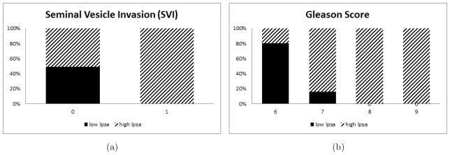
Distributions of the subgroups discovered by the proposed method in the Prostate dataset for the categorical variables SVI and Gleason score. Note that the circle subgroup (higher lpsa) mostly comprises the higher end of the Gleason score and comprises the presence for SVI entirely.

10 Discussion

In this paper, a new type of machine learning task was introduced called latent supervised learning. This type of learning represents a paradigm shift away from the conventional assumption that labels are either completely unavailable (as in unsupervised learning) or when available, hard-coded truths (as in supervised learning) to the more realistic idea that labels are actually “fuzzy” in nature. A specific problem in latent supervised learning was studied called the change-line classification problem. The proposed estimator was shown to be accurate on simulated data and provide meaningful and interpretable results on real datasets.

A major challenge to the proposed methodology is high dimensional data settings. The simulations in Section 8 show that the performance of the proposed method suffers when dimension is increased from 5 to 25. The high dimensional setting presents various challenges already familiar to modern statisticians. If sparsity is assumed for the coefficients of the normal vector to the separating hyperplane, likelihood penalization is a promising approach. This is an active field of research and many existing techniques can be borrowed for extending the proposed method to high dimensional settings. Another approach is to improve the construction of the simple sieve. This currently requires training a binary linear classifier given a particular enumeration of the class labels. When the dimension is very high, noise will hamper the accuracy of the candidate directions in the simple sieve. The boosting in the second part of the sieve construction may not be enough to compensate for the effects of the noise. A simple solution is to first reduce the dimension of the covariates using principal component analysis. Directions along which there is very little variation are unlikely to play an important role in the classification rule and thus can be safely discarded.

Other future problems include extending Model (1) to the case where Y is a survival time. It is of direct clinical interest to find subgroups that are homogeneous with respect to some biological characteristic, gene expression for example, but differ with respect to survival. The extension to survival data would be straightforward if the survival times were completely observed but will require careful development in the case of censoring. Work has begun to address the case of right-censored survival data.

Another problem of interest is to extend the change-line classification problem studied here to the change-line regression problem. In the regression problem, the regression function changes when crossing a separating hyperplane in the covariate space. This could be of interest to fields like personalized medicine which postulate that different subgroups experience different treatment effects.

As for the theoretical aspects of the proposed methodology, rate of convergence and weak convergence of the estimator remain open problems. A closer look at the simple sieve defined in Section 5.2 and Lemma 3 reveals that the simple sieve is much richer than necessary. However despite this, it does not perform nearly as well as the boosted sieve as evidenced by simulations in Section 8. This suggests that boosting may induce a speed-up of the rate of convergence and hence yield better performance on finite samples.

A Proofs

Lemma 1

Let ${\mathrm{\Theta }}_{K_1,K_2}:=\{\theta =({\mu }_1,{\sigma }_1^2,{\mu }_2,{\sigma }_2^2):\mid {\mu }_1\mid ,\mid {\mu }_2\mid <K_1,\frac{1}{K_2}<{\sigma }_1^2,{\sigma }_2^2<K_2\}$ where K₁ ∈ (0, ∞) and K₂ ∈ (1, ∞). Let (X₁, Y₁), …, (X_n, Y_n) be iid from Model (1), under Assumptions (A1) – (A6), the class of functions

$$\{m_{\omega ,\gamma ,\theta }(x,y):(\omega ,\gamma )\in {\mathbb{S}}^d\times [a,b],\theta \in {\mathrm{\Theta }}_{K_1,K_2}\}$$

is Glivenko-Cantelli.

Proof of Lemma 1

Recall the definition of m:

$$m_{\omega ,\gamma ,\theta }(x,y)=-log[({\sigma }_1^2-{\sigma }_2^2)1\{{\omega }^{T}x-\gamma \ge 0\}+{\sigma }_2^2]-\frac{{[y-({\mu }_1-{\mu }_2)1\{{\omega }^{T}x-\gamma \ge 0\}-{\mu }_2]}^2}{({\sigma }_1^2-{\sigma }_2^2)1\{{\omega }^{T}x-\gamma \ge 0\}+{\sigma }_2^2}$$

Lemma 8.12 in Kosorok (2008) establishes the measurability of the class of indicator functions {1(ω^T x − γ ≥ 0): (ω, γ) ∈ K}. Standard Vapnik-Chervonenkis (VC) class arguments then show the class {1(ω^T x − γ ≥ 0): (ω, γ) ∈ K} is Glivenko-Cantelli. The classes

$$\{{\mu }_j:(\omega ,\gamma )\in {\mathbb{S}}^d\times [a,b],\theta \in {\mathrm{\Theta }}_{K_1,K_2}\}$$

and

$$\{{\sigma }_j^2:(\omega ,\gamma )\in {\mathbb{S}}^d\times [a,b],\theta \in {\mathrm{\Theta }}_{K_1,K_2}\}$$

for j = 1, 2 are trivially Glivenko-Cantelli as they are not data-dependent. Furthermore, these classes have integrable (in fact finite) envelopes by the definition of Θ_K1,K2. The preservation result given by Corollary 9.27 (i) and (ii) in Kosorok (2008) can now be applied to show the classes

$$\begin{array}{cc}\{({\mu }_1-{\mu }_2)1\{{\omega }^{T}x-\gamma \ge 0\}+{\mu }_2\}& \text{with}\text{envelope}{K}_1,\\ \{({\sigma }_1^2-{\sigma }_2^2)1\{{\omega }^{T}x-\gamma \ge 0\}+{\sigma }_2^2\}& \text{with}\text{envelope}{K}_2,\end{array}$$

and

$$\begin{array}{cc}\{\frac{1}{({\sigma }_1^2-{\sigma }_2^2)1\{{\omega }^{T}x-\gamma \ge 0\}+{\sigma }_2^2}\}& \text{with}\text{envelope}{K}_2,\end{array}$$

are Glivenko-Cantelli with finite envelopes. Using Corollary 9.27 (iii), we have the class

$$\{log(({\sigma }_1^2-{\sigma }_2^2)1\{{\omega }^{T}x-\gamma \ge 0\}+{\sigma }_2^2)\}.$$

is Glivenko-Cantelli with integrable envelope log K₂. The class

$$\{y:(\omega ,\gamma )\in {\mathbb{S}}^d\times [a,b],\theta \in {\mathrm{\Theta }}_{K_1,K_2}\}$$

is Glivenko-Cantelli simply by the regular Law of Large Numbers. The function |y| is an envelope for this class and is integrable since E|Y| < ∞ by (A4). The class

$$\{{(y-({\mu }_1-{\mu }_2)1\{{\omega }^{T}x-\gamma \ge 0\}-{\mu }_2)}^2\}$$

has an integrable envelope since EY² < ∞ by (A4). Using Corollary 9.27 (i) and (iii), we can show the class is Glivenko-Cantelli. Applying Corollary 9.27 (i) and (ii) one last time gives the desired result that m_{ω, γ, θ} is itself a Glivenko-Cantelli class.

Lemma 2

Let (X₁, Y₁), …, (X_n, Y_n) be iid from Model (1). Under Assumptions (A1)–(A6), the class of functions

$$\{m_{\omega ,\gamma ,\theta (\omega ,\gamma )}:(\omega ,\gamma )\in {\mathbb{S}}^d\times [a,b]\}$$

is Glivenko-Cantelli.

Proof of Lemma 2

We can apply Lemma 1 directly to show the desired result. First we show there exists some K₁ ∈ [0, ∞) such that |μ₁(ω, γ)|, |μ₂(ω, γ)| < K₁ for all (ω, γ) ∈ × [a, b]. For the class of functions {μ₁(ω, γ)}, we can write

$$\begin{array}{l}{\mu }_1(\omega ,\gamma )=\frac{P(Y1\{{\omega }^{T}X-\gamma \ge 0\})}{P(1\{{\omega }^{T}X-\gamma \ge 0\}}\\ =\frac{1}{P(1\{{\omega }^{T}X-\gamma \ge 0\}}P(\{Y1\{{\omega }_0^{T}X-{\gamma }_0\ge 0\}+Y1\{{\omega }_0^{T}X-{\gamma }_0\ge 0\}\}1\{{\omega }^{T}X-\gamma \ge 0\})\\ =\frac{1}{P(1\{{\omega }^{T}X-\gamma \ge 0\}}P(\{{\mu }_{1,0}1\{{\omega }_0^{T}X-{\gamma }_0\ge 0\}+{\mu }_{2,0}1\{{\omega }_0^{T}X-{\gamma }_0\ge 0\}\}1\{{\omega }^{T}X-\gamma \ge 0\})\\ \le max{\mu }_{1,0},{\mu }_{2,0}\end{array}$$

The above also shows μ₁(ω, γ) ≥ min μ_1,0, μ_2,0 and thus |μ₁(ω, γ)| ≤ K₁ = max |μ_1,0|, |μ_2,0|. Similarly, we can show |μ₂(ω, γ)| ≤ K₁.

Next we show there exists some K₂ ∈ (0, ∞) such that $\frac{1}{K_2}<{\sigma }_1^2(\omega ,\gamma ),{\sigma }_2^2(\omega ,\gamma )<K_2$. We have

$$\begin{array}{l}{\sigma }_1^2(\omega ,\gamma )=\frac{P\{{(Y-{\mu }_1(\omega ,\gamma ))}^{2}1\{{\omega }^{T}X-\gamma \ge 0\}\}}{P(1\{{\omega }^{T}X-\gamma \ge 0\}}\\ =\frac{P\{{(Y-{\mu }_1(\omega ,\gamma ))}^{2}1\{{\omega }^{T}X-\gamma \ge 0\}\{1\{{\omega }_0^{T}X-{\gamma }_0\ge 0\}+1\{{\omega }_0^{T}X-{\gamma }_0<0\}\}\}}{P(1\{{\omega }^{T}X-\gamma \ge 0\}}\\ =\frac{P\{({\sigma }_{1,0}^2+{({\mu }_{1,0}-{\mu }_1(\omega ,\gamma ))}^2)1\{{\omega }_0^{T}X-{\gamma }_0\ge 0\}1\{{\omega }^{T}X-\gamma \ge 0\}\}}{P(1\{{\omega }^{T}X-\gamma \ge 0\}}+\frac{P\{({\sigma }_{2,0}^2+{({\mu }_{2,0}-{\mu }_2(\omega ,\gamma ))}^2)1\{{\omega }_0^{T}X-{\gamma }_0<0\}1\{{\omega }^{T}X-\gamma \ge 0\}\}}{P(1\{{\omega }^{T}X-\gamma \ge 0\}}.\end{array}$$

Thus we have $c_1\le {\sigma }_1^2(\omega ,\gamma )\le c_2$ where

$$c_1=\underset{\omega ,\gamma \in K}{inf}min\{{\sigma }_{1,0}^2+{({\mu }_{1,0}-{\mu }_1(\omega ,\gamma ))}^2,{\sigma }_{2,0}^2+{({\mu }_{2,0}-{\mu }_1(\omega ,\gamma ))}^2\}$$

and

$$c_2=\underset{\omega ,\gamma \in K}{sup}max\{{\sigma }_{1,0}^2+{({\mu }_{1,0}-{\mu }_1(\omega ,\gamma ))}^2,{\sigma }_{2,0}^2+{({\mu }_{2,0}-{\mu }_1(\omega ,\gamma ))}^2\}$$

Because |μ₁(ω, γ) is bounded, we have that c₁ and c₂ are both finite. Let K₂ be such that 1/K₂ < c₁ and K₂ < c₂. Then $\frac{1}{K_2}<{\sigma }_1^2(\omega ,\gamma )<K_2$. A similar argument can be applied to ${\sigma }_2^2(\omega ,\gamma )$.

Lemma 3

Let (X₁, Y₁), …, (X_n, Y_n) be iid from Model (1). Under (A1–A6), there exists a sequence ω_n in Ω̂_n that converges to ω₀, where Ω̂_n is the boosted sieve defined in Equation (8). Further the corresponding intercept estimate γ_n ∈ [a, b] is consistent for γ₀.

Proof of Lemma 3

Recall that the sieve Ω̂_n is populated by boosted MD directions

$$\{{\widehat{\nu }}_n{({\omega }^{MD}(P),{\gamma }^{MD}(P))}^T{\widehat{\mathrm{\sum }}}_{xx}^{-1/2}:P\in \underset{k}{\cup }{\mathcal{P}}_k\}$$

where ν̂_n is the largest eigenvector of V̂_n which was defined in Equation (7) as

$${\widehat{V}}_n(\omega ,\gamma )=\sum _{h=1}^H(\mid I_{h,1}(\omega ,\gamma )\mid {\widehat{m}}_{h,1}(\omega ,\gamma ){\widehat{m}}_{h,1}{(\omega ,\gamma )}^{\prime }+\mid I_{h,2}(\omega ,\gamma )\mid {\widehat{m}}_{h,2}(\omega ,\gamma ){\widehat{m}}_{h,2}{(\omega ,\gamma )}^{\prime }).$$

Let p_h,1(ω, γ) = E1{Y ∈ I_h, ω^TX − γ ≥ 0} and p_h,2(ω, γ) = E1{y ∈ I_h, ω^TX − γ < 0} be the theoretical proportions in each sub-slice. Let $Z={\mathrm{\sum }}_{xx}^{-1}[X-EX]$ be the standardized co-variate and m_h,1(ω, γ) = E[E(Z|Y )|Y ∈ I_h, ω^TX − γ ≥ 0] and m_h,2(ω, γ) = E[E(Z|Y )|Y ∈ I_h, ω^TX − γ < 0] be the theoretical means in each sub-slice. Define the matrix

$$V(\omega ,\gamma )=\sum _{h=1}^H{p}_{h,1}(\omega ,\gamma )m_{h,1}{m}_{h,1}{(\omega ,\gamma )}^{\prime }+\sum _{h=1}^H{p}_{h,2}(\omega ,\gamma )m_{h,2}(\omega ,\gamma )m_{h,2}{(\omega ,\gamma )}^{\prime }.$$

It is easy to see V̂_n(ω, γ) is uniformly consistent for V (ω, γ) over (ω, γ) ∈ × [a, b]. By Corollary 3.1 in Li (1991) which uses (A5), the largest eigenvector of V (ω, γ) falls in the linear space generated by ${\omega }_0{\mathrm{\sum }}_{xx}^{1/2}$. Since ν̂_n(ω, γ) is consistent for the largest eigenvector of V(ω, γ) and Σ̂_xx is consistent for Σ_xx, we have ${\widehat{\nu }}_n{(\omega ,\gamma )}^T{\widehat{\mathrm{\sum }}}_{xx}^{-1/2}\to {\omega }_0$ uniformly over (ω, γ) ∈ × [a, b]. We can find a corresponding intercept estimate that is consistent in the following manner. For a consistent estimator ω_n of ω₀, the corresponding intercept estimate given by

$$\begin{array}{l}{\gamma }_n=min\underset{\gamma \in {\widehat{\mathrm{\Gamma }}}_n({\omega }_n)}{argmax}{L}_n({\omega }_n,\gamma ,{\widehat{\theta }}_n({\omega }_n,\gamma ))\\ =min\underset{\gamma \in {\widehat{\mathrm{\Gamma }}}_n({\omega }_n)}{argmax}{M}_n({\omega }_n,\gamma ,{\widehat{\theta }}_n({\omega }_n,\gamma ))\end{array}$$

is consistent for γ₀. To see this, we invoke the Argmax Theorem in Kosorok (2008) along with the continuity of M to show γ_n converges to the argmax over γ of M (ω₀, γ, θ(ω₀, γ). By the proof in Theorem 1 however, the argmax of M(ω₀, γ, θ(ω₀, γ)) over γ is γ₀.

Lemma 4

Let M_n and θ̂_n be as defined in Section 6 and Equation (5), respectively. Under Assumptions (A1–A6), we have

$$\underset{(\omega ,\gamma )\in {\mathbb{S}}^d\times [a,b]}{sup}\mid M_n(\omega ,\gamma ,{\widehat{\theta }}_n(\omega ,\gamma ))-M_n(\omega ,\gamma ,\theta (\omega ,\gamma ))\mid \to 0$$ (13)

in probability.

Proof

In general, if a class of functions is GC then |P_nf − Pf| → 0 in probability uniformly in f varying over . It is obvious then that |P_nf̂_n − Pf̂_n| → 0 in probability for every sequence of random functions f̂_n contained in . Furthermore if f̂_n → f₀ and the random sequence is dominated so that Pf̂_n → Pf₀ then it follows that P_nf̂_n → Pf₀.

In Lemma 2, it was shown that for some K₁, K₂, θ(ω, γ) ∈ Θ_K1,K2 for all (ω, γ) ∈ × [a, b]. It follows that there exists a δ-neighborhood around θ( ω, γ) that lives in ${\mathrm{\Theta }}_{K_1^{\prime },K_2^{\prime }}$ for some $K_1^{\prime },K_2^{\prime }$ for all (ω, γ) ∈ × [a, b]. To see this, set $K_1^{\prime }=K_1+\delta$ and let $K_2^{\prime }$ be such that $K_2+\delta <K_2^{\prime }$ and $1/K_2^{\prime }<1/K_2-\delta$. Thus the enlarged class

$${\mathcal{F}}^{\delta }=\{m_{\omega ,\gamma ,\theta }(x,y):(\omega ,\gamma )\in {\mathbb{S}}^d\times [a,b],\theta \in {\theta }^{\delta }(\omega ,\gamma )\}$$

is contained in ${\mathrm{\Theta }}_{K_1^{\prime },K_2^{\prime }}$ and is hence GC. By Lemma 5, θ̂_n is uniformly consistent for θ over (ω, γ) ∈ × [a, b]. Then we have θ̂_n(ω, γ) ∈ θ^δ(ω, γ) for n large enough for all (ω, γ) ∈ × [a, b]. This implies the class of functions

$$\{m_{\omega ,\gamma ,{\widehat{\theta }}_n(\omega ,\gamma )}(x,y):(\omega ,\gamma )\in {\mathbb{S}}^d\times [a,b]\}\subset {\mathcal{F}}^{\delta }$$

for n large enough and is hence Glivenko-Cantelli, i.e.

$$\underset{(\omega ,\gamma )\in {\mathbb{S}}^d\times [a,b]}{sup}\mid M_n(\omega ,\gamma ,{\widehat{\theta }}_n(\omega ,\gamma ))-M(\omega ,\gamma ,{\widehat{\theta }}_n(\omega ,\gamma ))\mid \to 0$$

in probability. Then we have by the continuity of M,

$$\underset{(\omega ,\gamma )\in {\mathbb{S}}^d\times [a,b]}{sup}\mid M_n(\omega ,\gamma ,{\widehat{\theta }}_n(\omega ,\gamma ))-M(\omega ,\gamma ,\theta (\omega ,\gamma ))\mid \to 0$$

in probability. Using this and Lemma 2 once again, we have

$$\begin{array}{l}\underset{(\omega ,\gamma )\in {\mathbb{S}}^d\times [a,b]}{sup}\mid M_n(\omega ,\gamma ,{\widehat{\theta }}_n(\omega ,\gamma ))-M_n(\omega ,\gamma ,\theta (\omega ,\gamma ))\mid \\ \le \underset{(\omega ,\gamma )\in {\mathbb{S}}^d\times [a,b]}{sup}\mid M_n(\omega ,\gamma ,{\widehat{\theta }}_n(\omega ,\gamma ))-M(\omega ,\gamma ,\theta (\omega ,\gamma ))\mid \\ +\underset{(\omega ,\gamma )\in {\mathbb{S}}^d\times [a,b]}{sup}\mid M_n(\omega ,\gamma ,\theta (\omega ,\gamma ))-M(\omega ,\gamma ,\theta (\omega ,\gamma ))\mid \\ =o_P(1)+o_P(1).\end{array}$$

Thus we have proven (13).

Lemma 5

Let θ̂_n be as defined in Equation (5). Under Assumptions (A1–A6), θ̂_n(ω, γ) is uniformly consistent for θ( ω, γ) over (ω, γ) ∈ × [a, b], i.e.

$$\underset{(\omega ,\gamma )\in {\mathbb{S}}^d\times [a,b]}{sup}\mid {\widehat{\theta }}_n(\omega ,\gamma )-\theta (\omega ,\gamma )\mid \to 0$$

in probability.

Proof

We showed in Lemma 1 the classes {y: (ω, γ) ∈ × [a, b], θ ∈ Θ_K1,K2} is Glivenko Cantelli with an integrable envelope. We also showed the class of indicator functions 1{ω^T X − γ ≥ 0} is Glivenko-Cantelli. We can apply Corollary 9.27 (ii) in Kosorok (2008) to see the numerator of μ̂₁, $n^{-1}{\sum }_{i=1}^n{y}_{i}1\{{\omega }^T{x}_i-\gamma \ge 0\}$, converges in probability to P (Y 1{ω^T X − γ ≥ 0}) uniformly over (ω, γ) ∈ × [a, b]. The denominator $n^{-1}{\sum }_{i=1}^{n}1\{{\omega }^T{x}_i-\gamma \ge 0\}$ converges in probability to P (1{ω^TX − γ ≥ 0}) which is bounded away from zero, uniformly over (ω, γ) ∈ × [a, b]. Thus μ̂₁(ω, γ) converges in probability to μ₁(ω, γ) uniformly. A similar argument can be applied to μ̂₂(ω, γ).

The estimated variance ${\widehat{\sigma }}_1^2$ is given by

$${\widehat{\sigma }}_1^2(\omega ,\gamma )=\frac{{\sum }_i{(y_i-{\widehat{\mu }}_1(\omega ,\gamma ))}^{2}1\{{\omega }^T{x}_i-\gamma \ge 0\}}{{\sum }_{i}1\{{\omega }^T{x}_i-\gamma \ge 0\}}.$$

The numerator converges to P ((Y − μ₁(ω, γ))²1{ω^TX − γ ≥ 0}) while the denominator converges to P (1{ω^T X − γ ≥ 0}) which is bounded away from zero by assumption. Thus ${\widehat{\sigma }}_1^2(\omega ,\gamma )$ converges in probability to ${\sigma }_1^2(\omega ,\gamma )$ uniformly over (ω, γ) ∈ × [a, b]. A similar argument can be applied to ${\widehat{\sigma }}_2^2(\omega ,\gamma )$.

B Data pre-processing and summary of data features

The Cleveland Heart Disease Dataset is available at the UCI Machine Learning Repository (Frank and Asuncion, 2010). The dataset actually contains 76 features but most published work seem to focus on the subset listed in Table 7. There is a feature titled “goal”, valued from 0 to 4, corresponding to the degree of heart disease in the patient. The presence of heart disease (1,2,3,4) was combined into a single group versus the absence of heart disease (0).

The Pima Indian Diabetes Dataset is also available at the UCI machine learning repository. The binary variable of interest is whether the patient has diabetes. The dataset also contains information on various clinical measurements, summarized in Table 7. This is a large dataset with 768 cases. Some minimal preprocessing was necessary as certain cases have missing values encoded by 0 (where a 0 value would actually be biologically impossible). 3-Nearest Neighbors was used to impute the missing values. Also, a large number of cases (about 300) are missing feature 5, the two hour serum insulin measurement, which was taken to be the surrogate variable.

The Prostate Cancer dataset was analyzed in Chapter 1 of Hastie et al. (2003) and is available on the authors’ website. No preprocessing was necessary.

Table 7.

Dataset Features

Heart	Diabetes	Prostate
age in years 1= male, 0 = female chest pain type resting blood pressure serum cholesterol fasting blood sugar indicator resting electrocardiographic results maximum heart rate achieved exercise induced angina indicator ST depression induced by exercise relative to rest slope of the peak exercise ST segment number of major vessels colored by fluoroscopy 3 = normal, 6 = fixed defect, 7 = reversable defect	Number of times pregnant Plasma glucose concentration Diastolic blood pressure Triceps skin fold thickness Body mass index Diabetes pedigree function Age (years)	log cancer volume (lcavol) log prostate weight (lweight) age log of the amount of benign prostatic hyperplasia (lbph) seminal vesicle invasion (svi) log of capsular penetration (lcp) Gleason score (gleason) percent of Gleason scores 4 or 5 (pgg45)

References

- Carlstein E, Müller H, Siegmund D. Number v. 23 in Lecture notes-monograph series. Institute of Mathematical Statistics; 1994. Change-Point Problems. [Google Scholar]
- Fleming TR. Surrogate Endpoints And FDA’s Accelerated Approval Process. Health A3. 2005;24(1):67–78. doi: 10.1377/hlthaff.24.1.67. [DOI] [PubMed] [Google Scholar]
- Frank A, Asuncion A. UCI machine learning repository. 2010. [Google Scholar]
- Geman S, Hwang CR. Nonparametric Maximum Likelihood Estimation by the Method of Sieves. The Annals of Statistics. 1982;10(2):401–414. [Google Scholar]
- Grenander U. Abstract Inference. Wiley; 1981. [Google Scholar]
- Hastie T, Tibshirani R, Friedman JH. The Elements of Statistical Learning. Springer; 2003. corrected edition. [Google Scholar]
- Jain AK, Murty MN, Flynn PJ. Data clustering: a review. ACM Comput Surv. 1999;31(3):264–323. [Google Scholar]
- Kang C. PhD thesis. UNC; Chapel Hill: 2011. New Statistical Learning Methods for Chemical Toxicity Data Analysis. [Google Scholar]
- Kosorok MR. Introduction to Empirical Processes and Semiparametric Inference (Springer Series in Statistics) 1 Springer; 2008. [Google Scholar]
- Li KC. Sliced inverse regression for dimension reduction. Journal of the American Statistical Association. 1991;86(414):316–327. [Google Scholar]
- MSL, GSF, PMO, FJP, CES, THM Impaired chronotropic response to exercise stress testing as a predictor of mortality. JAMA: The Journal of the American Medical Association. 1999;281(6):524–529. doi: 10.1001/jama.281.6.524. [DOI] [PubMed] [Google Scholar]
- Scholkopf B, Smola AJ. Learning with Kernels: Support Vector Machines, Regularization, Optimization, and Beyond. MIT Press; Cambridge, MA, USA: 2001. [Google Scholar]
- Shen X, Shi J, Wong WH. Random sieve likelihood and general regression models. Journal of the American Statistical Association. 1999;94(447) [Google Scholar]
- Tibshirani R, Hastie T, Narasimhan B, Chu G. Diagnosis of multiple cancer types by shrunken centroids of gene expression. Proceedings of the National Academy of Sciences. 2002;99(10):6567–6572. doi: 10.1073/pnas.082099299. [DOI] [PMC free article] [PubMed] [Google Scholar]