Likelihood Formulation of Parent-of-Origin Effects on Segregation Analysis, Including Ascertainment

Abstract

We developed a likelihood-based method for testing for parent-of-origin effect in complex diseases. The likelihood formulations model parent-of-origin effect and allow for incorporation of ascertainment, as well as differential male and female ascertainment probabilities. The results based on simulated data indicated that the estimates of parental effect (either maternal or paternal) were biased when ascertainment was ignored or when the wrong ascertainment model was used. The exception was single ascertainment, in which we proved that ignoring ascertainment does not bias the estimation of parental effect, in a simple parent-of-origin model. These results underscore the importance of considering ascertainment models when testing for parent-of-origin effect in complex diseases.

Introduction

Parent-of-origin effect refers to differential penetrance or expression of disease in the offspring, depending on the sex of the transmitting parent. Parent-of-origin effect may encompass several possible underlying biological phenomena, including genomic imprinting, trinucleotide-repeat expansion, or mitochondrial inheritance. Genomic imprinting (also referred to as “gametic” or “parental” imprinting) is the epigenetic marking of a gene, on the basis of its parental origin, that results in monoallelic expression. Genomic imprinting differs from classical Mendelian genetics in that the parental complements of imprinted genes are not equivalent with respect to their expression. In maternal imprinting, gene expression is inhibited after passage through the mother’s germline, whereas, in paternal imprinting, gene expression is inhibited after passage through the father’s germline. Prader-Willi syndrome (maternally imprinted) and Angelman syndrome (paternally imprinted) are two classic examples of the numerous human diseases in which the effects of imprinting are observed (Falls et al. 1999). Studies have revealed that genomic imprinting has the following intrinsic properties: silencing of gene expression, stable propagation in dividing somatic cells, possible reversal of the imprint pattern under certain conditions, and establishment of the imprint during gametogenesis. The mechanism(s) of genomic imprinting are complex and not well understood; however, evidence suggests that methylation is a likely candidate, since it satisfies the aforementioned criteria (Tycko et al. 1997; Constancia et al. 1998).

Another biological phenomenon that can result in a parent-of-origin effect is trinucleotide-repeat expansion. Instability in expansion of trinucleotide repeats (e.g., CAG, CGG, CTG, and GAA) is observed during germline transmission when the length of the repeat exceeds a critical value (Reddy and Housman 1997). The instability is generally observed when the transmitted repeat size is 40–100 bp. Studies of individuals diagnosed with early-onset Huntington disease have revealed a significant increase in sperm trinucleotide repeat (CAG) lengths compared with the repeat lengths of the father. On the other hand, in Fragile X syndrome, expansion of trinucleotide repeats (CGG) in the FMR1 gene is observed when the gene is transmitted maternally. Numerous models have been proposed to explain the triplet-repeat expansion leading to human disease (Pearson and Sinden 1998). For example, one model involves the formation of DNA hairpin structures that lead to errors in replication (e.g., replication slippage) and/or promote recombination via unequal sister-chromatid exchange.

A third phenomenon is mitochondrial inheritance, which manifests a transmission pattern consistent with parent-of-origin effect. mtDNA is almost exclusively maternally inherited (Lightowlers et al. 1997), but a mitochondrial disorder may exhibit either a maternal or a Mendelian inheritance pattern, depending on the site of the primary gene defect. Leber hereditary optic neuropathy was the first disease found to be caused by a point mutation in mtDNA (Wallace et al. 1988); since then, numerous other mutations that lead to diseases such as myoclonic epilepsy and ragged-red fibers, mitochondrial encephalomyopathy, lactic acidosis and stroke-like episodes, and progressive external ophthalmoplegia have been found. The clinical spectrum of possible mitochondrial defects has been expanded to include several common disorders. In disorders such as Parkinson disease and Alzheimer disease, mitochondrial defects may not be the primary cause but have been suggested to modify the outcome of disease (Suomalainen 1997).

The phenomenon of parent-of-origin effect has been investigated in the transmission of neurological and psychiatric diseases such as Tourette syndrome, bipolar disorder, and panic disorder (Lichter et al. 1995; McMahon et al. 1995; Stine et al. 1995; Gershon et al. 1996; Kato et al. 1996; Eapen et al. 1997; Battaglia et al. 1999; Haghighi et al. 1999). In previous studies, similar approaches have been adopted in the analysis of disease transmission. Some investigators have systematically ascertained two-generation pedigrees and have dichotomized their data into maternal- and paternal-transmission groups (McMahon et al. 1995). Others have utilized multigenerational pedigrees and have divided them into maternal- and paternal-transmission branches (Gershon et al. 1996; Haghighi et al. 1999). The latter approach discards valuable information by breaking down multigenerational pedigrees into maternal and paternal branches and by ignoring parental mating types (MTs) in which maternal or paternal transmission cannot be determined (i.e., unaffected × unaffected and affected × affected MTs). In the consideration of the maternal and paternal branches, these methods do not account for the potential transmission of the disease gene through the unaffected parent (via reduced penetrance). Also, these methods do not incorporate ascertainment models. Consequently, we developed a likelihood-based approach that utilizes all available data for testing for parent-of-origin effect, allowing for modeling of ascertainment (Haghighi and Hodge 1999).

The likelihood-based method presented here models parent-of-origin effect in nuclear families, for a single locus. Extension of this model to general pedigree structures is described in the “Discussion” section. The likelihood calculation handles all possible parental MTs and variable sibship sizes. For each family in the data set, the exact likelihood is computed, allowing for reduced penetrance. This entails consideration of possible disease-gene transmission from unaffected parent(s) to offspring who, in turn, may or may not express the disease phenotype. The likelihood is parameterized to model parental effect, by including the penetrances of maternal and paternal transmission. To assess the potential effect that ascertainment has on detection of parent-of-origin effect or on estimation of penetrances of maternal and paternal transmission, we also incorporated a general ascertainment model into our likelihood formulation. We demonstrated that, in the special case of single ascertainment, no correction needs to be made for ascertainment (for this simple model).

The two goals of this paper are (1) to formulate the correct full likelihood for parent-of-origin effect in nuclear families, incorporating the “π”-based ascertainment model of Weinberg (1928) and Morton (1959) but also allowing for differential male and female ascertainment probabilities, and (2) to determine the effects that ascertainment has on our ability to detect parent-of-origin effect. We demonstrate the likelihood derivation and assess its utility, using simulated data generated under a range of inheritance and ascertainment models. The two principal likelihood models that are presented consist of the parental-effect model and the parental-effect-with-ascertainment model. These models were systematically studied by using simulated data generated under maternal or paternal parental effects with “complete” or “single” ascertainment. The likelihood models were evaluated by examining the estimated parental effect and the power to detect such an effect in the presence or absence of ascertainment.

Methods

Notation

To test for parent-of-origin effect, we have developed two likelihood models. Model I models parent-of-origin effect but does not incorporate ascertainment. This model would apply to situations of “random” ascertainment (see the “Discussion” section). Model II models parent-of-origin effect and also incorporates ascertainment, as well as allowing for differential male and female ascertainment probabilities. Before describing the models in detail, we will define the parameters used in the likelihood formulations:

• q=frequency of disease allele (denoted by “D”);

• p=frequency of nondisease allele (denoted by “d”), where p=1-q;

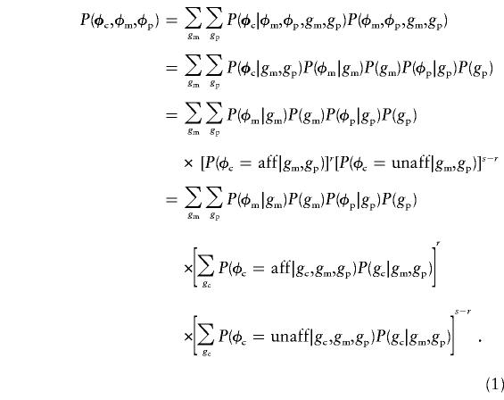
• f=diseasepenetrance, defined as the mean between the maternal- and paternal-transmission penetrances, f=(f_m+f_p)/2 (see below);

• δ=deviation of the maternal- and paternal-transmission penetrances from the mean penetrance, where δ may be either positive or negative—that is, δ=(f_m+f_p)/2 so that

  • f_m=maternal-transmission penetrance, defined as f+δ;

  • f_p=paternal-transmission penetrance, defined as f-δ;

  • f_mp=f_m+f_p-f_mf_p;

•  (note that explanations for each of these penetrance probabilities are given in the subsection “Likelihood Model I,” below);

• π_b=male ascertainment probability—that is, P(male is a proband|he is affected);

• π_g=female ascertainment probability—that is, P(female is a proband|she is affected);

• s_b=number of male offspring in a sibship;

• s_g=number of female offspring in a sibship;

• s=sibshipsize, defined as s=s_b+s_g;

• r_b=number of affected male offspring;

• r_g=number of affected female offspring;

• r=number of affected offspring, defined as r=r_b+r_g.

Note that “b” (for “boy”) and “g” (for “girl”) are used to denote male and female offspring, respectively. Also, in both likelihood models, I and II, δ is the parameter of interest; it is a nongenetic (i.e., “dummy”) parameter, which is used as an indicator of maternal or paternal transmission. The use of δ in this manner reduces model complexity, since the maternal- and the paternal-transmission penetrances are both defined with respect to one parameter (see the “Discussion” section).

Likelihood Model I

We began by calculating the exact likelihood for each of the four phenotypic parental MTs: (1) affected mother × unaffected father, (2) unaffected mother × affected father, (3) unaffected mother × unaffected father, and (4) affected mother × affected father. We assumed an autosomal dominant mode of inheritance. For each phenotypic MT, we enumerated the possible underlying parental genotypes consistent with the genetic model. These parental genotypes were then used to enumerate the possible offspring genotypes and to assign probabilities to them (see equation (1), below). A sample likelihood computation for the unaffected mother × unaffected father MT is shown in table 1, with corresponding parental probabilities, as well as offspring penetrance and transmission probabilities. We chose to illustrate this particular MT because it illustrates the use of all possible underlying parental genotypes. The remaining parental MTs are calculated in the same fashion, except that, depending on the parental phenotypes, not all parental genotypes are possible. Thus, the likelihood tables for these other MTs will contain some empty cells.

Table 1.

Transmission Probabilities (of Offspring Genotypes) and Penetrances (of Offspring Phenotypes), Conditioned on Indicated Parental Genotypes, for Parental Genotypes Compatible with Unaffected Mother × Unaffected Father MT^[Note]

	Transmission Probabilities When Unaffected Mother's Genotype Is
UnaffectedFather's Genotype	dd; p2	Dd; 2pq(1-f)	DD; q2(1-f)
dd; p2	dd; P(dd)=1, P(aff|dd)=0, P(unaff|dd)=1	dd; P(dd)=.5, P(aff|dd)=0, P(unaff|dd)=1
		Dd; P(Dd)=.5, P(aff|Dd)=fm, P(unaff|Dd)=1-fm	Dd; P(Dd)=1, P(aff|Dd)=fm, P(unaff|Dd)=1-fm
Dd; 2pq(1-f)	dd; P(dd)=.5, P(aff|dd)=0, P(unaff|dd)=1	dd; P(dd)=.25, P(aff|dd)=0, P(unaff|dd)=1
	Dd; P(Dd)=.5, P(aff|Dd)=fp, P(unaff|Dd)=1-fp	Dd; P(Dd)=.5, ,	Dd; P(Dd)=.5, P(aff|Dd)=fm, P(unaff|Dd)=1-fm
		DD; P(DD)=.25, P(aff|DD)=fmp, P(unaff|DD)=1-fmp	DD; P(DD)=.5, P(aff|DD)=fmp, P(unaff|DD)=1-fmp
DD; q2(1-f)	Dd; P(Dd)=1, P(aff|Dd)=fp, P(unaff|Dd)=1-fp	Dd; P(Dd)=.5, P(aff|Dd)=fp, P(unaff|Dd)=1-fp
		DD; P(DD)=.5, P(aff|DD)=fmp, P(unaff|DD)=1-fmp	DD; P(DD)=1, P(aff|DD)=fmp, P(unaff|DD)=1-fmp

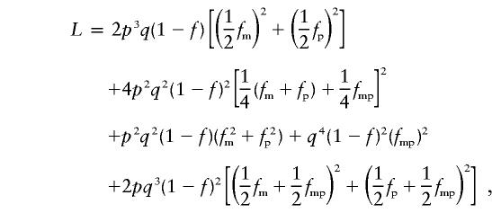
Note.— We define f_mp as f_m+f_p-f_mf_p (see text).

The exact likelihood calculation described above can be formulated as a simple probability, which is 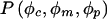, where φ_c denotes the vector (φ_c1,…,φ_cs) of the observed phenotypes of the s children, c₁,…,c_s; and φ_m and φ_p denote the observed maternal and paternal phenotypes, respectively. Using the law of total probability, we rewrite this probability to allow for all underlying genotypes, where g_m and g_p denote maternal and paternal genotypes, respectively (the symbols “φ_c” and “g_c,” not in boldface, denote the phenotype and the genotype, respectively, of a single child):

This is essentially Elston and Stewart's (1971) algorithm, except that, to model parent-of-origin effect, we condition the offspring phenotypes on the parental genotypes in addition to the usual offspring genotypes.

The probabilities in the last expression in equation (1) can be found in table 1. They are all derived from the usual functions of penetrance f and from Mendel’s first law, except the terms P(φ_c|g_c,g_m,g_p), which we now explain:

• P(φ_c=aff|g_c=dd,g_m,g_p) is assumed to be 0, independent of g_m and g_p.

• P(φ_c=aff|g_c=Dd,g_m,g_p) is taken to equal f_m (or f_p), if the Dd child clearly inherited the D allele from the mother (or father) (i.e., if one parent is Dd and the other parent is either DD or dd, or if one parent is DD and the other parent is dd). If either parent is equally likely to have contributed the D allele (i.e., if both parents are Dd), then P(φ_c=aff|g_c=Dd,g_m=Dd,g_p=Dd) is set to —that is, it is the mean of the two parental-transmission penetrances.

• For P(φ_c=aff|g_c=DD,g_m,g_p), the DD child must have received the D allele from both parents. This probability is found by first considering its complement, P(φ_c=unaff|g_c=DD,g_m,g_p). For a child with a DD genotype to be unaffected requires that the D allele not be “expressed” from either parent; thus, P(φ_c=unaff|g_c=DD,g_m,g_p)=(1-f_m)(1-f_p), under the assumption of the independence of the two parents. Therefore, P(φ_c=aff|g_c=DD,g_m,g_p)= 1-(1-f_m)(1-f_p)=f_m+f_p-f_mf_p, which we subsequently write as “f_mp” for short.

We demonstrate an actual likelihood calculation using the family in figure 1. For the sake of simplicity, we assume that the disease allele is rare (i.e., q is very small), only for this example. This reduces the likely set of parental genotypes to the following (g_m×g_p): Dd×dd and dd×Dd. (This is a simplified example; in our actual likelihood calculations, all parental genotypes are considered.) We focus on the MT Dd×dd, to illustrate the terms in equation (1). In this case, the parental penetrance terms P(φ_m|g_m) and P(φ_p|g_p) become P(φ_m=unaff|g_m=Dd)=1-f and P(φ_p=unaff|g_p=dd)=1, respectively. Similarly, the parental genotypic probabilities P(g_m) and P(g_p) become P(Dd)=2pq and P(dd)=p², respectively. The penetrance and transmission probabilities for the offspring are P(φ_c|g_c,g_m,g_p) and P(g_c|g_m,g_p), which, for the affected children, become P(φ_c=aff|g_c=Dd,g_m=Dd,g_p=dd)=f_m and P(g_c=Dd|g_m=Dd,g_p=dd) =1/2. Note that both children must have genotype Dd. The probabilities for the remaining MT are taken from table 1. Thus, the (simplified) likelihood for this family is

where the two terms correspond to the Dd×dd and dd×Dd parental mating genotypes, respectively. If we (a) did not assume that q is small and (b) included all eight possible parental genotypic MTs, the complete likelihood for this family would be,

and this is indeed what our program calculates.

Figure 1.

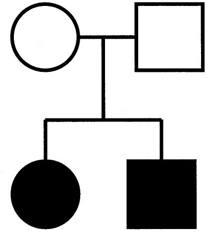
Pedigree used for illustration of likelihood calculation

Likelihood Model II

The likelihood model (i.e., model I, described above) was extended to incorporate ascertainment. This second model—model II—allows us to assess the potential influence that ascertainment has on detection of parent-of-origin effect. The potential for ascertainment bias, as is well known, is always a consideration in segregation analysis. In this case, the problem of ascertainment bias is also a concern because estimation of parental effect falls under the rubric of segregation analysis.

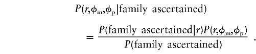
The ascertainment model assumes that families are ascertained through children (Weinberg 1928; Morton 1959) and incorporates sex-based ascertainment in the likelihood. The likelihood with differential male and female ascertainment probabilities is as follows:

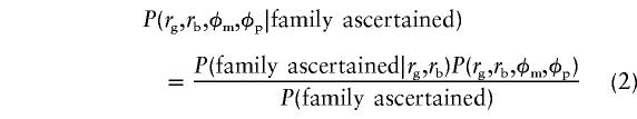Note that P(family ascertained|parental and child phenotypes) = P(family ascertained|child phenotypes), since we assume that families are ascertained through the children. Hence, the first term in the numerator of equation (2) is simply P(family ascertained|r_g,r_b). This ascertainment term, P(family ascertained|r_g,r_b), allows for modeling of general ascertainment, by a variety of possible ascertainment criteria, such as sex (male vs. female), disease subtypes (e.g., early onset vs. late onset and mild vs. severe), and so on. In this situation, we were interested in modeling the differential male and female ascertainment probabilities, so, for any π_g and π_b, this ascertainment probability for a family can be expressed as 1-(1-π_g)^r_g(1-π_b)^r_b. The second term in the numerator, P(r_g,r_p,φ_m,φ_p), corresponds to P(φ_c,φ_m,φ_p) derived in equation (1), here with r=r_g+r_b. Thus, the numerator of equation (2) becomes

The denominator of equation (2) is found by summing the numerator over all possible configurations for sibship sizes and all possible parental phenotypes:

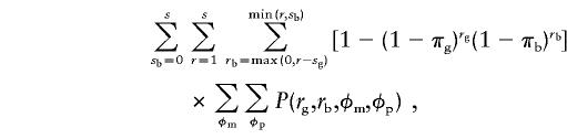where r_g=r-r_b and s_g=s-s_b. Proceeding from left to right, the first summation traverses through all sibship configurations with respect to sex; the second summation enumerates all sibship configurations with at least r=1 to, at most, r=s affected children; and the third summation keeps track of the sex of the affected children, which is used in the ascertainment term. The last two (internal) summations traverse through all possible parental phenotypes. Thus, the expanded form of equation (2) for unequal male and female ascertainment probabilities is

where each is given by equation (1).

For the special case in which the male and female ascertainment probabilities are equal (i.e., π_g=π_b=π), equation (3) is simplified, such that

In the numerator, the ascertainment term is now P(familyascertained|r)=1-(1-π)^r, and P(r,φ_m,φ_p) is as in equation (1). In the denominator, the sibship is traversed with respect to affection status but not sex. The final probability for equal male and female ascertainment probabilities becomes

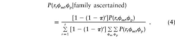Models I and II described above give the full likelihood for a single nuclear family. The likelihood for a collection of families is found by multiplying the individual family likelihoods over all families:

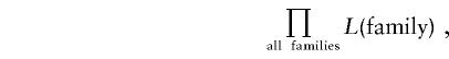where the likelihood of the individual family is given by equation (1), for model I, and by equations (3) or (4), for model II.

Details of Simulation and Analysis

We designed and implemented a simulation program (sim_poo.pl) to simulate nuclear families under the likelihood models described above. The parental MTs (i.e., both genotypes and phenotypes) were randomly generated, on the basis of Hardy-Weinberg proportions and the user-defined disease penetrances and allele frequencies. Next, offspring genotypes were generated assuming Mendelian laws of inheritance. The affection statuses of the offspring were randomly determined, given the user-defined maternal- and paternal-transmission penetrance probabilities and conditioning on offspring and parental genotypes.

We examined three situations (by “situation,” we mean a combination of generating model [GM], analysis model [AM], family structure, and data-set size).

• Situation 1. 

  Fixed family structure, rare disease (q=0.0001). Data set includes 100 families (four sibs/sibship). GM includes complete and single ascertainment; selected values of f and of δ. AM includes complete, single, and random ascertainment.

• Situation 2. 

  Variable sibship sizes. Data set includes 50 families; otherwise same as situation 1.

• Situation 3. 

  Higher gene frequency (q=0.1); otherwise, same as situation 2, except that AM includes only complete and random ascertainment.

For each situation, we evaluated some or all of the following: (a) bias in the estimate of δ, (b) power to detect parent-of-origin effect when δ>0, and (c) type I error rate when there is no parent-of-origin effect (i.e., when δ=0). To assess bias in the estimate of δ, we used the sample mean of the maximum-likelihood estimates (MLEs) of δ (henceforth denoted simply as “”). For detection of power, we used the asymptotic approximation, 2ln(LR)∼χ²(1df), where LR is the likelihood ratio of versus L(δ=0). For analysis of type I error rate (α), we set the nominal test size to 0.05 and then determined the actual test size from our simulations. Power was computed for a test size of α=0.05.

Each simulated family was then considered for inclusion in the sample, subject to a user-specified ascertainment criterion (i.e., “complete” ascertainment, single ascertainment, or “random” ascertainment). Under complete ascertainment, the family was ascertained with probability unity if there was at least one affected child in the sibship. (Thus, by “complete” ascertainment we mean the case in which π=1. This situation was originally termed “truncate” ascertainment by Morton [1959], because the corresponding probability distribution is a truncated binomial distribution; however, since many investigators currently refer to this model as “complete” ascertainment, we use that terminology in this study as well.) Under single ascertainment, the probability that any one family will be ascertained is small and is proportional to the number of affected children in the family (Morton 1959; Stene 1979; Hodge and Vieland 1996) (also see Appendix A). Under random ascertainment, all families, including those with no affected children, are ascertained with a probability of unity.

The families were then analyzed with the calc_poo.pl program, which implements the aforementioned likelihood-based algorithms. The program analyzes the data under the assumption of complete, single, or random ascertainment. It yields the logarithm of LR, ln(LR), by comparing the likelihood for a range of δ values and the likelihood of δ=0 (i.e., no parent-of-origin effect). The value is recorded for each data set, and the sample mean of these estimates is calculated over all data sets. The number of data sets considered was 500–1,000, with 50–100 families per data set. The programs sim_poo.pl and calc_poo.pl were written in PERL and are available on request.

Results

We evaluated the likelihood models by simulation analyses, in which we incrementally increased the complexity of the data to emulate “real” data sets. The results are presented for a number of GMs and AMs. The models covered a range of f and δ parameter values and ascertainment criteria (i.e., complete ascertainment, single ascertainment, and “random” ascertainment). In the likelihood calculations, complete ascertainment corresponds to π_g=π_b=1.0, whereas single ascertainment corresponds to π_g=π_b=0.01. Random ascertainment means that the likelihoods were computed under model I, which assumes that all families are equally likely to be ascertained whether they have any affected children or not. For all analyses described below, values of f and of q in the AM match those in the GM.

Situation 1.—The fixed family structure and the rare-disease (q=0.0001) model enabled us to easily confirm the simulation results analytically in any given data set. The data sets consisted of 100 families, each of which had exactly four sibs per sibship. The data were generated under complete ascertainment and then were analyzed assuming complete, single, and random ascertainment (table 2). We observed that, when the AM and GM were the same, was approximately unbiased, except when the value of f was near the defined boundary limits (0 or 1) and/or δ was small (e.g., f=0.9 and δ=0.1). However, when the data were incorrectly analyzed assuming single or random ascertainment, the values were consistently lower than they were when the correct ascertainment model had been used. The values analyzed assuming random ascertainment were approximately equal to those for single ascertainment. In addition, data were generated under single ascertainment and were analyzed assuming complete, single and random ascertainment (table 3). Similar to the previous results, was approximately unbiased when the AM matched the underlying GM. Again, the values for single and random ascertainment were virtually identical (see “Discussion” and Appendix A). However, when the data were analyzed assuming complete ascertainment the values were inflated.

Table 2.

Observed Values from Simulations of Situation 1, Generated under Complete Ascertainment

		δ
AM	f	.1	.2	.3	.4	.5
Complete ascertainment	.9	.072	…	…	…	…
	.7	.101	.193	.280	…	…
	.5	.097	.198	.300	.399	.500
Single ascertainment	.9	.066	…	…	…	…
	.7	.062	.121	.195	…	…
	.5	.049	.105	.178	.269	.432
Random ascertainment	.9	.066	…	…	…	…
	.7	.061	.121	.194	…	…
	.5	.048	.105	.177	.268	.430

Table 3.

Observed Values from Simulations of Situation 1, Generated under Single Ascertainment

		δ
AM	f	.1	.2	.3	.4	.5
Complete ascertainment	.9	.082	…	…	…	…
	.7	.160	.272	.300	…	…
	.5	.189	.316	.404	.466	.500
Single ascertainment	.9	.076	…	…	…	…
	.7	.100	.198	.280	…	…
	.5	.101	.201	.298	.400	.499
Random ascertainment	.9	.076	…	…	…	…
	.7	.100	.197	.279	…	…
	.5	.101	.200	.297	.399	.499

Situation 2.—We extended our data sets to include families with variable sibship sizes, to better emulate realistic data sets with different family configurations. Also, we chose to use data sets that contained 50 families, to evaluate the performance of the likelihood models, since this would be a reasonably attainable size for a real data set. These analyses were performed using data simulated under a rare-disease model with the same parameter values and the same ascertainment models as before (tables 4 and 5). Even with the smaller data-set size, the trends in the values were consistent with those from the first set of analyses (tables 2 and 3). Specifically, for the analyses in which the AMs were the same as the GMs, was generally unbiased. The values were either lower (table 4) or higher (table 5) than expected, when the wrong ascertainment model was used in the analysis. Again, the exception occurs for single ascertainment, in which ignoring ascertainment does not bias (see table 5, “Discussion,” and Appendix A). The values that we observed when the data were analyzed assuming single or random ascertainment were always very similar.

Table 4.

Observed Values from Simulations of Situation 2, Generated under Complete Ascertainment

		δ
AM	f	.1	.2	.3	.4	.5
Complete ascertainment	.9	.061	…	…	…	…
	.7	.095	.193	.267	…	…
	.5	.095	.196	.295	.397	.499
Single ascertainment	.9	.057	…	…	…	…
	.7	.067	.136	.206	…	…
	.5	.056	.118	.192	.289	.447
Random ascertainment	.9	.057	…	…	…	…
	.7	.064	.135	.205	…	…
	.5	.055	.118	.191	.287	.445

Table 5.

Observed Values from Simulations of Situation 2, Generated under Single Ascertainment

		δ
AM	f	.1	.2	.3	.4	.5
Complete ascertainment	.9	.073	…	…	…	…
	.7	.139	.252	.296	…	…
	.5	.160	.297	.396	.464	.500
Single ascertainment	.9	.062	…	…	…	…
	.7	.100	.198	.275	…	…
	.5	.097	.199	.297	.400	.498
Random ascertainment	.9	.069	…	…	…	…
	.7	.099	.197	.275	…	…
	.5	.096	.198	.296	.399	.498

In situation 2, we also investigated the power of the likelihood models to detect parent-of-origin effect. As expected, we observed higher power when the AM matched the true GM (fig. 2A). In contrast, when the data were generated under single ascertainment, we found that power was higher when the data were analyzed assuming complete ascertainment (fig. 2B). Again, the observed power levels for analyses under single and random ascertainment were very close. Overall, the power increased with increasing parental effect in the data set (i.e., the power increased with increasing δ), as one would expect. For these analyses, power to detect a maternal effect converged to unity for δ>0.3.

Figure 2.

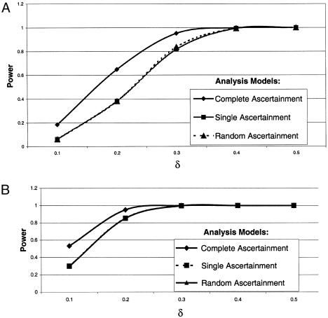
Observed power values from simulations of situation 2, for data sets generated under complete ascertainment (A) and data sets generated under single ascertainment (B). Mean f is 0.5. Note that the curves for single and random ascertainment are superimposed.

Last, for situation 2, we examined the performance of our likelihood-based methods in the absence of parent-of-origin effect, to assess type I error. In this case, the data were simulated with no parental effect (δ=0), under both complete and single ascertainment, and were analyzed assuming complete, single, and random ascertainment. For these models, the values did not appear to be influenced by potential ascertainment bias in which the resulting values were approximately equal to 0. Furthermore, for the same models, we found that the type I error rate did not exceed the nominal size of the test (0.05), except in one analysis (table 6). This exception occurred when the data were generated under single ascertainment and were analyzed assuming complete ascertainment. Note that, in the presence of a parental effect, this particular GM/AM combination always gave inflated values, yielding a higher proportion of individual data sets with inflated values, thus resulting in a higher type I error.

Table 6.

Observed Type I Error Rates from Simulations of Situation 2, in Which Nominal Test Size is 0.05

	Type I Error Rate under GM
	Complete Ascertainment			Single Ascertainment
AM Assumed	f = .9	f = .7	f = .5	f = .9	f = .7	f= .5
Complete ascertainment	.046	.045	.046	.060	.096	.144
Single ascertainment	.041	.045	.046	.041	.045	.046
Random ascertainment	.041	.045	.044	.041	.045	.044

Situation 3.—So far, all the analyses involved data generated under a rare disease model. However, our goal was to evaluate the likelihood models in the context of complex common diseases with potential parent-of-origin effect. Therefore, in situation 3 a higher disease-gene frequency (q=0.1) was used. This situation is similar to situation 2 because the data sets were generated with 50 families of variable sibship sizes under complete ascertainment and were analyzed assuming complete or random ascertainment (table 7). We found that the trends in the estimates of parental effect were the same for both the common- and rare-disease models (tables 4 and 7). However, the values were slightly lower for the common- versus the rare-disease model, for both AMs examined. This was most likely due to an increase in the proportion of uninformative parental MTs, because of the higher disease-gene frequency in the population.

Table 7.

Observed Values from Simulations of Situation 3, Generated under Complete Ascertainment

		δ
AM	f	.1	.2	.3	.4	.5
Complete ascertainment	.9	.060	…	…	…	…
	.7	.096	.190	.258	…	…
	.5	.093	.193	.288	.391	.499
Random ascertainment	.9	.056	…	…	…	…
	.7	.063	.130	.194	…	…
	.5	.050	.107	.172	.263	.407

We also performed power simulations in situation 3. For the two AMs, power to detect parental effect was consistently lower under the common-disease model. This is because, for common diseases, the proportion of informative parental MTs with distinct maternal or paternal disease-gene transmission is smaller than that for rare diseases. When the data were analyzed assuming complete ascertainment, in which the AM and GM were the same, the maximum drop in power was 22% at δ=0.2 (fig. 3A). When the same data were analyzed assuming the wrong ascertainment criterion (i.e., random ascertainment), there was a dramatic reduction in power, in which the observed drop was as high as 89% at δ=0.1 (fig. 3B). Similar to the previous observations' estimates of power for both disease models, the estimates of power increased as the magnitude of parental effect (i.e., δ) increased. Note that, for all the results presented, the data were simulated for maternal transmission (positive δs); however, when the data were generated for paternal transmission (negative δs) the results were symmetric (data not shown).

Figure 3.

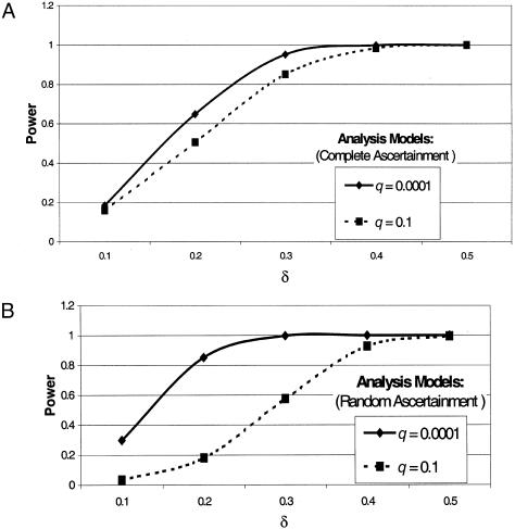
Observed power values from simulations of situation 3, for data sets generated under complete ascertainment and analyzed assuming complete ascertainment (A) and data sets generated under complete ascertainment and analyzed assuming random ascertainment (B). Mean f is 0.5.

Discussion

Summary

In this study, we first formulated likelihood-based models for parent-of-origin effect in transmission of disease, allowing for ascertainment in nuclear families. This likelihood formulation was then used to test for the existence of parent-of-origin effect and to estimate the size of this effect (δ), in the presence of different ascertainment models. Second, we evaluated the performance of the procedure under different circumstances, by means of simulation analyses. In this way, we assessed whether ascertainment bias would affect test results or estimates of δ. We showed that the estimates of δ were approximately unbiased when the data were analyzed for the same parametric GM, except when f and δ were near their defined boundary limits. The estimates of δ were biased when ascertainment was ignored or when the wrong ascertainment model was assumed. The only exception was for single ascertainment, in which the ignoring of ascertainment does not bias the estimates of δ (see below).

We examined only dominant modes of inheritance—because, in these models, the origin of the disease allele can often be determined on the basis of its maternal or paternal transmission, whereas, in recessive inheritance, both parents transmit the disease allele to the affected offspring. This may be problematic for studies of common complex diseases in which the disease gene(s) is frequent in the population, since a high proportion of the parents would be homozygous. Also, the lower the overall penetrance of the condition being studied, the more families there will be in which the transmitting parent is not phenotypically affected, so that it is not obvious whether the mother or father is the transmitting parent. An additional limitation in the model concerns our assumption of disease penetrances. The disease penetrance f is defined as the average of maternal- and paternal-transmission penetrances. In the model considered here, this average penetrance also equals the population-wide penetrance of the disease. In a more complex model (e.g., a model with differential penetrances for male and female individuals, in addition to the differential effects from male and female transmitting parents), that would no longer be the case. Also note that, in our study, the penetrance parameters are taken at a single time point and do not allow for potential age and environmental effects (e.g., drug exposure).

In our model, we assigned a disease risk of f_mp to homozygous DD children (i.e., children who have received a D allele from both parents), where f_mp is defined as f_m+f_p-f_mf_p. This definition of f_mp can be justified by a model such as the following: The child receives a “hit” from the maternal D allele with probability f_m and a hit from the paternal D allele with probability f_p; if the child receives at least one hit, then the child is affected. Dr. Gary Chase (personal communication) has pointed out that, alternatively, one could formulate a regression model such as this: let f_m and f_p represent the regression coefficients in a binary model, where Y=1 if the child is affected and Y=0 otherwise; let f_m (or f_p) represent the lifetime-risk increase associated with maternal (or paternal) transmission. Thus, our formula for f_mp represents one particular type of interaction, but other types could be modeled as well.

Importance of Ascertainment

It is well known that the ascertainment model plays a critical role in classical segregation analysis and that, except when families (i.e., including those families with no affected members) are sampled completely randomly from the population, failure to allow for ascertainment can seriously bias a segregation analysis (Morton 1959; Stene 1979; Greenberg 1986). However, it may be less obvious that the ascertainment model would also affect analyses of parent-of-origin effect. After all, in estimating δ, we are assessing not segregation ratios per se but, rather, a quantity proportional to the difference between segregation ratios. Conceivably, biases in the segregation ratios themselves would be canceled out in the difference, δ. In fact, we have demonstrated that this is what does happen when families are ascertained under single ascertainment—both in our simulations (see tables) and in a proof (see below and Appendix A). However, this does not happen for other ascertainment models. Thus, our results are important, because they indicate that, in general, it is critical to allow for ascertainment when parent-of-origin effect is being assessed.

Note that we considered only two particular ascertainment models (i.e., those for single and complete ascertainment). These correspond to special cases of more-general ascertainment models (Weinberg 1928; Morton 1959; Ewens and Shute 1986; Greenberg 1986). However, our finding that ascertainment does matter for analysis of parent-of-origin effect would presumably also hold for other cases of those ascertainment models.

We specifically considered differential ascertainment probabilities for males and females, because one can readily imagine a scenario in which females, for example, are more readily ascertained than males. This situation could arise, for example, if women are more likely to seek treatment for illnesses—in particular, psychiatric illnesses—than men are.

Our simulations (tables 3 and 5) reveal that, if data sets are generated under single ascertainment but are analyzed as if they had been randomly ascertained, then the estimates of δ appear to be unbiased. If one writes out the likelihood, L(δ), under single ascertainment, one can see why this is so: when the mean disease penetrance f is known or specified and only δ is being estimated, the correct L(δ) for single ascertainment is the same as the “wrong” likelihood that one would use if the families had been randomly ascertained. Hence, the two likelihoods yield identical values (for details, see Appendix A). This result demonstrates yet another way in which single ascertainment is “special” (Hodge and Vieland 1996). However, note that the result would not hold if the user were estimating both f and δ; in that situation, one would have to model the single-ascertainment scheme explicitly, just as with all other ascertainment schemes.

Future Extensions

We outline four possible future extensions of this likelihood model: (1) parameterizing the likelihood in terms of two parental-transmission parameters, rather than one difference parameter δ; (2) modeling differential male and female disease penetrances; (3) including multigenerational pedigrees; and (4) extending the likelihood to more-complex models, including linkage analysis.

Two parental-transmission parameters.—In this study, we have expressed parent-of-origin effect in terms of a single parameter, δ, defined as the deviation, from the mean disease penetrance f, of the maternal- and paternal-transmission penetrances. In this way, if the overall average f is already known, then the model has only one unknown parameter, δ. Note that the chosen value of f used in the likelihood calculation influences the estimation of δ. For example, when we simulated data by use of f=0.7 and δ=0.2 and then analyzed the data assuming the wrong f values (e.g., f=0.8 and f=0.6), we observed the following: When f=0.8 was used, the value was lower than expected (). In this case, the allowed range of δ is ±0.2, as opposed to ±0.3, which includes the “true” value of f=0.7. Since this value (i.e., f=0.8) did not cover the entire true range of δ, the likelihood maximized at a lower value of δ than expected. However, when f=0.6 was used, was unbiased (i.e., ), because the allowed range of δ=±0.4 spanned the true range. These results illustrate the dependency that the estimated parental effect has on the value of the disease penetrance, which is an important consideration in the study of complex diseases for which the disease penetrance cannot be reliably determined. To avoid such a dependency, the likelihood could be reparameterized with respect to two parameters, corresponding to maternal- and paternal-transmission penetrances directly (i.e., f_m= maternal, and f_p= paternal), while the computational complexity is increased because of addition of a second parameter. Given this parameterization, to test only for parent-of-origin effect one would examine the difference between δ, expressed as .

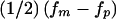Differential male and female disease penetrances.—The likelihood can be extended to model differential male and female disease penetrances. The likelihood is parameterized with respect to the combinations of disease penetrance, given the sex of the individual and the parental origin of the disease gene(s) (i.e., f_g,m= disease penetrance, given that the individual is a girl and that the disease is maternally transmitted; f_b,m= disease penetrance, given that the individual is a boy and that the disease is maternally transmitted; and f_g,p and f_b,p, similarly defined). Given this parameterization, the null hypotheses are either H₀:f_g,m=f_b,m or H₀:f_g,p=f_b,p, for testing for sex-based disease liability and either maternal or paternal effect, respectively.

This approach would be useful for study of sex-based threshold models that are well known in classical genetics. Threshold models in general have an underlying liability distribution for the disease; that is, when the liability threshold is crossed, the disease is expressed. For a sex-based model, the liability threshold differs, depending on the sex of the individual. One such disease is pyloric stenosis, a disorder that is manifested shortly after birth and that is characterized by a narrowing or obstruction of the pylorus. The prevalence of the disease is much higher in males than in females, affecting 1/200 males and 1/1,000 females in a sample of individuals of European descent (Jorde et al. 2000). This implies that females have a higher liability threshold and that, to exhibit the disease, must therefore be exposed to more “disease-causing” factors. Another disease for which this approach could be useful is panic disorder, in which there is an established sex-based disease liability and a potential parental effect. Panic disorder is a psychiatric disease characterized by spontaneous and repeated panic attacks often accompanied by agoraphobia. The risk of developing panic disorder in females has been estimated to be twice that in males, and this 2:1 (female:male) sex ratio has been observed cross-culturally (Bland et al. 1988; Robins et al. 1988; Keyl and Eaton 1990; Eaton et al. 1994). Also, there is suggestive evidence for a maternal effect in panic disorder, in which a nominally significant difference (greater than the expected 2:1) in the sex ratio has been observed, when the disease is transmitted maternally (Haghighi et al. 1999). The parent-of-origin analysis conducted by Haghighi et al. (1999), was based on a simple counting approach. Application of the full likelihood model developed here to the same collection of families with panic disorder would make it possible to test for both sex-based disease penetrance and parent-of-origin effect.

Multigenerational pedigrees.—The existing likelihood models for parent-of-origin effects are limited to nuclear families or small- to moderate-size multigenerational pedigrees (Strauch et al. 2000). However, since we have derived the exact likelihoods for all possible parental MTs (table 1), these likelihood calculations can be extended straightforwardly to general pedigree structures, by application of the clipping algorithm (Elston and Stewart 1971; Ott 1974). Here, all the information concerning the pattern of disease transmission across successive generations is captured for testing for parent-of-origin effect. This approach would be more robust than the existing methods, since it would handle pedigrees of arbitrary size and structure. The likelihood model with ascertainment cannot in general be extended to general pedigree structures, because of the inherent intractability of incorporating the general ascertainment model in the likelihood for extended pedigrees (Vieland and Hodge 1995), except in the special case of single ascertainment (Hodge and Vieland 1996).

More-complex models.—Although we have adopted a single-locus dominant genetic model with reduced penetrance, the likelihood model can be extended to allow for more-complex models that approximate the genetic etiology of complex diseases. For example, these models may allow for phenocopies, genetic heterogeneity (i.e., locus or allelic heterogeneity), epistasis (i.e., interaction among multiple genes), and/or a variety of environmental factors.

Of particular interest will be the attempt to extend the likelihood formulation to two (or more) loci, with recombination fraction, so as to be able to perform linkage studies. Investigators have attempted to model parent-of-origin effect in linkage analysis by maximizing the LOD score over separate male and female recombination fractions. The difference in the estimates of the male and female recombination fractions was used as an indicator of potential parental effect. For modeling of genomic imprinting, the male and female recombination fractions were maximized separately, when depending on the sex of the assumed imprinted parent, the corresponding recombination fraction was fixed at 1/2 (Smalley 1993; Strauch et al. 2000). This means that, in the likelihood calculation, the nonpenetrant children of an imprinting parent are considered to be recombinants. However, this approach does not account for the situation in which, in successive generations, these nonpenetrant children can be disease carriers and may have affected children (Strauch et al. 2000). Another approach at modeling of parental effect could involve assigning of liability classes for maternal- and paternal-transmission penetrances separately, depending on the observed parental mating phenotypes. However, the liability classes cannot be accurately assigned when the MT is ambiguous with respect to maternal or paternal transmission (i.e., both parents either are affected or are unaffected). An advantage of the likelihood formulation derived here is that it allows for all those combinations and possibilities accurately, weighting their probabilities appropriately.

Strauch et al. (2000) have modeled parent-of-origin effect (specifically genomic imprinting) in parametric linkage analysis, by replacing the single-heterozygous penetrance parameter with two penetrance parameters corresponding to maternal- and paternal-transmission penetrances. Although this approach has been parameterized in the context of genomic imprinting, it is in principle equivalent to our likelihood formulation of the parent-of-origin–effect model without ascertainment (model I). This method has been incorporated as an extension to the GENEHUNTER program (Kruglyak et al. 1995, 1996), referred to as “GENEHUNTER-IMPRINTING.” Also note that that program was tested on a single real data set in which the underlying genetic model was unknown. One of the strengths of our study is that we tested our program with extensive simulations, in which the underlying genetic model is known.

Appendix A: Demonstration That, When δ Is the Only Parameter of Interest, δ Estimated under Single Ascertainment Is Identical to δ Estimated under Random Ascertainment

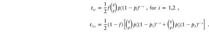
We consider nuclear families with s children, and to begin we consider the special case of a rare dominant disease, so that there are only three phenotypic MTs: affected mother × unaffected father (MT=1); unaffected mother × affected father (MT=2); and both parents unaffected (MT=3). Let r denote the number of affected children, r=1,…,s. As in the text, f denotes the mean penetrance (and, thus, the penetrance that applies to the parents, since the sexes of their respective transmitting parents are not known). Let f₁ and f₂ denote maternal- and paternal-transmission penetrances, respectively, and δ≡(1/2)(f₁-f₂), as in the text. For convenience, we also define p_i≡(1/2)f_i as the segregation ratio for the mother or father, respectively.

Probabilities under Single Ascertainment

We define u_i,r as the probability that a family of MT=i, with r affected children, is in the data set—that is,

Under single ascertainment, these probabilities are as follows:

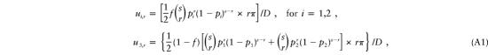where π represents the probability (π→0 under single ascertainment) that an affected child becomes a proband, and where D, the denominator, represents the sum of the numerators of all the u_i,r, summed over i=1,2,3 and over r=1,…,s. (The “1/2” is an indication that, a priori, the transmitting parent is equally likely to be the mother or the father in this model.) Algebraic manipulation reveals that D=(1/2)πs(p₁+p₂). On the basis of the above definitions, p₁=(1/2)(f+δ) and p₂=(1/2)(f-δ), so the denominator becomes D=(1/2)πsf. Thus, in the probabilities u_i,r, the parameter of interest, δ, appears only in the p_i terms in the numerators. We now rewrite the probabilities in equation (A1), to explicitly show the role played by δ:

where A₁, A₂, and A₃ represent “constant” terms that do not contain δ.

Probabilities under “Wrong” Ascertainment Model

Let t_i,r represent the “wrong” probability that a family of MT=i, with r affected children, is in the data set—that is,

We derive these probabilities:

Again, we rewrite these probabilities as functions of δ:

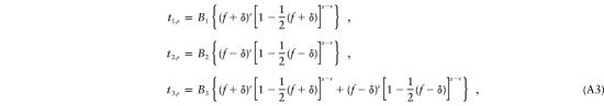where B₁, B₂, and B₃ represent constant terms that do not contain δ.

Equivalence of the Two Likelihoods

Let n_i,r represent the number of families in the data set of MT=i, with r affected children. The log-likelihood for the data set under single ascertainment is given by

whereas under the wrong ascertainment model it is

There are two differences between equations (A4) and (A5), but neither difference affects . The first difference is that equation (A4) uses u_i,r, whereas equation (A5) uses t_i,r. However, equations (A2) and (A3) reveal that, although the probabilities u_i,r and t_i,r are not respectively equal, they are proportional in δ. Hence, equations (A4) and (A5) will both maximize at the same value of δ. The other difference is that the sum in equation (A5) includes the case r=0, whereas the sum in equation (A4) does not. However, n_i,0=0 for all i, so that difference is immaterial.

More General Result

Above, we have derived the explicit probabilities for nuclear families with only three possible MTs, so as to show the algebra. However, the more general reasoning is that, under single ascertainment, the “denominator” in equation (A1) is always proportional to the prevalence of a proband (Hodge and Vieland 1996), and this prevalence is not a function of δ. Hence, as long as we are maximizing only with respect to δ, the “wrong” likelihood based on random ascertainment will yield the same as the correct likelihood based on single ascertainment.

References

- Battaglia M, Bertella S, Bajo S, Binaghi F, Ogliari A, Bellodi L (1999) Assessment of parent-of-origin effect in families unlineally affected with panic disorder-agoraphobia. J Psychiatr Res 33:37–39 [DOI] [PubMed] [Google Scholar]
- Bland RC, Orn H, Newman SC (1988) Lifetime prevalence of psychiatric disorders in Edmonton. Acta Psychiatr Scand Suppl 338:24–32 [DOI] [PubMed] [Google Scholar]
- Constancia M, Pickard B, Kelsey G, Reik W (1998) Imprinting mechanisms. Genome Res 8:881–900 [DOI] [PubMed] [Google Scholar]
- Eapen V, O’Neill J, Gurling HM, Robertson MM (1997) Sex of parent transmission effect in Tourette’s syndrome: evidence for earlier age at onset in maternally transmitted cases suggests a genomic imprinting effect. Neurology 48:934–937 [DOI] [PubMed] [Google Scholar]
- Eaton WW, Kessler RC, Wittchen HU, Magee WJ (1994) Panic and panic disorder in the United States. Am J Psychiatry 151:413–420 [DOI] [PubMed] [Google Scholar]
- Elston RC, Stewart J (1971) A general model for the genetic analysis of pedigree data. Hum Hered 21:523–542 [DOI] [PubMed] [Google Scholar]
- Ewens WJ, Shute NC (1986) The limits of ascertainment. Ann Hum Genet 50:399–402 [DOI] [PubMed] [Google Scholar]
- Falls JG, Pulford DJ, Wylie AA, Jirtle RL (1999) Genomic imprinting: implications for human disease. Am J Pathol 154:635–647 [DOI] [PMC free article] [PubMed] [Google Scholar]
- Gershon ES, Badner JA, Detera-Wadleigh SD, Ferraro TN, Berrettini WH (1996) Maternal inheritance and chromosome 18 allele sharing in unilineal bipolar illness pedigrees. Am J Med Genet 67:202–207 [DOI] [PubMed] [Google Scholar]
- Greenberg DA (1986) The effect of proband designation on segregation analysis. Am J Hum Genet 39:329–339 [PMC free article] [PubMed] [Google Scholar]
- Haghighi F, Fyer AJ, Weissman MM, Knowles JA, Hodge SE (1999) Parent-of-origin effect in panic disorder. Am J Med Genet 88:131–135 [PubMed] [Google Scholar]
- Haghighi F, Hodge SE (1999) Searching for parent-of-origin effect in complex disorders. Am J Hum Genet Suppl 65:A15 [Google Scholar]
- Hodge SE, Vieland VJ (1996) The essence of single ascertainment. Genetics 144:1215–1223 [DOI] [PMC free article] [PubMed] [Google Scholar]
- Jorde LB, Carey JC, Bamshad MJ, White RL (eds) (2000) Medical Genetics. Mosby Press, St Louis [Google Scholar]
- Kato T, Winokur G, Coryell W, Keller MB, Endicott J, Rice J (1996) Parent-of-origin effect in transmission of bipolar disorder. Am J Med Genet 67:546–550 [DOI] [PubMed] [Google Scholar]
- Keyl PM, Eaton WW (1990) Risk factors for the onset of panic disorder and other panic attacks in a prospective, population-based study. Am J Epidemiol 131:301–311 [DOI] [PubMed] [Google Scholar]
- Kruglyak L, Daly MJ, Lander ES (1995) Rapid multipoint linkage analysis of recessive traits in nuclear families, including homozygosity mapping. Am J Hum Genet 56:519–527 [PMC free article] [PubMed] [Google Scholar]
- Kruglyak L, Daly MJ, Reeve-Daly MP, Lander ES (1996) Parametric and nonparametric linkage analysis: a unified multipoint approach. Am J Hum Genet 58:1347–1363 [PMC free article] [PubMed] [Google Scholar]
- Lichter DG, Jackson LA, Schachter M (1995) Clinical evidence of genomic imprinting in Tourette’s syndrome. Neurology 45:924–928 [DOI] [PubMed] [Google Scholar]
- Lightowlers RN, Chinnery PF, Turnbull DM, Howell N (1997) Mammalian mitochondrial genetics: heredity, heteroplasmy and disease. Trends Genet 13:450–455 [DOI] [PubMed] [Google Scholar]
- McMahon FJ, Stine OC, Meyers DA, Simpson SG, DePaulo JR (1995) Patterns of maternal transmission in bipolar affective disorder. Am J Hum Genet 56:1277–1286 [PMC free article] [PubMed] [Google Scholar]
- Morton NE (1959) Genetic tests under incomplete ascertainment. Am J Hum Genet 11:1–16 [PMC free article] [PubMed] [Google Scholar]
- Ott J (1974) Estimation of the recombination fraction in human pedigrees: efficient computation of the likelihood for human linkage studies. Am J Hum Genet 26:588–597 [PMC free article] [PubMed] [Google Scholar]
- Pearson CE, Sinden RR (1998) Trinucleotide repeat DNA structures: dynamic mutations from dynamic DNA. Curr Opin Struct Biol 8:321–330 [DOI] [PubMed] [Google Scholar]
- Reddy PS, Housman DE (1997) The complex pathology of trinucleotide repeats. Curr Opin Cell Biol 9:364–372 [DOI] [PubMed] [Google Scholar]
- Robins LN, Wing J, Wittchen H-U, Helzer JE, Babor TR, Burke J, Farmer A, Jablenski A, Pickens R, Regier DA, Sartorius N, Towle LH (1988) The Composite International Diagnostic Interview: an epidemiologic instrument suitable for use in conjunction with different diagnostic systems and in different cultures. Arch Gen Psychiatry 45:1069–1077 [DOI] [PubMed] [Google Scholar]
- Smalley SL (1993) Sex-specific recombination frequencies: a consequence of imprinting? Am J Hum Genet 52:210–212 [PMC free article] [PubMed] [Google Scholar]
- Stene J (1979) Choice of ascertainment model. II. Discrimination between multi-proband models by means of birth order data. Ann Hum Genet 42:493–505 [DOI] [PubMed] [Google Scholar]
- Stine OC, Xu J, Koskela R, McMahon FJ, Gschwend M, Friddle C, Clark CD, McInnis MG, Simpson SG, Breschel TS, Vishio E, Riskin K, Feilotter H, Chen E, Shen S, Folstein S, Meyers DA, Botstein D, Marr TG, DePaulo JR (1995) Evidence for linkage of bipolar disorder to chromosome 18 with a parent-of-origin effect. Am J Hum Genet 57:1384–1394 [PMC free article] [PubMed] [Google Scholar]
- Strauch K, Fimmers R, Kurz T, Deichmann KA, Wienker TF, Baur MP (2000) Parametric and nonparametric multipoint linkage analysis with imprinting and two-locus–trait models: application to mite sensitization. Am J Hum Genet 66:1945–1957 [DOI] [PMC free article] [PubMed] [Google Scholar]
- Suomalainen A (1997) Mitochondrial DNA and disease. Ann Med 29:235–246 [DOI] [PubMed] [Google Scholar]
- Tycko B, Trasler J, Bestor T (1997) Genomic imprinting: gametic mechanisms and somatic consequences. J Androl 18:480–486 [PubMed] [Google Scholar]
- Vieland VJ, Hodge SE (1995) Inherent intractability of the ascertainment problem for pedigree data: a general likelihood framework. Am J Hum Genet 56:33–43 [PMC free article] [PubMed] [Google Scholar]
- Wallace DC, Singh G, Lott MT, Hodge JA, Schurr TG, Lezza AM, Elsas LJ 2d, Nikoskelainen EK (1988) Mitochondrial DNA mutation associated with Leber’s hereditary optic neuropathy. Science 242:1427–1430 [DOI] [PubMed] [Google Scholar]
- Weinberg W (1928) Mathematische Grundlagen der Probandenmethode. Z Induktive Abstammungs-Vererbungslehre 48:179–228 [Google Scholar]