Relationship Inference from Trios of Individuals, in the Presence of Typing Error

Abstract

Misspecification of relationships and of genotype data can cause problems in linkage analyses based on genome-scan data. Previous reports have focused on pairwise relationships and a simple error model. This article considers the increased information available from the joint analysis of trios of individuals, integrating this analysis with an error model that allows for the most common genotyping errors. Given observed marker phenotypes in a genome scan, computational methods are outlined both for likelihoods of relationships and for the posterior probabilities of underlying genotypes. The methods are applied to examples from two real data sets: one has been previously well analyzed, and, hence, Mendelian inconsistencies have been removed; the other typifies the pedigree and genotype errors encountered in the initial analyses of a study. It is demonstrated that the coupling of relationship inference and error detection is quite effective, that the error model is computationally practical, and that data on a third relative can often clarify relationships.

Introduction

Misspecification of genetic data can cause serious problems by affecting the inference drawn from linkage studies. These errors may provide false evidence for linkage or obscure the true evidence for linkage. In one example, a study of dyslexia, misreporting of MZ twins as DZ twins caused false-positive evidence for linkage (Cardon et al. 1994, 1995). Errors consist of several different types. The first type is relationship misspecification. This may occur when the true relationship is unknown by the reporting parties, which could be caused by alternate paternity or adoption. Relationship misspecification can also be caused by sample mishandling on the part of the researcher, which results in sample switches or duplications. The second type of error is genotyping error. Some common sources of genotyping error include misreading of one allele as another, similarly sized allele; failure of one allele to amplify during PCR amplification, causing a heterozygote to be typed as a homozygote; and sample contamination. We include mutation as a “typing error,” since it has similar effects in data analysis. Other sources of error in genetic analysis include misspecification of allele frequencies and of marker-map distances. In this report, we focus only on genotyping error and relationship error.

Genome-screen data can be informative for identification of likely genotype errors when the phenotype violates Mendelian inheritance or causes apparent excess recombination. Ewen et al. (2000) estimate an error rate of 0.25% in a standard 10-cM genome screen and a rate of >2% in a fine-scale–mapping marker set. They estimate that individuals who, because of either preferential amplification or failure of amplification, have been falsely classified as homozygotes account for 30% of errors in a 10-cM scan and for as much as 55% of errors in the fine-scale–mapping marker set. Mistyping due to microsatellite mutation or call errors accounts for 50% of errors in the 10-cM scan and for 25% in the fine-scale–mapping marker set. Ewen et al. (2000) report that the remaining 15%–20% of errors in their lab were due to sample swaps or mishandling.

Genome-screen data can also be informative for imputation of relationships, by demonstrating both the overall amount of genetic sharing and the patterns of sharing along chromosomes. Several investigators have developed methods for using such data to identify pedigree errors in the absence of genotyping error. Göring and Ott (1997) and Boehnke and Cox (1997) independently developed methods for computing, on the basis of genetic marker data on the pair, the likelihoods of sib, half-sib, and unrelated relationships between pairs of individuals. Both of these methods assume that genotypes are known without error. Göring and Ott (1997) take a Bayesian approach to the problem by calculating posterior probabilities of alternate relationships; they also account for parental genotypes when data on one parent are present, by calculating the relationship likelihood conditional on the parental genotype. Boehnke and Cox (1997) take a likelihood-ratio approach by comparing the likelihoods. These likelihoods and posterior probabilities are calculated by assuming a hidden Markov model (HMM) for the identity-by-descent (IBD) process, for full sibs, half-sibs, MZ twins, and unrelated individuals.

Markov-chain methods have more recently been developed for the evaluation of additional types of relationships, including parent-offspring, grandparent-grandchild, first-cousin pairs, and avuncular pairs (McPeek and Sun 2000; Epstein et al. 2000). These additional relationships are useful for more-extended pedigrees, especially when not all individuals are genotyped. Epstein et al. (2000) approximate the likelihoods of the first-cousin and avuncular relationships, in which the IBD process is not Markov. For these cases, McPeek and Sun (2000) compute the exact likelihoods by constructing an augmented Markov chain and marginalizing over the IBD states of intermediate individuals.

Broman and Weber (1998) point out that likelihood calculations can be extended to allow for genotyping error. Including a genotyping-error model can improve the relationship inference when genotyping error is present. Additionally, calculating the posterior probability of the observed data for each marker can show at which markers a genotyping error is likely to have occurred. Broman (1999) applied methods that incorporate the possibility of error to the Genetic Analysis Workshop 11 data, using a simple error model, which assumes independence between the observed phenotype and true genotype, conditional on the existence of an error. Similar methods have been implemented by Douglas et al. (2000) and Epstein et al. (2000). Kumm et al. (1999) devised a more general error model, which allows the observed phenotype to depend on the true genotype, which is more appropriate than assuming that there is independence between the two.

In each of these approaches, individuals have been compared pairwise. In many genetic studies, both in sib-pair studies and in linkage studies on pedigrees, sibships of larger sizes are collected. Browning and Thompson (1999) point out that comparing three related individuals can yield information that three pairwise comparisons cannot. Addition of a third, related individual can increase the power to infer relationships correctly. Jointly examining three full sibs can identify Mendelian errors that otherwise may be missed. Some genotype errors, which do not cause Mendelian inconsistency, may also be more apparent when three siblings are considered, because the reported genotypes require additional recombinations to explain the observed data.

Here we extend the previously developed HMMs to analysis of three individuals jointly, considering relationships that are combinations of full sibs, half-sibs, MZ twins, and unrelated individuals. We allow a more general error model, to infer relationships in the presence of genotyping error and to identify those loci at which errors have occurred. We apply these methods to two sets of genome-screen data to demonstrate their usefulness. The methods developed have been implemented in ECLIPSE (Error Correcting Likelihoods in Pedigree Structure Estimation), a C++ program that computes the likelihoods (probabilities of the data) and the posterior probability of genotypes at each locus, for a variety of relationships. The source code for this program can be downloaded from the PANGAEA web site (see the Electronic-Database Information section).

Methods

Among an ordered trio of individuals, we consider relationships that are feasible combinations of the following pairwise relationships: full sibs, half-sibs, MZ twins, and unrelated individuals. This results in 25 possible relationships among the three ordered individuals, which are listed in table 1. The simplest of these relationships are three full sibs, three MZ individuals (repeated samples), and three unrelated individuals. When ordering is taken into account, there are four distinct ways to specify three half-sibs (fig. 1): the first case occurs when all three individuals share one common parent; the remaining three cases occur when one individual shares his mother with either of the other two individuals and shares his father with the remaining individual. When we cannot distinguish between maternal and paternal sharing, this results in three possible relationships of this form. The remaining 18 relationships are six combinations of the four pairwise relationships, each giving rise to three configurations of the relationship; for example, there are three ways to designate a pair of full sibs with a half-sib, because there are three possibilities with regard to which individual is the half-sib. Similar arguments hold for the remaining five relationships: a pair of full sibs with an unrelated individual, a pair of MZ twins with a full sib, a pair of MZ twins with a half-sib, a pair of MZ twins with an unrelated individual, and a pair of half-sibs with an unrelated individual.

Table 1.

Relationships Considered in the Present Study

Relationship	No. of Distinct Orderingsa
Full sibs	1
Half-sibs (one common parent)b	1
MZ twins (repeated samples)	1
Unrelated individuals	1
Half-sibs (two different parents)b	3
Two full sibs + half-sib	3
Two full sibs + unrelated individual	3
MZ twins + sib	3
MZ twins + half-sib	3
MZ twins + unrelated	3
Two half-sibs + unrelated individual	3

^aFor several of the relationships, there are three distinct ways to specify the relationship among three ordered individuals.

^bShown in figure 1.

Figure 1.

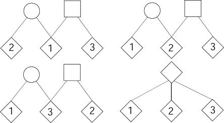
Four possible half-sib relationships. The pedigree in the lower-right quadrant shows three half-sibs with a common parent (i.e., the second relationship in table 1); each of the remaining three pedigrees shows three half-sibs with two different parents (i.e., the fifth relationship in table 1). Note that we need define only three cases when one individual shares his mother with one individual and shares his father with the other. This simplification can be made because we cannot distinguish between maternal and paternal sharing, and we assume a sex-averaged map.

For the types of relationships considered, we measure IBD relative to the previous generation; that is, for each pair of individuals we indicate whether they share their maternal and paternal alleles. The IBD states among three individuals are represented as a pair of IBD states: one describing the maternal sharing and one describing the paternal sharing. There are five patterns of maternal IBD sharing among the three individuals. These consist of the pattern in which all three individuals share their maternal allele (m₁₂₃), the pattern in which only the first and second individuals share their maternal allele (m₁₂), the pattern in which the first and third individuals share their maternal allele (m₁₃), the pattern in which the second and third individuals share their maternal allele (m₂₃), and the pattern in which none of the individuals share their maternal allele (m₀). For full sibs, only the first four maternal IBD states are possible, since there are only two choices for the allele transmitted to an offspring. We can define the five paternal IBD states (p₁₂₃, p₁₂, p₁₃, p₂₃, and p₀) analogously. Combining the maternal and paternal IBD states gives us 25 possible IBD states that describe both maternal and paternal sharing.

Now we define some notation. Let Y=(Y₁,…,Y_M) be the observed phenotypes at M markers for the three ordered individuals; thus, for each marker m, Y_m consists of the genotypes of all three individuals. We allow for genotyping error by distinguishing the marker phenotypes from the true single-locus genotypes X=(X₁,…,X_M). Finally, let I=(I₁,…,I_M) be the complete IBD states at the M markers. We will assume throughout that the allele frequencies at each marker, as well as the marker map, are known without error. If we assume that there is no genetic interference, the IBD states among individuals in the relationships described are Markov along the chromosome; that is, the IBD state at marker m, I_m, given the IBD states at all the other markers, (I₁,…,I_m-1,I_m+1,…,I_M), depends only on the states IBD at the neighboring loci, I_m-1 and I_m+1. Using this assumption we can model our data with an HMM, in which the Markov IBD process, I, cannot be observed directly but in which the observed phenotypes, Y_m, are a degradation of the underlying genotypes, X_m, whose probability is determined by I_m. The dependence among the observed and latent variables is shown in figure 2.

Figure 2.

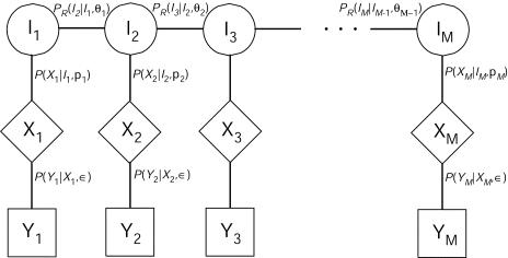
Dependence structure for HMM. The transition probabilities, P_R(I_m|I_m-1), are functions of the recombination rates, θ_m. The probability of the genotype, given the IBD state, P(X_m|I_m=j), is a function of the allele frequencies, p_m. The probability of the phenotype, given the genotype, depends on the assumed error model. Here we assume prior probability of genotyping error ε.

Using this HMM, we wish to calculate P_R(Y), the probability of the data, Y, for each particular relationship, R. These quantities will be used to compare the likelihoods of the different relationships. We will also calculate P_R(I_m|Y), the posterior probabilities of the IBD states, I_m, given the observed phenotypes. These probabilities are necessary for calculation of the posterior probability of genotyping error at each locus. To calculate these probabilities, we need, first, to calculate the transition probabilities, P_R(I_m|I_m-1), for the Markov process of IBD states along the chromosome. These transition probabilities are dependent on the relationship among the individuals and are a function of θ_m-1, the recombination frequency between marker m-1 and marker m. Furthermore, they are the product of the transition probabilities for the maternal and paternal IBD process, since these processes are independent. Table 2 describes the maternal transition probabilities for three individuals with the same mother. For the purposes of presentation, we do not distinguish between male and female maps.

Table 2.

Maternal Transition-Probability Matrix for IBD States among Three Individuals with the Same Mother

	m123	m12	m13	m23	m0
m123	θ3+(1-θ)3	θ(1-θ)	θ(1-θ)	θ(1-θ)	0
m12	θ(1-θ)	θ3+(1-θ)3	θ(1-θ)	θ(1-θ)	0
m13	θ(1-θ)	θ(1-θ)	θ3+(1-θ)3	θ(1-θ)	0
m23	θ(1-θ)	θ(1-θ)	θ(1-θ)	θ3+(1-θ)3	0
m0	0	0	0	0	1

The Baum algorithms (Baum et al. 1970) for HMMs also require the calculation of P(Y_m|I_m), the probability of the observed phenotype at locus m, given the underlying IBD state. This probability is calculated by marginalizing over all possible true genotypes, X_m:

The probability of the true genotypes, given the IBD state, P(X_m=j|I_m), is calculated under the assumption that there are Hardy-Weinberg genotypic proportions in the population (Thompson 1974). The probability of the phenotype, given the genotype, P(Y_m|X_m), is defined by the assumed error model, which is described in detail below.

To calculate P_R(Y), we use the Baum algorithm forward along the chromosome (Baum 1972). Define α_m(j|R)=P_R(Y₁,…,Y_m-1,I_m=j), the probability of the data for the first m-1 markers and the IBD state at marker m, I_m=j. Given α₁(j|R), the prior probability of IBD state j for relationship R, the proceeding values may be computed sequentially:

Finally, the probability of the data under for a particular relationship, P_R(Y), can be found: . The likelihoods of different relationships are then compared.

To calculate P_R(I_m|Y), we also proceed sequentially, this time backward along the chromosome. Let β_m(j|R)=P_R(I_m=j|Y) be the posterior probability of IBD state j at marker m, for a specified relationship; then, β_m-1(k|R) is a function of β_m(j|R), as follows:

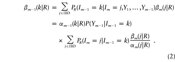These posterior IBD-state probabilities are used in calculation of the posterior probability of error for a particular relationship and error model. Note that, whereas α_m depends only on Y₁,…,Y_m-1, β_m depends on the full data Y.

When trios of individuals are considered, it is important to model genotyping errors, if there is a possibility that they exist. Failure to do so can result in incorrect inference about the underlying relationship. In particular, there are trios of genotypes that cannot occur among full siblings. Full siblings have a maximum of four distinct alleles (two maternal and two paternal) among them. Additionally, at least one pair of siblings must share their maternal allele and one pair must share their paternal allele; so, for example, the genotypes {(a,a),(a,b),(c,d)} and {(a,b),(a, c),(a,d)} cannot occur in a trio of full sibs when the alleles a, b, c, and d are unique.

Calculation of P(Y_m|I_m) can be quite computationally intensive, since it requires summation over all possible ordered three-individual genotypes, as in equation (1). At a marker with N alleles, this is a sum over {[N(N+1)]/2}³ genotypes, a value that becomes quite large for multiallelic markers; for example, a marker with 10 alleles requires a sum over >166,000 genotypes, and a marker with 15 alleles requires 1,728,000 genotypes. Since here we focus on multiallelic microsatellite markers, we constrain the error model to limit the number of terms in the sum and to make the computations feasible. For single-nucleotide polymorphisms (SNPs) or other markers with few alleles, these constraints can be relaxed. For multiallelic markers, we assume that, at any particular locus, only one error per individual may occur; that is, at least one allele per locus is typed correctly per individual. Additionally, we assume that genotyping errors in individuals occur independently over loci and over individuals, so that P(Y_m|X_m)=i=13P(Y⁽ⁱ⁾_m|X⁽ⁱ⁾_m). For each individual, we assume that the genotype is correct, with probability 1-ε, where ε is a specified genotyping-error rate. Furthermore, we let all single-allele mutations occur with equal probability. For an individual whose true genotype is homozygous (a,a), the observed phenotype is (a,b), with probability ε/(N-1), for a and b unique alleles. For a heterozygous (a,b) individual, the observed phenotype is (a,c), with probability ε/[2(N-1)], and is (b,d), with the same probability, for a and b unique, c different from b, and d different from a. Common typing errors that we particularly want to consider are the loss of one allele, usually due to either amplification failure during a PCR reaction or misreading of a single allele as another allele of similar size (Ewen et al. 2000). Although our error model is somewhat restrictive, it encompasses these common errors and allows for dependence of the observed phenotype and true genotype.

Under a given error model, we can now compute the posterior probability of latent genotypes—and, thus, of any specific typing errors at a locus in an individual or an allele. Here we focus on only the total probability, at each locus, of a typing error. In practice this is probably the most useful summary measure on which to base a decision either to ignore the data at this locus or to incur the cost of having the individuals retyped. Let P_ε(Y_m|I_m) denote the probability of the observed phenotype, given the underlying IBD state (which is calculated in eq. [1]), under the specified error model described above, with prior genotyping-error probability ε. Let β_m(j|R,ε) be the resulting posterior probability of IBD state j for relationship R, as calculated in equation (2). Then, the posterior probability that the observed phenotype is the correct genotype is

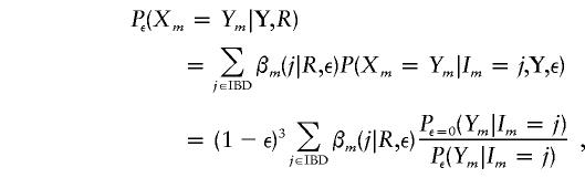since P(X_m|I_m=j,Y) = P(Y_m|X_m)P(X_m|I_m=j)/P(Y_m|I_m = j).

Results

To demonstrate the usefulness, over pairwise analysis, of analysis of trios of individuals, we here apply these methods to two different data sets. First we examine some examples from the COGA (Collaborative Study on the Genetics of Alcoholism) data set (Begleiter et al. 1995), to explore the accuracy of the inferred relationship when we have a relatively “clean” data set. The COGA data set has been well analyzed previously and is thus clean in the sense that genotypes at each locus are consistent with the reported relationships. The data consist of genotypes at 285 autosomal markers, with an average intermarker distance of ∼13 cM. For these data, we assume that observed marker genotypes are known without error; that is, we set ε, the prior probability of genotyping error, to 0. In this case, we examine putative full sibs and putative half-sibs. The second data set, lipoprotein pathophysiology grant (LPPG) (Goldstein et al. 1973), involves a pedigree from a long-standing study of cardiovascular disease for which marker genotypes for a genome scan have recently been produced. This data set may be more typical of the data initially collected in a study, since data errors have not yet been removed. The data consist of genotypes at 312 autosomal markers on 21 chromosomes, with an average intermarker distance of ∼10 cM. In this case, we examine how the modeling of genotyping error aids us in inferring the relationships among individuals.

The first example shows that, by including a third individual in the analysis, we are able to differentiate between possible relationships that are difficult to distinguish in a pairwise comparison. We first examine a pair of individuals, here denoted “A” and “B,” from the COGA data, whose reported relationship is that of half-sibs. We examine the first 100 markers, which are the markers on the first five chromosomes. Incorporating the data at these 100 markers (79 of which are typed for both A and B), we find that the data are not informative as to whether the pair of individuals are full sibs or half-sibs. The calculated log-likelihood difference between the two relationships is 0 (fig. 3A). We can increase our power to detect the true relationship by considering a third individual, C, who is a reported full sib to individual B. A pairwise analysis shows that the marker data support the reported relationship between B and C, with a log₁₀-likelihood difference, between the full-sib and half-sib hypotheses, of ∼18. Among these three individuals, there are 75 markers at which all three individuals are typed, and there are 22 markers at which one of the three genotypes is missing.

Figure 3.

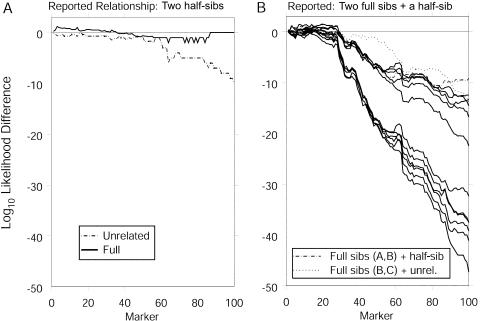
Cumulative log₁₀-likelihood differences between relationships for (A) individuals A and B, who are reported half-sibs, and (B) individuals A–C, of whom B and C are full sibs and A and B are half-sibs. For simplicity in panel B, only the curves corresponding to the 2 most likely relationships have been labeled; the unbroken curves correspond to the 11 remaining relationships that have positive likelihoods. The relationships of three full sibs and those involving MZ twins have likelihoods of 0. Each difference is relative to the reported relationship. In each case, the prior probability of genotyping error is assumed to be 0.

Considering jointly the data from the three individuals, we find that the relationship is most likely that of individual A as a half-sib to both B and C, who are full sibs. The log-likelihood difference between this relationship and the next-most-likely relationship, with A and B as full sibs and with C as a half-sib, is just over 9 (fig. 3B). Also, if we do not allow for genotyping error, we can immediately exclude 11 relationships, including that of three full sibs, because of five loci that have genotypes inconsistent with the relationship of full sibs. If we allow a prior genotyping-error probability of ε=0.02, the reported relationship (i.e., B and C as full sibs with a half-sib, A) is still most likely, with the relationship of three full sibs being the next most likely. Here, the log-likelihood difference is >5. The plots of the log-likelihood differences based on the cumulative data over increasing numbers of loci (fig. 3) show that, for the pairwise analysis of individuals A and B, the likelihood of the relationship of full sibs and the likelihood of the relationship of half-sibs remain fairly similar to each other, regardless of how many markers are considered (fig. 3A). However, when we include the third individual in the analysis, the likelihood of the reported relationship becomes well differentiated from the likelihoods of the remaining relationships, after we include the first 70 markers (fig. 3B).

Using an example involving full siblings from the COGA data, we show that inclusion of an extra sibling reduces the number of markers required for accurate inference of the relationship and increases the certainty with which we infer the relationship. The involved individuals are from the same family as in the previous example. This time, we include data from all 285 markers for individuals whom we denote “D” and “E.” Of the 285 markers, 99 are typed for both individuals. In this case, the calculated log-likelihood difference between the full-sib and half-sib hypotheses is 0.745; however, examining the cumulative log likelihoods in fig. 4A, we find that the relationship of half-sibs is more likely until we include the 208th marker. At some loci, the cumulative log-likelihood difference is >1.9 in favor of the half-sib relationship. Now we include a third individual, denoted “F,” who is reportedly a full sibling to both D and E. Considering D–F jointly, we find that there are 83 markers at which all three individuals are typed and 114 markers at which two of the three individuals are typed. The log-likelihood difference between the three-full-sibs relationship and the second-most-likely relationship, in which E is a half-sib to both F and D, is 14.88. Examining the cumulative log-likelihood differences (fig. 4B), we find that the reported relationship becomes the most likely (resulting in negative log-likelihood differences) after ∼125 markers. Thus, by including the third sibling, we improve our ability to infer the underlying relationship.

Figure 4.

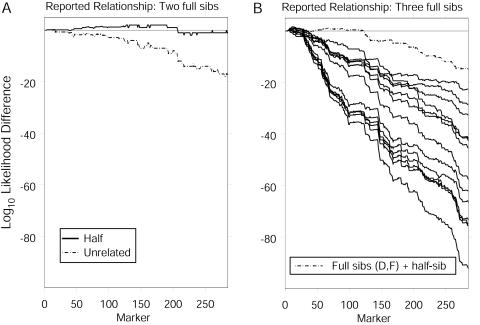
Cumulative log₁₀-likelihood differences between relationships for (A) individuals D and E, who are reported to be full sibs, and (B) individuals D–F, all three of whom are reported to be full sibs. For simplicity in panel B, only the curve corresponding the to most likely relationship is labeled; the unbroken curves correspond to the 13 remaining relationships that have positive likelihood. Each relationship with MZ twins has a likelihood of 0. Each difference is relative to the reported relationship. In each case, the prior probability of genotyping error is assumed to be 0.

We now turn our attention to an example in which the data may not be free of genotyping error. We would first like to be able to infer the correct relationship among the individuals, and, second, we would like to find probable genotyping errors. The pedigree in this example is shown in figure 5 and is part of a much larger pedigree described by Goldstein et al. (1973). To maintain the confidentiality of the subjects involved, identification and sex of the individuals may have been changed. The results are summarized in table 3. Throughout this example, we report likelihoods for ε=0.02. However, the same conclusions are drawn for ε in the range of 0.001–0.04 (data not shown). An initial pairwise comparison indicated that individual 3 was more likely a half-sib to each of its two putative siblings. A joint comparison of individuals 1–3 confirmed this result, with a log likelihood 36.3 larger than that of the second-most-likely hypothesis, that of individuals 1 and 3 as full sibs and individual 2 as a half-sib, when the prior probability of genotyping error is ε=0.02. The analysis indicated 42 markers at which the genotype was incompatible with the relationship of full sibs. When we compare individuals 1, 2, and 4 jointly, the most likely relationship is that of three full sibs, when we allow a positive probability of genotyping error. For error-free genotypes, the likelihood for the relationship of full sibs is 0. With ε=0.02, the second-most-likely relationship is that individuals 1 and 4 are full sibs and that individual 2 is their half-sib. The resulting log-likelihood difference is 62.8. The analysis indicates one marker at which the genotypes are incompatible with the full-sib relationship. Additionally, there are three other markers at which the posterior probability of error under the full-sib model is >50%. However, if we ignore the single locus with data incompatible with the relationship of full sibs and analyze the resulting data without allowing for genotyping error, the log-likelihood difference is 64.0 in favor of the relationship of full sibs. Since individuals 3 and 4 are consistent with the reported parent-offspring relationship, we conclude that there must have been a sample swap between individuals 3 and 4. Not only can we infer the correct relationships by means of this analysis, but we also have indicated with certainty one genotyping error.

Figure 5.

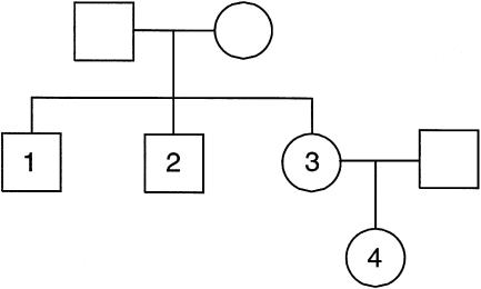
LPPG pedigree. Identifications have been changed to protect confidentiality.

Table 3.

Summary of Results for the LPPG Example, Shown in Figure 5

Individuals Considered	Individuals 1–3	Individuals 1, 2, and 4
Reported relationship	Full sibs	Two sibs (1,2) + niece (4)
Most likely relationship	Two sibs (1,2) + half-sib (3)	Three full sibs
Second-most-likely relationship	Two full sibs (1,3) + half-sib (2)	Two sibs (1,4) + half-sib (2)
Log-likelihood differencea	36.3	62.8
No. of Mendelian errorsb	42	1

^aBetween the most likely relationship and the next-most-likely relationships, when the prior probability of genotyping error is ε=0.02.

^bUnder the full-sib hypothesis.

In some instances, we can find loci at which the phenotype is incompatible with the reported (or most likely) relationship; however, in other cases, the posterior probability of error indicates loci at which the probability of error is high under the error model. Our final example explores the sensitivity, to allele frequency, of the posterior probability of error. Returning to the COGA data, we examine individuals G, H, and K, who are putative full sibs, using only the data on chromosome 1, which has 20 typed markers. Even when we allow no genotyping error, the data are considerably more probable under the full-sibs model, with a log₁₀ likelihood that is ∼2.77 larger than that of the next-most-likely relationship model. However, when we allow the model to have a prior probability of genotyping error of ε=0.02, we find that the posterior probability of error at marker 14 under the full-sibs model is quite high, 0.407. In comparison, at the remaining loci the posterior probability of error is 0.159 at marker 10 and is <0.063 at the remaining loci. Examining the genotypes at marker 14, we find that individual H is untyped, whereas individuals G and K are each homozygous for different alleles, a₁ and a₂, with allele frequencies 0.1047 and 0.0128, respectively; in other words, individual K is homozygous for a relatively rare allele, whereas individual G is homozygous for a more common allele. Thus, we may be inclined to believe that there is an error in the genotype of individual K, since, if we assume that his genotype is correct, then both his parents must carry a rare allele.

We now examine the posterior probability of error at marker 14, for the three genotypes for individual H that are consistent with the reported relationship of full sibs. These results are shown in table 4. Since we do not alter the genotypes of individuals G and K at marker 14, the parents still must be heterozygous for alleles a₁ and a₂. Despite this fact, the assumed error model causes the posterior probability of error to be quite different for the three different genotypes of individual H. For analysis of trios, the error probability appears to be sensitive to the situation when one individual is homozygous for a rare allele. The posterior probability of error is particularly high when none of the other typed individuals carries that allele (table 4). Pairwise analysis does not appear to be as sensitive to allele frequency; for example, allele frequencies have little effect on posterior probability of error when two sibs who are homozygous for the same allele are analyzed (see the probability, 0.002, in table 4.) Similarly, when individual H is heterozygous (a₁, a₂) and is compared to individual G, who is homozygous for the more common allele, or to individual K, who is homozygous for the rare allele, the posterior probability of error is similar (0.252 and 0.249, respectively). This posterior probability of error at a locus depends, of course, on the relative probability of the data, both when there is error and when there is not error, as well as on the data at linked markers. Whether the homozygous sib is so for a common or rare allele has a large effect on the absolute probability of the data but has very little effect on the relative probability either with or without error. However, there is a large effect on the specific error inferred. For individuals H and K, the likely error is in one allele of the rare homozygote, individual K. For individuals G and H, the likely error is in the rare allele in the heterozygote, individual H.

Table 4.

Posterior Probability of Error at Marker 14

	Posterior Probability of Error at Marker 14, forb
Genotype ofIndividual Ha	G and H	H and K	G and K	G, H, and K
(a1,a1)	.002	.404	.402	.451
(a1,a2)	.252	.249	.402	.324
(a2,a2)	.408	.002	.402	.091

^aFrequencies of the a₁ and a₂ alleles are 0.1047 and 0.0128, respectively.

^bIndividual G has genotype (a₁,a₁), and individual K has genotype (a₂,a₂). Results shown are based on marker data on 20 markers on chromosome 1, when the prior probability of genotyping error is ε=0.02.

The methods that we employ assume that allele frequencies, recombination rates, and genotyping-error rate are known. In practice, these quantities are estimated and are, therefore, subject to errors themselves. The previous example demonstrates that the posterior probability of error for trios is affected by the allele frequencies. However, although the likelihoods change slightly, the inferred relationship is unchanged with changes to the genotype of individual H (data not shown). Because these methods incorporate data from all markers jointly, an accurate map is important. However, for moderately spaced maps these methods are reasonably robust; for example, although the reordering of 23 widely spaced pairs of adjacent markers in the LPPG map changed the posterior probabilities of error at the reordered loci, it did not change the inferred relationships (data not shown). For only a few markers were the changes in posterior probability of error substantial, presumably because of apparent excess recombination caused by the change in marker order. The posterior probabilities of error, as well as the likelihoods, are also affected by the assumed error rate. In our analyses, we have reported results for an assumed error rate of 2%; however, we have verified that the results are qualitatively unchanged within the range of 0.1%–4%, which spans most error estimates for microsatellite markers. In practice, a sensitivity analysis may be desirable to determine the robustness of results to changes in allele frequencies, recombination frequencies, and/or error rates.

Not surprisingly, analysis of trios is more computationally complex than analysis of pairs. An analysis of a trio of individuals typed at 312 markers took 15.25 min for five different prior probabilities of genotyping error. The three pairwise analyses of the same individuals and with the same prior probabilities of genotyping error took 5.7 min. However, the majority of the computational complexity is caused by inclusion of the error model; without the genotyping-error model, 7.42 s were required for analysis of the same three individuals jointly. Note that, since the Baum algorithm is linear in the number of loci, these methods can easily be scaled to larger numbers of loci.

Discussion

Collection of genetic data may never be error free. False paternity, unrevealed adoptions, and mistakes by investigators can cause relationship misspecification in pedigrees. Genotyping methods, although increasing in accuracy, may never be perfect and will never be able to eliminate mutations. These errors can cause serious consequences in linkage studies. Therefore, data-analysis methods to minimize these errors are crucial. The coupling of typing-error detection and relationship validation can be an effective approach to both types of errors. Additionally, allowing for genotyping errors is crucial when one is validating relationships among three (or more) individuals jointly, since typing error can result in genotypes that are incompatible with the true relationship. Therefore, an adequate error model is very important. When Mendelian incompatibilities exist in the case of full sibs, this coupling of error detection and relationship validation can help us to distinguish between full sibs, among whom typing error has occurred, and more distant relationships. This has been demonstrated by the LPPG example.

A genotyping-error model must be computationally feasible and must adequately reflect the types of errors that occur in practice. Previous approaches to modeling error (Broman and Weber 1998; Broman 1999; Douglas et al. 2000; Epstein et al. 2000) have assumed independence between phenotype and genotype, conditional on the existence of an error. This model has the advantage of computational simplicity, but the assumption of independence is not accurate. Additionally, the model becomes more unrealistic when applied to trios of individuals. A more desirable approach is to allow for dependence between the phenotype and the true genotype, because, in practice, the two tend to be closely related. We introduce a framework in which a more general error may be implemented. Because we have used microsatellite markers with large numbers of alleles, we have implemented a simplified error model that allows for this dependence while maintaining computational feasibility, even when examining larger numbers of individuals jointly. By limiting the number of alleles at which an error has occurred to one per individual, we reduce the calculation of P(Y_m|I_m) to a sum on the order of N^k_m, where N_m is the number of alleles at the locus and k is the number of individuals. A more general model that allows errors at both alleles would require a sum on the order of N^2k_m, which gets quite large for multiallelic markers. Employing our simplified model, we can routinely handle markers with >20 alleles, which would be impossible for a more general model when trios of individuals are being compared. Our model adequately handles most errors for moderately spaced markers and permits feasible true genotypes for all but the most unlikely errors—for example, a trio of MZ twins (repeated samples) among whom four or more alleles are mistyped. Further investigation is needed to compare the performance and computational feasibility of this and other error models. For SNP data or microsatellites with few alleles, more-general models are computationally feasible. Investigators could weight certain types of errors more highly or even specify different error rates for each allele.

Joint analysis of trios gives more information than does analysis of pairs. This has been demonstrated, in the context of relationship validation both for half-sibs and for full sibs, by two different examples from the COGA data. Analysis of trios requires fewer markers and more clearly distinguishes relationships than does analysis of pairs. Analysis of trios is also helpful in detection of genotyping error. Mendelian errors can be detected by examination of three siblings jointly. Even when genotypes are compatible with the reported relationship, joint analysis of trios can give a very different posterior probability of error than is given by three pairwise analyses. This is demonstrated by the results in table 4. Two of the possible genotypes for individual H give a similar pattern of posterior probabilities of error in the pairwise analyses (in two of them, the posterior probability of error is ∼0.4; in the third, it is 0.002), but the two corresponding joint analyses of trios yield quite different results.

Joint analysis of trios can improve the quality of conclusions drawn with regard to genetic errors. In many studies, data on a third related individual are either available or easily collected. In the case of sib-pair studies, extra affected or unaffected sibs are often available. Current sib-pair studies are more often including information from discordant sib pairs, so extra unaffected sibs are starting to be collected whenever possible. Especially in the absence of parental data, extra siblings can often be informative, not only in detection of errors but also for the linkage study itself. These methods can also be helpful in pedigree-based linkage studies when parental data are missing; in these cases, larger sibships are routinely collected.

In principle, this approach can be extended to more-distant relationships and to joint analysis of larger numbers of individuals. McPeek and Sun (2000) and Epstein et al. (2000) have found that pairwise analysis cannot easily distinguish between half-sibs, grandparent-grandchild, and avuncular relationships. Browning and Thompson (1999) have shown that joint analysis of three individuals can distinguish between two sibs with a niece and two sibs with an aunt. Thus, extension of joint analysis to more-distant relationships may be quite useful. Although joint analysis can be extended to four or more individuals, the added computational complexity would be prohibitive for high-throughput installation.

In conclusion, the coupling of relationship validation and genotyping-error detection for trios of individuals can be quite useful. When larger sibships are available, this approach is preferable to pairwise analyses, because errors are more easily detected. The HMM of the underlying maternal and paternal IBD processes allows for easy extension to sex-specific maps. The assumed error model both is computationally feasible and models the more common genotyping errors. When other related individuals are available, joint analysis of trios may, at the very least, be applied to individuals and markers that are flagged by pairwise analysis. However, since joint analysis of trios can identify Mendelian inconsistencies, these methods may be applied to all sibships of three or more individuals. To reduce the amount of computation required, this analysis can be done first without the error model, to identify sibships with Mendelian inconsistencies or low likelihoods; then these sibships should be analyzed with the error model, to identify the loci at which errors have occurred.

References

- Baum L (1972) An inequality and associated maximization technique in statistical estimation for probabilistic functions of Markov processes. Inequalities 3:1–8 [Google Scholar]
- Baum LE, Petrie T, Soules G, Weiss N (1970) A maximization technique occurring in the statistical analysis of probabilistic functions on Markov chains. Ann Math Stat 41:164–171 [Google Scholar]
- Begleiter H, Reich T, Hesselbrock V, Porjesz B, Li TK, Schuckit M, Edenberg H, Rice J (1995) The collaborative study on the genetics of alcoholism. Alcohol Health Res World 19:228–236 [PMC free article] [PubMed] [Google Scholar]
- Boehnke M, Cox NJ (1997) Accurate inference of relationships in sib-pair linkage studies. Am J Hum Genet 61:423–429 [DOI] [PMC free article] [PubMed] [Google Scholar]
- Broman K (1999) Cleaning genotype data. Genet Epidemiol 17:S79–S83 [DOI] [PubMed] [Google Scholar]
- Broman K, Weber J (1998) Estimating pairwise relationships in the presence of genotyping errors. Am J Hum Genet 63:1563–1564 [DOI] [PMC free article] [PubMed] [Google Scholar]
- Browning S, Thompson EA (1999) Interference in the analysis of genetic marker data. Am J Hum Genet Suppl 65:A244 [Google Scholar]
- Cardon L, Smith S, Fulker D, Kimberling W, Pennington B, DeFries J (1994) Quantitative trait locus for reading disability on chromosome 6. Science 266:276–279 [DOI] [PubMed] [Google Scholar]
- ——— (1995) Quantitative trait locus for reading disability: correction. Science 268:1553 [DOI] [PubMed] [Google Scholar]
- Douglas J, Boehnke M, Lange K (2000) A multipoint method for detecting genotyping errors and mutations in sibling-pair linkage data. Am J Hum Genet 66:1287–1297 [DOI] [PMC free article] [PubMed] [Google Scholar]
- Epstein M, Duren W, Boehnke M (2000) Improved inference of relationship for pairs of individuals. Am J Hum Genet 67:1219–1231 [DOI] [PMC free article] [PubMed] [Google Scholar]
- Ewen K, Bahlo M, Treloar S, Levinson D, Mowry N, Barlow J, Foote S (2000) Identification and analysis of error types in high-throughput genotyping. Am J Hum Genet 67:727–736 [DOI] [PMC free article] [PubMed] [Google Scholar]
- Goldstein JL, Schrott H, Hazzard WR, Bierman EL, Motulsky AG (1973) Hyperlipidemia in coronary heart disease. II. Genetic analysis of lipid levels in 176 families and delineation of a new inherited disorder, combined hyperlipidemia. J Clin Invest 52:1544–1568 [DOI] [PMC free article] [PubMed] [Google Scholar]
- Göring H, Ott J (1997) Relationship estimation in affected sib pair analysis of late-onset diseases. Eur J Hum Genet 5:69–77 [PubMed] [Google Scholar]
- Kumm J, Browning S, Thompson EA (1999) Validation of pedigree data in the presence of genotyping error. Am J Hum Genet Suppl 65:A208 [Google Scholar]
- McPeek M, Sun L (2000) Statistical tests for detection of misspecified relationships by use of genome-screen data. Am J Hum Genet 66:1076–1094 [DOI] [PMC free article] [PubMed] [Google Scholar]
- Thompson EA (1974) Gene identities and multiple relationships. Biometrics 30:667–680 [PubMed] [Google Scholar]