Segmentation of Neonatal Brain MR Images using Patch-Driven Level Sets

Abstract

The segmentation of neonatal brain MR image into white matter (WM), gray matter (GM), and cerebrospinal fluid (CSF), is challenging due to the low spatial resolution, severe partial volume effect, high image noise, and dynamic myelination and maturation processes. Atlas-based methods have been widely used for guiding neonatal brain segmentation. Existing brain atlases were generally constructed by equally averaging all the aligned template images from a population. However, such population-based atlases might not be representative of a testing subject in the regions with high inter-subject variability and thus often lead to a low capability in guiding segmentation in those regions. Recently, patch-based sparse representation techniques have been proposed to effectively select the most relevant elements from a large group of candidates, which can be used to generate a subject-specific representation with rich local anatomical details for guiding the segmentation. Accordingly, in this paper, we propose a novel patch-driven level set method for the segmentation of neonatal brain MR images by taking advantage of sparse representation techniques. Specifically, we first build a subject-specific atlas from a library of aligned, manually segmented images by using sparse representation in a patch-based fashion. Then, the spatial consistency in the probability maps from the subject-specific atlas is further enforced by considering the similarities of a patch with its neighboring patches. Finally, the probability maps are integrated into a coupled level set framework for more accurate segmentation. The proposed method has been extensively evaluated on 20 training subjects using leave-one-out cross validation, and also on 132 additional testing subjects. Our method achieved a high accuracy of 0.919±0.008 for white matter and 0.901±0.005 for gray matter, respectively, measured by Dice ratio for the overlap between the automated and manual segmentations in the cortical region.

1. Introduction

Accurate segmentation of neonatal brain MR images is essential in the study of infant brain development. A large amount of work has been dedicated to the segmentation of adult brain MRI, resulting in many successful methods and also freely-available software packages (Ashburner and Friston, 2005; Cocosco et al., 2003a, b; Fischl et al., 2002; Geffroy et al., 2002; Han et al., 2004; Shattuck and Leahy, 2002; Zhang et al., 2001). However, to date, there is limited publicly available software for neonatal brain MR image segmentation. In fact, segmentation of newborn brain MRI is considerably more difficult than that of adult brain MRI (Gui et al., 2012; Prastawa et al., 2005; Weisenfeld and Warfield, 2009; Xue et al., 2007), due to the lower tissue contrast, severe partial volume effect (Xue et al., 2007), high image noise (Mewes et al., 2006), and to dynamic white matter myelination (Weisenfeld and Warfield, 2009).

In the past several years, more efforts were put into neonatal brain MRI segmentation (Anbeek et al., 2008; Gui et al., 2012; Leroy et al., 2011; Merisaari et al., 2009; Wang et al., 2011; Warfield et al., 2000; Xue et al., 2007), prompted by the increasing availability of neonatal images. Most proposed methods are atlas-based (Cocosco et al., 2003b; Prastawa et al., 2005; Shi et al., 2009; Shi et al., 2011a; Shi et al., 2010; Song et al., 2007; Warfield et al., 2000; Weisenfeld et al., 2006; Weisenfeld and Warfield, 2009). An atlas can be generated from manual or automated segmentation of an individual image, or a group of images from different individuals (Kuklisova-Murgasova et al., 2011; Shi et al., 2011b). For example, Prastawa et al. (Prastawa et al., 2005) generated an atlas by averaging three semi-automatically segmented neonatal brain images and then integrated it into the expectation-maximization (EM) scheme for tissue classification. Bhatia et al. (Bhatia et al., 2004) averaged all images as an atlas after group-wise registration of all images in a population. Warfield et al. (Warfield et al., 2000) proposed an age-specific atlas that was generated from multiple subjects using an iterative tissue-segmentation and atlas-alignment strategy to improve neonatal tissue segmentation. In our previous work, we constructed population-based infant atlases (Shi et al., 2011b) and integrated them into a level set framework for neonatal brain segmentation (Wang et al., 2011). However, one common limitation of all these atlas construction methods is that the complex brain structures, especially those in the cortical regions, are generally diminished after atlas construction due to the simply averaging of a population of images, which often have considerable inter-subject anatomical variability even after non-linear registration.

As proposed in (Aljabar et al., 2009; Shi et al., 2009), a subject-specific atlas, which can be constructed from images that are similar to the to-be-segmented image or from a large population of images (Ericsson et al., 2008), produces more accurate segmentation results than the population-based atlases. Thus, Shi et al. (Shi et al., 2009) proposed a novel approach for neonatal brain segmentation by utilizing an atlas built from the longitudinal follow-up image of the same subject (i.e., the image scanned at one or two years of age) to guide neonatal image segmentation. In (Wang et al., 2013), a novel longitudinally guided level set method was proposed for consistent neonatal image segmentation by utilizing the segmentation results of the follow-up image. In practice, however, many neonatal subjects do not have longitudinal follow-up scans.

Besides, most of the above-mentioned methods perform segmentation on a voxel-by-voxel basis. Recently, patch-based methods (Coupé et al., 2012a; Coupé et al., 2012b; Coupé et al., 2011; Eskildsen et al., 2012; Rousseau et al., 2011) have been proposed for label fusion and segmentation. Their main idea is to allow multiple candidates (usually in the neighborhood) from each template image and to aggregate them based on non-local means (Buades et al., 2005). Different from multi-atlas based label fusion algorithms (Asman and Landman, 2012; Langerak et al., 2010; Sabuncu et al., 2010; Wang et al., 2012; Warfield et al., 2004), which require accurate non-rigid image registration, these patch-based methods are less dependent on the accuracy of registration, thus even the low-accuracy rigid registration can also be applied. This technique has been successfully validated on brain labeling (Rousseau et al., 2011) and hippocampus segmentation (Coupé et al., 2011) with promising results.

Recently, patch-based sparse representation has attracted rapidly growing interest. This approach assumes that image patches can be represented by sparse linear combination of image patches in an over-complete dictionary (Elad and Aharon, 2006; Gao et al., 2012; Mairal et al., 2008b; Winn et al., 2005; Yang et al., 2010). This strategy has been applied to a good deal of image processing problems, such as image denoising (Elad and Aharon, 2006; Mairal et al., 2008b), image in-painting (Fadili et al., 2009), image recognition (Mairal et al., 2008a; Winn et al., 2005), and image super-resolution (Yang et al., 2010), achieving the state-of-the-art performance. In this paper, we propose a novel strategy via patch-based sparse representation for neonatal brain image segmentation. Specifically, we first construct a subject-specific atlas, which is based on a set of aligned and manually segmented neonatal images. Each patch in the subject can then be sparsely represented by patches in the dictionary, and thus this patch will have a similar tissue label with the selected patches according to their respective sparse coefficients. To ensure that the probability is spatially consistent, we further refine the tissue probability maps by considering the similarities between the current patch and its neighboring patches. Finally, the obtained tissue probability maps are integrated into a level set framework for more accurate segmentation of neonatal brain MRI. Note that, although the detection of myelination and maturation of white matter is also very important in the early brain development study (Gui et al., 2012; Prastawa et al., 2005; Weisenfeld and Warfield, 2009), this paper focuses on segmentation of neonatal brain images into general GM, WM, and CSF, where WM contains both myelinated and unmyelinated WM, and GM contains both cortical and subcortical GM.

The remainder of this paper is organized as follows. In Section 2, we review our previous method and its limitations. The proposed method is introduced in Section 3. The experimental results are presented in Section 4, followed by discussions in Section 5.

2. Background: Coupled Level Set (CLS)

In this section, we will first review our previous method (Wang et al., 2011) and then point out its major limitations. Let Ω be the image domain and C be a closed subset in Ω, which divides the image domain into disjoint partitions Ω_j, j ∈ {WM, GM, CSF, BG} such that Ω = U_j Ω_j . Our previous coupled level set (CLS) method combines the local intensity information (Wang et al., 2009), atlas spatial prior P_j, and cortical thickness constraint into a level set based framework. For each voxel x in image I, let 𝒩(x) be the neighborhood of voxel x. For y ∈ 𝒩 (x), its intensity distribution model on the j-th tissue can be parameterized by a normal distribution Θ_j(y) with the local mean u_j(y) and the variance ${\sigma }_j^{2\left(y\right)}$ (Wang et al., 2009). Then, the probability of intensity I(x) belonging to the j-th tissue type, denoted by p_j,y (I(x)), can be estimated as

$$p_{j,y}\left(I\left(x\right)\right)=\frac{1}{\sqrt{2\pi }{\sigma }_j\left(y\right)}exp\left(-\frac{{(u_j\left(y\right)-I\left(x\right))}^2}{2{\sigma }_j^2\left(y\right)}\right)$$ (1)

Therefore, using all y ∈ 𝒩 (x), the probability of intensity I(x) belonging to the j-th tissue type, $p_j^{LGD}\left(x\right)$, can be jointly estimated by averaging the local Gaussian distributions (LGD)

$$p_j^{LGD}\left(x\right)=\frac{1}{|\mathcal{N}\left(x\right)|}\underset{y\in \mathcal{N}\left(x\right)}{\Sigma }{p}_{j,y}\left(I\left(x\right)\right)$$ (2)

where |𝒩 (x)| is the total number of voxels in the neighborhood. Then, by considering also the population-atlas prior P_j, the overall probability of the voxel x belonging to the j-th tissue type, $P_j^{LGD\_Prior}\left(x\right)$, can be estimated by,

$$P_j^{LGD\_Prior}\left(x\right)=\frac{1}{Z_1\left(x\right)}\underset{y\in \mathcal{N}\left(x\right)}{\Sigma }\underset{population-basedatlas}{\underbrace{P_j\left(x\right)}}\underset{LGD}{\underbrace{p_{j,y}\left(I\left(x\right)\right)}}$$ (3)

where Z₁ (x) = ∑_j ∑_y∈𝒩(x) is a normalization constant to ensure ${\Sigma }_j{P}_j^{LGD\_Prior}\left(x\right)=1$. Therefore, the data-driven energy term E^led_prior that we minimize can be defined as follows,

$$E^{LGD\_Prior}\left(C\right)=-\underset{j}{\Sigma }\underset{x\in {\Omega }_j}{\Sigma }log{P}_j^{LGD\_Prior}\left(x\right)$$ (4)

This data-driven term, combined with the cortical thickness constraint term (Wang et al., 2011; Wang et al., 2013), was integrated into a coupled level set framework for neonatal image segmentation in our previous CLS method (Wang et al., 2011). Note that the data-driven energy term E^lgd_prior in Eq. (4) looks different from the energy term in our previous work (Wang et al., 2011; Wang et al., 2013). However, as shown in Appendix 1, the minimization problem of E^lgd_prior can be converted to the minimization problem of the energy functional in our previous work (Wang et al., 2011; Wang et al., 2013).

However, there are two major limitations in our previous CLS method. First, the prior P was derived by warping a population-based infant atlas. One limitation is that the population-based atlas may not be representative of a single subject in the regions with high inter-subject variability and thus leads to a low capability for guiding the tissue segmentation. For example, it can be seen that the population-based atlas (shown in the 2nd row of Fig. 1) is far from accurate, especially at the cortical regions. Second, in Eq. (3), only the voxel-wise intensity information was used to estimate the probability. However, in the T2 neonatal MR images, due to the partial volume effect, the intensities of voxels on the boundary between CSF and GM are similar to those of the WM, which may lead to incorrect tissue labeling. For illustration, the 3rd row of Fig. 1 shows the probability maps (of WM, GM, and CSF) obtained by using $P_j^{LGD\_Prior}$ (Eq. (3)). It can be observed that these probability maps are spatially inconsistent and noisy (see red arrows in Fig. 1).

Figure 1.

Illustration of the tissue probability maps estimated by different methods. The first row is the original T2 image. The 2nd and 3rd rows demonstrate the two limitations of the coupled level set (CLS) method (Wang et al., 2011): population-based atlas is far from accurate and the CLS uses only the voxel-wise intensity information to estimate the probability which results in spatial inconsistency. The last two rows show the proposed subject-specific atlases, without and with the enforced spatial consistency. The right color bar indicates the probability ranging from 0 to 1.

To deal with these limitations, in the following paragraphs, we propose a novel patch-based method for neonatal image segmentation. Instead of considering only the voxel-wise information in the coupled level set (CLS) method, we now consider the patch-level information, based on the sparse representation technique for building the tissue probability maps. It is worth noting that in this paper we propose a subject-specific atlas to overcome the first limitation of using the population-based atlas in CLS, and then utilize the patch-level information, based on the sparse representation, to overcome the second limitation of using only the voxel-wise intensity information for estimating tissue probability maps in CLS.

3. Materials and method

The proposed method consists of three main steps as summarized in Fig. 2. Its details are presented in the following sections, i.e., construction of the subject-specific atlas from the template images (Section 3.2), enforcing the spatial consistency for the probability maps (Section 3.3), and further integrating it into a coupled level set framework (Section 3.4) for tissue segmentation.

Figure 2.

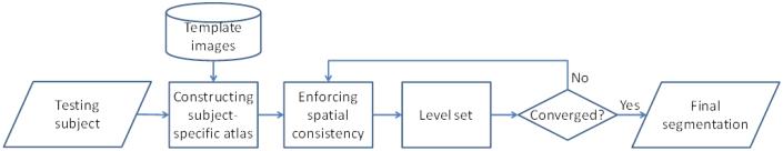
The flowchart of the proposed method. It consists of three main steps: 1) constructing the subject-specific atlas from the template images; 2) enforcing the spatial consistency for the probability maps and 3) further integrating it into a coupled level set framework for tissue segmentation.

3.1 Data Description and library construction

The library is constructed from N (N = 20) normal neonatal subjects used as template images. Images were acquired on a Siemens head-only 3T scanner (Allegra, Siemens Medical System, Erlangen, Germany) with a circular polarized head coil. T2 images of 70 transverse slices were acquired with turbo spin-echo (TSE) sequences: TR = 7380 ms, TE = 119 ms, Flip Angle = 150, and resolution = 1.25×1.25×1.95 mm³. The gestational age of the neonates was 38.6±2.6 weeks at birth and 41.5±1.7 weeks at MR scanning. T2 images were resampled to 1× 1 × 1mm³. Standard preprocessing steps were performed before segmentation, including skull stripping (Shi et al., 2012), intensity inhomogeneity correction (Sled et al., 1998), and removal of the cerebellum and brain stem by using in-house tools, where a template was employed to mask out the cerebellum and brain stem after a nonlinear registration. Ideally, one would use MR images with manually segmentation results to create the library, which, however, is heavily time consuming. We took a more practical approach to first generate reasonable segmentation results by the publicly available iBEAT software (http://www.nitrc.org/projects/ibeat/), and then perform manual edition to correct errors. Three representative intensity images with their corresponding manual segmentation results, randomly selected from those 20 subjects, are shown in Fig. 3.

Figure 3.

Three randomly-selected subjects and their corresponding manual segmentation results.

3.2 Constructing a subject-specific atlas from the aligned template images

To construct a subject-specific atlas for a testing image I, N template images Iⁱ and their corresponding segmentation maps Lⁱ (i = 1, ..., N) are first linearly aligned onto the space of the testing image. Then, for each voxel x in the testing image I, its intensity patch (taken from w × w × w neighborhood) can be represented as a w × w × w dimensional column vector m_x. Furthermore, its patch dictionary can be adaptively built from all N aligned templates as follows. First, let 𝒩ⁱ(x) be the neighborhood of voxel x in the i-th template image Iⁱ, with the neighborhood size as w_p × w_p × w_p . Then, for each voxel y ∈ 𝒩ⁱ(x) we can obtain its corresponding patch from the i-th template, i.e., a w × w × w dimensional column vector ${\mathit{m}}_y^i$. By gathering all these patches from w_p × w_p × w_p neighborhoods of all N aligned templates, we can build a dictionary matrix D_x, where each patch is represented by a column vector and normalized to have the unit ℓ2 norm (Cheng et al., 2009; Wright et al., 2010). To represent the patch m_x of voxel x in the testing image by the dictionary D_x, its sparse coefficient vector α can be estimated by minimizing the non-negative Elastic-Net problem (Zou and Hastie, 2005),

$$\underset{\alpha \ge 0}{\underset{\alpha }{min}}\frac{1}{2}\left|\right|{\mathit{m}}_x-{\mathit{D}}_x\alpha |{|}_2^2+{\lambda }_1|\left|\alpha \right|{|}_1+\frac{{\lambda }_2}{2}\left|\right|\alpha |{|}_2^2$$ (5)

The first term is the data fitting term, the second term is the ℓ1 regularization term which is used to enforce the sparsity constraint on the reconstruction coefficients α, and the last term is the ℓ2 smoothness term to enforce the similarity of coefficients for similar patches. Eq. (5) is a convex combination of ℓ1 lasso (Tibshirani, 1996) and ℓ2 ridge penalty, which encourages a grouping effect while keeping a similar sparsity of representation (Zou and Hastie, 2005). In our implementation, we use the LARS algorithm (Efron et al., 2004), which was implemented in the SPAMS toolbox (http://spams-devel.gforge.inria.fr), to solve the Elastic-Net problem. Each element of the sparse coefficients α, i.e., ${\alpha }_y^i$, reflects the similarity between the target patch m_x and the patch ${\mathit{m}}_y^i$ in the patch dictionary (Cheng et al., 2009). Based on the assumption that similar patches should share similar tissue labels, we use the sparse coefficients α to estimate the probability of the voxel x belonging to the j-th tissue, i.e.,

$$P_j\left(x\right)=\frac{1}{Z_2\left(x\right)}\underset{i}{\Sigma }\underset{y\in {\mathcal{N}}^i\left(x\right)}{\Sigma }{\alpha }_y^i{\delta }_j\left(L^i\left(y\right)\right)$$ (6)

where $Z_2\left(x\right)={\Sigma }_i{\Sigma }_j{\Sigma }_{y\in {\mathcal{N}}^i\left(x\right)}{\alpha }_y^i{\delta }_j\left(L^i\left(y\right)\right)$ is a normalization constant to ensure Σ_j P_j(x) = 1 and δ_j(Lⁱ(y)) is defined as

$${\delta }_j\left(L^i\left(y\right)\right)=\{\begin{array}{c}1,L^i\left(y\right)=j;\hfill \\ 0,L^i\left(y\right)\ne j.\hfill \end{array}\phantom{\}}$$

By visiting each voxel in the testing image I, we can build a patient-specific atlas. The 4th row of Fig. 1 shows an example of the proposed subject-specific atlas. Compared with the population-based atlas used in the coupled level set (CLS) (as shown in the 2nd row), the proposed subject-specific atlas contains much richer anatomical details, especially at the cortical regions.

3.3 Enforcing spatial consistency in the testing image space

In the previous section, the tissue probability of each voxel is estimated independently for the neighboring points, which may result in spatial inconsistency. To address this issue, we propose the following strategy to refine the tissue probability to be spatially consistent. As shown in Fig. 4, for each voxel x in the testing image (red point), we constrain its tissue probability to be spatially consistent with all the voxels y (blue points) in its neighborhood N(x) (yellow circle). Following the notation in the previous section, for each voxel x in the testing image I, its intensity patch can be represented as a w × w × w dimensional column vector m_x. For each neighboring voxel y ∈ 𝒩 (x), we can also obtain its corresponding patch with same dimension, i.e., a column vector m_y. By gathering all these patches from the w_p × w_p × w_p neighborhood, we can build a dictionary matrix ${\mathit{D}}_x^{\prime }$, where each patch is represented by a column vector and normalized to have the unit ℓ2 norm (Cheng et al., 2009; Wright et al., 2010). It should be noted that all patches here are from the testing image itself, while the patches in Section 3.2 are derived from the aligned template images. Similar to Eq. (5), to represent the patch m_x of voxel x in the testing image by the dictionary ${\mathit{D}}_x^{\prime }$, its sparse coefficient vector α^′ could be estimated by minimizing the non-negative Elastic-Net problem (Zou and Hastie, 2005),

$$\underset{\alpha \prime \ge 0}{\underset{\alpha \prime }{min}}\frac{1}{2}\left|\right|{\mathit{m}}_x-{\mathit{D}}_x^{\prime }\alpha \prime |{|}_2^2+{\lambda }_1||\alpha \prime |{|}_1+\frac{{\lambda }_2}{2}\left|\right|\alpha \prime |{|}_2^2$$ (7)

Each element of sparse coefficients α′, i.e., ${\alpha }_y^{\prime }$ reflects the similarity between the testing patch m_x and the neighboring patch m_y in the dictionary. Before proposing the new strategy to estimate the probability, we recall the probability estimated by CLS:

$$P_j^{LGD\_prior}\left(x\right)=\frac{1}{Z_1\left(x\right)}\underset{y\in \mathcal{N}\left(x\right)}{\Sigma }\underset{population-basdatlas}{\underbrace{P_j\left(x\right)}}\underset{LGD}{\underbrace{p_{j,y}\left(I\left(x\right)\right)}}$$ (8)

It can be deduced that CLS only considers the voxel-wise intensity information and all the neighboring voxels contributed equally to the probability, which could result in spatial inconsistency as shown in Fig. 1. Here, we propose the following scheme to enforce the spatial consistency, which takes advantage of the sparse coefficient ${\alpha }_y^{\prime }$ based on the patch similarity,

$$P_j^{Patch\_LGD\_Prior}\left(x\right)=\frac{1}{Z_3\left(x\right)}\frac{1}{\underset{y\in \mathcal{N}\left(x\right)}{\Sigma }{\alpha }_y^{\prime }}\underset{y\in \mathcal{N}\left(x\right)}{\Sigma }\underset{patchsimilarity}{\underbrace{{\alpha }_y^{\prime }}}\underset{subject-specificatlas}{\underbrace{P_j\left(x\right)}}\underset{LGD}{\underbrace{p_{j,y}\left(I\left(x\right)\right)}}$$ (9)

where $Z_3\left(x\right)={\Sigma }_j\frac{1}{{\Sigma }_{y\in \mathcal{N}\left(x\right)}{\alpha }_y^{\prime }}{P}_j\left(x\right)p_{j,y}\left(I\left(x\right)\right)$ is a normalization constant to ensure ${\Sigma }_j{P}_j^{Patch\_LGD\_Prior}\left(x\right)=1$. Compared with the CLS method (Eq. (3)), there are two advantages of the proposed method, 1) a subject-specific atlas (P_j) is utilized, instead of the population-based atlas; 2) patch information (${\alpha }_y^{\prime }$) is also incorporated instead of only the voxel-wise information. Therefore, the energy that we will minimize is given by,

$$E^{Patch\_LGD\_Prior}\left(C\right)=\underset{j}{\Sigma }\underset{x\in {\Omega }_j}{\Sigma }-\log P_j^{Patch\_LGD\_Prior}\left(x\right).$$ (10)

Figure 4.

Enforcing spatial consistency in the probability maps. Each voxel y ∈ 𝒩 (x) will adaptively contribute to the probability of voxel x based on their patches similarities.

3.4 Level set segmentation

In level set methods, the set of contours C can be represented by the union of the zero level sets and the image partitions Ω_j can be formulated by the level set functions with the help of the Heaviside function H. For neonatal image segmentation, we employ three level set functions¹ ø₁, ø₂ and ø₃ to represent the image partition Ω_js: WM, GM, CSF and background. The zero level surfaces o ø₁f ø₂, an ø₃d are the interfaces of WM/GM, GM/CSF, and CSF/background, respectively. LetΦ = (ø₁, ø₂, ø₃) . With the level set representation, the energy functiona E^{patch lgd prior} (C)l in Eq. (10) can be formulated as

$$E^{Patch\_LGD\_Prior}\left(\Phi \right)=\underset{j}{\Sigma }\underset{x\in M_j\left(\Phi \right)}{\Sigma }-\log P_j^{Patch\_LGD\_Prior}\left(x\right)=-\underset{j}{\Sigma }\underset{x\in M_j\left(\Phi \right)}{\Sigma }\log \left\{\frac{1}{\underset{y\in \mathcal{N}\left(x\right)}{\Sigma }{\alpha }_y^{\prime }}\underset{y\in \mathcal{N}\left(x\right)}{\Sigma }{\alpha }_y^{\prime }{P}_j\left(x\right)p_{j,y}\left(I\left(x\right)\right)\right\}+\underset{j}{\Sigma }\underset{x\in M_j\left(\Phi \right)}{\Sigma }\log Z_3\left(x\right)$$ (11)

where M_WM (Φ) = H(φ₁)H(φ₂)H(φ₃), M_GM(Φ) = (1 − H(φ₁))H(φ₂)H(φ₃), M_CSF(Φ) = (1 - H(φ₂))H(φ₃), M_BG(Φ) = 1 − H(φ₃).

On the other hand, it is known that the cerebral cortex is a thin, highly folded sheet of gray matter. The cortical thickness can be used as a constraint to guide cortical surface reconstruction (Fischl and Dale, 2000; Zeng et al., 1999). As proposed in our previous work, the thickness constraint terms are defined for ø₁, ø₂ as

$$E_{{\varphi }_1}\left(\Phi \right)=[1-(H({\varphi }_2-d_1)-H({\varphi }_2-d_2))][{(H({\varphi }_2-d_1)-H\left({\varphi }_1\right))}^2+{(H({\varphi }_2-d_2)-H\left({\varphi }_1\right))}^2]$$ (12)

$$E_{{\varphi }_2}\left(\Phi \right)=[1-(H({\varphi }_1+d_2)-H({\varphi }_1+d_1))][{(H({\varphi }_1+d_1)-H\left({\varphi }_2\right))}^2+{(H({\varphi }_1+d_2)-H\left({\varphi }_2\right))}^2]$$ (13)

where [d₁ d₂] is the cortical thickness range with minimal thickness d_l and maximal thickness d₂. Note that the thickness constraint is designed for cortical GM and is not applicable for subcortical GM. Therefore, we use a non-cortical mask to mark the regions where the cortical thickness constraint will not be imposed. As shown in Fig. 5, the mask includes the ventricle and surrounding GM/WM tissues, as similarly proposed in (Shi et al., 2011a). In processing, the mask was warped from template space to each individual subject. In these subcortical regions, only the local Gaussian distribution fitting and the subject-specific atlas prior with the spatial consistency are employed to guide the segmentation.

Figure 5.

An example of the non-cortical mask displayed in three orthogonal slices.

The final proposed energy functional that we will minimize with respect to Φ is defined as,

$$E\left(\Phi \right)=E^{Patch\_LGD\_Prior}\left(\Phi \right)+\beta \left(E_{{\varphi }_1}\left(\Phi \right)+E_{{\varphi }_2}\left(\Phi \right)\right)+\nu R\left(\Phi \right)=-\underset{j}{\Sigma }\underset{x\in M_j\left(\Phi \right)}{\Sigma }\log \left\{\frac{1}{\underset{y\in \mathcal{N}\left(x\right)}{\Sigma }{\alpha }_y^{\prime }}\underset{y\in \mathcal{N}\left(x\right)}{\Sigma }{\alpha }_y^{\prime }{P}_j\left(x\right)p_{j,y}\left(I\left(x\right)\right)\right\}+\underset{j}{\Sigma }\underset{x\in M_j\left(\Phi \right)}{\Sigma }\log Z_3\left(x\right)+\beta \left(E_{{\varphi }_1}\left(\Phi \right)+E_{{\varphi }_2}\left(\Phi \right)\right)+\nu \underset{l=1}{\overset{3}{\Sigma }}\int |\nabla H\left({\varphi }_l\left(x\right)\right)|dx$$ (14)

where $R\left(\Phi \right)={\Sigma }_{l=1}^3\int |\nabla H\left({\varphi }_l\left(x\right)\right)|dx$ is the level set regularization term to maintain smooth contours/surfaces during the level set evolutions (Chan and Vese, 2001), as controlled by. The energy functional (Eq.(14)) can be easily minimized by using calculus of variations (see Appendix 2 for detailed derivation). It is worth noting that the second term in Eq. (14) ∑_j ∑_x∈Mj(Φ) log Z₃ (x) = ∑_x∈Ω log Z₃ (x) can be omitted since it is independent of Φ. The proposed method for the segmentation of the neonatal brain MR image is summarized in Algorithm. 1.

Algorithm. 1. Segmentation of neonatal brain MR images based on patch-driven level sets method.

1. Step 1: Estimate the subject-specific atlas P_j, from the template library by minimizing the Elastic-Net problem (Eq. (5));

2. Step 2: Estimate the probabilities p_j,y(I(x)) based on current segmentation (Eq. (1)) (Wang et al., 2009);

3. Step 3: Enforce the spatial consistency by minimizing the Elastic-Net problem (Eq. (7));

4. Step 4: Level set segmentation by minimizing Eq. (14);

5. Step 5: Reinitialize the level set functions as signed distance functions;

6. Step 6: Return to Step 2 until convergence.

Fig. 6 shows the results of the proposed method without and with the spatial consistency on a simulated image to demonstrate the importance of the incorporated patch-level information. We first adopted the expectation–maximization (EM) algorithm to estimate the parameters of a Gaussian mixture model (GMM), which models the intensity distribution of Fig. 6(a) into 2 components, i.e., foreground and background. Then the final probability estimated by the EM is provided as the prior atlas P_j which will be used in Eq. (9), as shown in Fig. 6(c). The probabilities p_j,y (I(x)) (Wang et al., 2009) and $P_j^{Patch\_LGD\_Prior}\left(x\right)$ (x) are updated at each step of the level set evolution. The intermediate results without and with spatial consistency (${\alpha }_y^{\prime }$) are shown in the 2^nd and 3^rd rows. It can be clearly seen that the proposed method with the spatial consistency (the 3^rd row) achieves a more accurate segmentation result than the proposed method without the spatial consistency (the 2^nd row). The last row of Fig. 1 presents the probability maps after enforcing the spatial consistency. Compared with the result by CLS and also the subject-specific atlas, the proposed method achieves the best result, especially at the locations indicated by red arrows in Fig. 1.

Figure 6.

Importance of incorporating the spatial consistency term. (a) is a simulated 2D image with ground-truth segmentation shown in (b). (c) is the prior obtained by using expectation-maximization (EM) algorithm (Dempster et al., 1977). (d) and (e) shows the intermediate results by the proposed method without and with spatial consistency, respectively.

4. Experimental results

In this section, we first briefly introduce the parameter selection strategy, and then evaluate the proposed method extensively on 20 training subjects using leave-one-out cross-validation, and also on 8 additional testing subjects with ground truth and 94 subjects without ground truth. We further evaluate the performance of our method on 30 additional images acquired on different scanners with different acquisition protocols and parameters, with 10 images from each scanner. Results of the proposed method are compared with the ground-truth segmentations, as well as other state-of-the-art automated segmentation methods. Note that, for a fair comparison, the subcortical region is excluded from the evaluation of segmentation accuracy, similar to (Shi et al., 2010; Wang et al., 2011; Xue et al., 2007). The mask used to exclude the subcortical region is defined in Section 3.4.

4.1 Parameters optimization

The parameters in this paper were determined via cross-validation on all templates. For example, we tested the weight for ℓ-term λ₁ = {0.01, 0.1, 0.2, 0.5}, patch size w = {3, 5, 7}, and the size of neighborhood w_p = {3, 5, 7}. The sum Dice ratios of WM and GM with respect to the different combinations of these parameters are shown in Fig. 7. Considering the balance between the computational time and accuracy of segmentation, we choose parameter sets of λ₁ = 0.1, w = 5, w_p = 5 (indicated by the blue line) for the following experiments. Green line indicates a set of parameters with which the slightly better accuracy (from 1.824 to 1.826) can be achieved, but accompanied with larger computational burden, as the size of neighborhood w_p increasing from 5 to 7. Cross evaluation was also performed to determine other parameters, such as λ₂ (weight for ℓ-norm term), β = 0.1 (weight for the cortical thickness constraint term), and v = 0.01 (weight for the length term).

Figure 7.

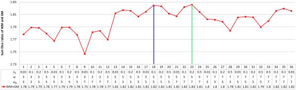
The sum of Dice ratios of WM and GM with respect to the different combinations of the parameters λ₁, w and w_p. The 1^st best and 2^nd best parameters are indicated by the green and blue lines, respectively.

In the following, we explore the relationship between the number of templates and segmentation accuracy. Fig. 8 shows the Dice ratios as a function of different number of templates. As shown in this figure, increasing the number of templates generally improves the segmentation accuracy, as the average Dice ratio increased from 0.87 (N = 1) to 0.92 (N = 19) for WM, and 0.86 (N = 1) to 0.90 (N = 19) for GM. Increasing the number of templates seems to make the segmentations more consistent as reflected by the reduced standard deviation from 0.015 (N = 1) to 0.01 (N = 19) for WM, and 0.012 (N = 1) to 0.004 (N = 19) for GM. Though the experiment shows an increase of accuracy with increasing number of templates, the segmentation performance begins to converge after N = 19. Therefore, in this paper, we choose N = 20, considering the balance of segmentation accuracy and computational efficiency.

Figure 8.

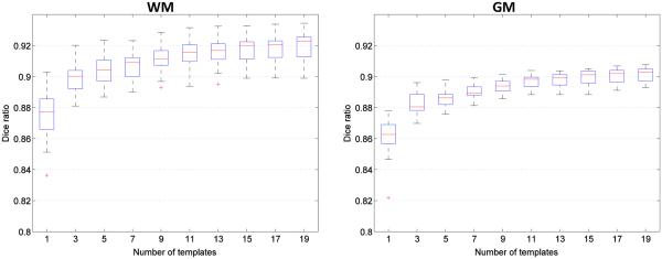
Box-whisker plots of Dice ratio of segmentation using an increasing number of templates from the library. Experiment is performed by leave-one-out strategy on a library of 20 templates.

4.2 Leave-one-out cross validation

To evaluate the performance of the proposed method, we measured the Dice ratio between the automated and ground truth for the 20 template images in a leave-one-out cross-validation fashion, which has been adopted in numerous papers (Aljabar et al., 2009; Coupé et al., 2011; Shi et al., 2009; Wang et al., 2012). In each cross-validation step, 19 images were used as priors and the remaining image was used as the testing image to be segmented by the proposed method. This process was repeated until each image was taken as the testing image once.

Fig. 9 shows the segmentation results of different methods for one typical subject. We first show the results of majority voting (MV) scheme after nonlinear alignment with the testing subject, as shown in Fig. 9(c). We then compare with our previous proposed method, namely the coupled level set (CLS) method (Wang et al., 2011) (the algorithm is publicly available at http://www.nitrc.org/projects/ibeat/), in which the atlas from (Shi et al., 2011b) was utilized to guide the tissue segmentation with the results shown in Fig. 9(d). We also make a comparison with the conventional patch-based method (CPM) (Coupé et al., 2011) with the results shown in Fig. 9(e). Note that, to make a fair comparison, we perform a similar cross-validation as in Section 4.1 to derive the optimal parameters for the CPM, finally obtaining the patch size of 5 × 5 × 5 and the neighborhood size of 5 × 5 × 5. To demonstrate the advantage of using the sparsity, we make a comparison between the subject-specific atlases without and with sparsity constraint, as shown in Fig. 9(f) and (g), respectively. The last two rows in Fig. 9 present the results of the proposed method (Eq. (4)) without and with spatial consistency as introduced in Section 3.3. To better compare the results of different methods, the label differences compared with the ground truth are also presented in Fig. 10, which qualitatively demonstrates the advantage of the proposed method.

Figure 9.

Comparison with different methods. From top to bottom: (a) original images, (b) ground-truth segmentation, (c) results of majority voting (MV), (d) results of the coupled level set (CLS) method (Wang et al., 2011), (e) results of the conventional patch-based method (CPM) (Coupé et al., 2011), (f,g) results of the proposed subject-specific atlas without the sparse constraint (f) and with the sparse constraint (g), (h,i) results of the proposed method without spatial consistency (h) and with spatial consistency (i). The label differences are shown in Fig. 10.

Figure 10.

(a-g) show WM differences between ground-truth segmentations and automated segmentations of different methods; (h-n) show GM differences between ground-truth segmentations and automated segmentations of different methods. Dark red indicates false negative, while dark blue indicates false positive.

In the following, we will quantitatively evaluate the performance of different methods in terms of segmentation accuracy in both global metric (Dice ratio) and local metrics (surface distance and landmark curve distance). Dice ratios of different methods are shown in Fig. 11. It can be seen that the results of the proposed method outperform the majority voting (MV), the coupled level set (CLS) method (Wang et al., 2011) and the conventional patch-based method (CPM) (Coupé et al., 2011) on all subjects. Specifically, the average Dice ratios are 0.822±0.016 (WM) and 0.818±0.015 (GM) by the MV, 0.875±0.014 (WM) and 0.856±0.005 (GM) by the CLS, and are 0.87±0.01 (WM) and 0.863±0.006 (GM) by the CPM, respectively. We also make a comparison with the segmentation obtained by using the subject-specific atlas without and with the sparse constraint as proposed in Section 3.2. The Dice ratios are 0.870±0.01 (WM) and 0.845±0.01 (GM) for the subject-specific atlas without the sparse constraint, while 0.897±0.009 (WM) and 0.869±0.004 (GM) for the subject-specific atlas with the sparse constraint, which clearly demonstrates the advantage of the sparsity in terms of accuracy. We then make a comparison with the proposed method (Eq. (14)) without and with the spatial consistency as introduced in Section 3.3. Without the spatial consistency, the Dice ratios are 0.907±0.009 (WM) and 0.891±0.006 (GM), while, with spatial consistency, the Dice ratios are 0.919±0.008 (WM) and 0.901±0.005 (GM), which demonstrates the importance of the spatial consistency.

Figure 11.

Dice ratios of different methods in cortical regions: majority voting (MV), the coupled level set (CLS) (Wang et al., 2011), the conventional patch-based method (CPM) (Coupé et al., 2011), the proposed subject-specific atlas without and with the sparse constraint, and the proposed method without and with the spatial consistency.

To further validate the proposed method, we also evaluate the accuracy by measuring the surface distance errors (Li et al., 2012) between ground-truth segmentation and the reconstructed WM/GM (inner) surfaces by CLS, CPM, and our proposed method (with spatial consistency). The surface distance errors on a typical subject are shown in Fig. 12. The upper row of Fig. 12 show the surface distances from the surfaces obtained by these methods to the ground-truth surfaces. Since the surface distance measure is not symmetrical, the surface distances from the ground-truth surfaces to the automatically obtained surfaces are also shown in the lower row of the figure. The large surface distance errors on the gyral crest in Fig. 12(d) and (e) reflect that the thin gyral rests are not correctly segmented by CLS and CPM. On the other hand, it can be seen that our proposed method agrees most with the ground truth. The average surface distance errors on 10 subjects are shown in Fig. 13, which again demonstrates the advantage of our proposed method.

Figure 12.

The upper row shows the surface distances in mm from the surfaces obtained by the CLS (Wang et al., 2011) (left), the conventional patch-based method (CPM) (Coupé et al., 2011) (middle) and our proposed method (right) to the ground-truth surfaces. The lower row shows the surface distances from the ground-truth surfaces to the surfaces obtained by three different methods.

Figure 13.

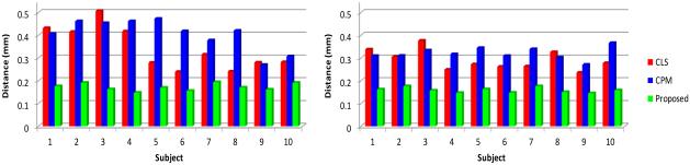
Left: the average surface distances from the surfaces obtained by three different methods to the ground-truth surfaces on 10 subjects; Right: the average surface distances from the ground-truth surfaces to the surfaces by three different methods on 10 subjects.

The above surface distance is measured from each point in one surface to its closest point on the other surface, which, however, tends to under-estimate the errors. For example, ideally, a point on the gyral crest should find a closest point on the gyral crest to measure the distance, while with the above surface distance definition it might incorrectly find the closest point on the sulcal bank. To better reflect the accuracy of the methods on the gyral crests, we further measure the distance of gyral landmark curves on the cortical surfaces. Large curve distance error indicates that the gyral crest is poorly resolved. We selected two major gyri, i.e., the superior temporal gyral curve and the postcentral gyral curve, as the landmarks to measure the accuracy. We manually labeled two sets of gyral curves using the method in (Li et al., 2010) on the inner cortical surfaces from different tissue segmentation results. One typical example is shown in the upper row of Fig. 14, in which the white curves were delineated by the experts on the superior temporal gyrus and postcentral gyrus, and the surfaces are color-coded by the maximum principal curvature (Li et al., 2010). Average symmetric curve distance errors (Li and Shen, 2011) on each curve of 10 subjects are computed, as shown in the upper row of Fig. 15. Compared with CLS and CPM, the proposed method achieves higher accuracy in terms of landmark curves.

Figure 15.

The upper rows are the average symmetric curve distances of three different methods on the superior temporal gyrus and the postcentral gyrus of 10 subjects. The lower rows are the results of average differences of local GI and global GI by three different methods on 10 subjects.

Gyrification index (GI) (Zilles et al., 1988), a metric that quantifies the amount of cortex buried within the sulcal folds as compared with the amount of cortex on the outer visible cortex, has been widely used in measuring brain structural convolution. Unsatisfying segmentation results usually diminish the cortical folding and result into a low GI. Therefore, we also measure local GI (Schaer et al., 2008) and global GI (Zilles et al., 1988) to evaluate the folding complexity of the inner cortical surface. One typical example of the local GI maps (with the radius 25mm) by the three methods are shown in the lower row of Fig. 14. Since some thin gyri in WM by the CLS and CPM were missing, the local GI is relatively lower than the ground truth. The average difference of local and global GI compared to the ground truth on all 10 subjects are plotted in the lower row of Fig. 15. It can be seen that the results by our proposed method show the highest agreement with the ground truth on both local and global GI, indicating that the cortical folding resolved by our method are similar to the ground truth.

4.3 Results on 8 new testing subjects with ground truth

Instead of using the leave-one-out cross-validation fashion, we further validated our proposed method on 8 additional subjects, which were not included in the library. The gestational age of the 8 neonates was 38±1.0 weeks at birth and 43.1±1.6 weeks at MR scanning, using the same imaging parameters as in the template library. For comparison, we use the manual segmentations by experts as reference. These manual segmentation were performed on 1 axial slice, 1 coronal slice, and 1 sagittal slice by using ITK-SNAP software (Yushkevich et al., 2006), as shown in Fig. 16. Note that the subcortical region is unlabeled due to its low contrast. The segmentation results of different methods are shown in Fig. 16(c-e), with WM differences shown in (f-h) and GM differences shown in (i-k). By visual inspection, our proposed method achieves the smallest errors, which is also confirmed by the Dice ratios on 8 subjects as shown in Fig. 17.

Figure 16.

Comparisons of three different methods on a randomly selected subject from 8 additional subjects. From left to right: (a) original images, (b) ground-truth segmentation (which we called ground-truth in the figure), (c) results of the coupled level set (CLS) method (Wang et al., 2011), (d) results of the CPM (Coupé et al., 2011), (e) results of our proposed method, (f-h) WM differences between manual segmentations and automated segmentations by three different methods, (i-k) GM differences between manual segmentations and automated segmentations by three different methods. Dark red indicates false negative, while dark blue indicates false positive.

Figure 17.

Dice ratios for 8 additional subjects by three different segmentation methods in cortical regions.

4.4 Results on 94 testing subjects for qualitative evaluation

The proposed method has also been qualitatively evaluated on 94 additional subjects without ground truth available. The gestational age of the 94 neonates was 38.5±1.7 weeks at birth and 44.1±2.6 weeks at MR scanning. Imaging parameters, as shown in Table 1, are the same as those used in the template library. The segmentation of all subjects were visually inspected by experts, confirming the good quality of the results. Here we randomly show 14 segmentation results from total 94 subjects in Fig. 18. As can be observed, the results of the proposed method demonstrate better segmentation accuracy than those by the coupled level set (CLS) method (Wang et al., 2011) and the conventional patch-based method (CPM) (Coupé et al., 2011), by using the the original intensity images as references.

Table 1.

Scanning protocol parameters: the repetition time (TR), the echo time (TE), the flip angle (FA) ,and the image resolution.

Sequence #	Number of Subjects	Manufacturer	Field Strength	T2 Protocol
				TR(ms)	TE(ms)	FA( °)	Resolution (mm3)
1	122	SIEMENS	3.0 T	7380	119	150	1.25×1.25×1.95
2	10	SIEMENS	3.0 T	9280	119	150	1.0×1.0×1.3
3	10	GE	1.5 T	3500	17	180	1.0×1.0×3.0
4	10	Philips	3.0 T	2500	279	90	1.0×1.0×1.0

Figure 18.

Results of three different methods on 14 subjects. In each panel, the original images and their respective results by the coupled level set (CLS) method (Wang et al., 2011), the conventional patch-based method (CPM) (Coupé et al., 2011), and our proposed method are shown from left to right.

4.5 Evaluation on images with different scanning parameters

In the previous Sections 4.2-4.4, we have shown the segmentation results on subjects scanned using similar imaging parameters as those used for building the template library, as shown in the sequence #1 of Table 1. To demonstrate the robustness and wide applicability of the proposed method, we tested our method on 30 additional images which were acquired on different scanners with different acquisition protocols and parameters, shown as sequence #2, sequence #3 (from NIH Pediatric MRI Data Repository, http://pediatricmri.nih.gov/nihpd/info/index.html), and sequence #4 in Table 1, respectively. Fig. 19 shows 3 randomly selected subjects and their corresponding segmentation results of different methods for each scanning protocol in sequence #2, sequence #3, and sequence #4. The conventional patch-based (CPM) method (Coupé et al., 2011), using the sum of the squared difference (SSD) based similarity measure, is sensitive to the variance in contrast and luminance (see sequence #2 in Fig. 19), although we have performed intensity normalization before running the CPM. The coupled level set (CLS) method (Wang et al., 2011) utilizes the population-based atlas and global intensity information to derive an initialization for the subsequent coupled level sets based segmentation. However, due to the low guidance capability of population-based atlas and the large overlap of the tissue intensity distributions, the CLS cannot achieve a good segmentation neither, as shown in sequence #3 and #4 of Fig. 19, in which most of CSF in the ventricle has been incorrectly labeled as WM. By contrast, our method achieves visually reasonable results for these images with different protocols. We then further calculate the Dice ratios of different methods by comparing to the manual segmentation results shown in Fig. 20, which again demonstrates that our method achieves the highest accuracy. The robustness of our method on images acquired with different protocols may come from following aspects: First, our method works on image patches, where similar local patterns can be captured although the whole images may have large contrast differences. Second, all the patches are normalized to have the unit ℓ-norm to alleviate the intensity scale problem (Cheng et al., 2009; Wright et al., 2010). Third, the testing patch is well represented by the over-complete patch dictionary with the sparsity constraint. The derived sparse coefficients are utilized to (1) measure the patch similarity, instead of directly using the intensity difference similarity as used SSD in the CPM (Coupé et al., 2011), and (2) estimate a subject-specific atlas, instead of a population-based atlas as used in CLS (Wang et al., 2011).

Figure 19.

Segmentation results of different methods on images acquired on different scanners and protocols, which demonstrate the robustness and wide applicability of our method. The imaging parameters for the images from top to bottom are listed in sequence #2, sequence #3, and sequence #4 of Table 1, respectively.

Figure 20.

Dice ratios of three different segmentation methods on the images acquired with different protocols.

4.6 Computational time

The average total computational time is around 120 mins for the segmentation of a 256×256×198 image with a spatial resolution of 1×1×1 mm³ on our linux server with 8 CPUs and 16G memory. In this computational time, on average, it takes around 30 mins to derive the subject-specific atlas and 50 mins to enforce the spatial consistency and derive the final level set segmentation. The rest of the time is consumed by preprocessing and linearly aligning the library template images onto the to-be-segmented testing subject. Overall, the proposed method is able to achieve satisfactory segmentation results within a reasonable computational time.

5. Discussion and conclusion

In our previous method (Wang et al., 2013), we proposed to segment neonatal images by utilizing the additional knowledge from their specific follow-up images. The Dice ratios for WM and GM of this method are 0.94±0.01 and 0.92±0.01, respectively. However, this method requires the availability of follow-up scans and thus limits its usage. Given that many neonatal subjects do not have longitudinal follow-up scans or cannot wait for such a long time for image processing, the proposed method is standalone on the neonatal images and achieves quite competing results with Dice ratios 0.92±0.01 (WM) and 0.90±0.01 (GM) in the cortical regions.

It is well known that manual segmentation is a difficult, tedious, and very time consuming task. Due to the extremely low tissue contrast, it becomes much more difficult to perform the manual segmentation in the subcortical region, even for an experienced expert. Therefore, in all our evaluations, we only focus on comparing the segmentations in the cortical regions with the manual segmentations by excluding the subcortical region. Although the segmentation in the subcortical regions are not quantitatively evaluated, the proposed method achieves visually reasonable segmentation results.

In neonates, the myelinated WM is mainly located in the subcortical regions. However, in our current work, we segment a brain image into general GM, WM, and CSF, in which WM contains both myelinated and unmyelinated WM. In our future work, we will separate myelinated WM from unmyelinated WM by considering multi-modality information (Gui et al., 2012).

In summary, we have proposed a novel patch-driven level sets method for neonatal brain MR image segmentation. A subject-specific atlas was first built from the template library. The spatial consistency in the probability maps from the subject-specific atlas was then enforced by considering the similarities of a patch with its neighboring patches. The final segmentation was derived by integration of the subject-specific atlas into a level set segmentation framework. The proposed method has been extensively evaluated on 20 training subjects using leave-one-out cross-validation, and also on 8 additional testing subjects with ground truth and 94 subjects without ground truth, showing very promising results compared with state-of-the-art methods. Further evaluation of our method showed robustness and applicability in the segmentation of images acquired from different scanners using different acquisition protocols and parameters.

Research highlight.

• ▶ A patch-driven level-sets based neonatal image segmentation method is proposed.

• ▶ A subject-specific atlas is built from a library by using sparse representation.

• ▶ The spatial consistency in the probability maps is further enforced.

• ▶ The subject-specific atlas is integrated into a coupled level set framework.

• ▶ The proposed method has been extensively evaluated on 152 subjects.

Figure 14.

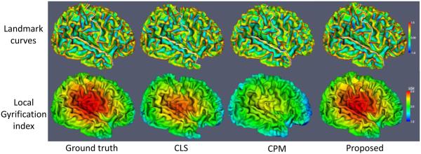
The upper row shows the manually labeled postcentral and superior temporal gyral landmark curves, while the lower row shows the results of local gyrification index by three different methods.

Appendix 1

$$\begin{array}{cc}\hfill & E^{LGD\_Prior}\left(C\right)=-\underset{j}{\Sigma }\underset{x\in {\Omega }_j}{\Sigma }\log P_j^{LGD\_Prior}\left(x\right)\hfill \\ \hfill & =\underset{j}{\Sigma }\underset{x\in {\Omega }_j}{\Sigma }\left\{-\log \frac{1}{\left|\mathcal{N}\left(x\right)\right|}\underset{y\in \mathcal{N}\left(x\right)}{\Sigma }{P}_j\left(x\right)p_{j,y}\left(I\left(x\right)\right)-\log \left|\mathcal{N}\left(x\right)\right|+\log Z_1\left(x\right)\right\}\hfill \\ \hfill & =\underset{j}{\Sigma }\underset{x\in {\Omega }_j}{\Sigma }\left\{-\log \frac{1}{\left|\mathcal{N}\left(x\right)\right|}\underset{y\in \mathcal{N}\left(x\right)}{\Sigma }{P}_j\left(x\right)p_{j,y}\left(I\left(x\right)\right)\right\}-\underset{j}{\Sigma }\underset{x\in {\Omega }_j}{\Sigma }\log \left|\mathcal{N}\left(x\right)\right|+\underset{x\in \Omega }{\Sigma }\log Z_1\left(x\right)\hfill \end{array}$$

Since the second term −∑_j ∑_z∈Ωj log |𝒩(x)| is a constant and the last term Σ_x∈Ω log Z₁(x) is independent of the choice of partitions Ω_j, the last two terms can be omitted. Thus, we only need to minimize the first term ${\Sigma }_i{\Sigma }_{x\in {\Omega }_j}\left\{-\log \frac{1}{\left|\mathcal{N}\left(x\right)\right|}{\Sigma }_{y\in \mathcal{N}\left(x\right)}{P}_j\left(x\right)p_{j,y}\left(I\left(x\right)\right)\right\}$. Since −log is a convex function, based on Jensen’s inequality, we can derive,

$$\underset{j}{\Sigma }\underset{x\in {\Omega }_j}{\Sigma }\left\{-\log \frac{1}{\left|\mathcal{N}\left(x\right)\right|}\underset{y\in \mathcal{N}\left(x\right)}{\Sigma }{P}_j\left(x\right)p_{j,y}\left(I\left(x\right)\right)\right\}\le \underset{j}{\Sigma }\underset{x\in {\Omega }_j}{\Sigma }\left\{-\frac{1}{\left|\mathcal{N}\left(x\right)\right|}\underset{y\in \mathcal{N}\left(x\right)}{\Sigma }\log \left(P_j\left(x\right)p_{j,y}\left(I\left(x\right)\right)\right)\right\}$$

Therefore, we can simply minimize the right part energy functional in order to minimize E^lgd_prior (C). Note that the right part energy functional is the exact energy functional in the (Wang et al., 2011; Wang et al., 2013), which is much easier to minimize since the logarithm transformation will eliminate the exponential form.

Appendix 2

Based on Appendix 1, we can derive,

$$-\underset{j}{\Sigma }\underset{x\in M_j\left(\Phi \right)}{\Sigma }\log \left\{\frac{1}{Z}\underset{y\in \mathcal{N}\left(x\right)}{\Sigma }{\alpha }_y^{\prime }{P}_j\left(x\right)p_{j,y}\left(I\left(x\right)\right)\right\}\le -\underset{j}{\Sigma }\underset{x\in M_j\left(\Phi \right)}{\Sigma }\left\{\frac{1}{Z}\underset{y\in \mathcal{N}\left(x\right)}{\Sigma }{\alpha }_y\log \left\{P_j\left(x\right)p_{j,y}\left(I\left(x\right)\right)\right\}\right\}$$ (15)

where $Z={\Sigma }_{y\in \mathcal{N}\left(x\right)}{\alpha }_y^{\prime }$. Therefore, we can minimize the right part energy functional, denoted by Ẽ^{patch_LGD_Prior} (Φ), in order to minimize the left one. For convenience of computation, we further replace 𝒩 (x) by a truncated Gaussian kernel K_σ with the scale σ to control the size of the neighborhood (Li et al., 2007, 2008). Finally, we derive the following energy functional,

$$\begin{array}{cc}\hfill & {\tilde{E}}^{Patch\_LGD\_Prior}\left(\Phi \right)\hfill \\ \hfill =-\underset{j}{\Sigma }\underset{x}{\Sigma }\underset{y}{\Sigma }& \frac{1}{Z}{K}_{\sigma }(y-x){\alpha }_y\log \left\{P_j\left(x\right)p_{j,y}\left(I\left(x\right)\right)\right\}{M}_j\left(\Phi \left(x\right)\right)\hfill \end{array}$$ (16)

Note that the second term in Eq. (14) is independent of Φ, and thus it can be omitted. Therefore, minimization of the energy functional in Eq. (14) can be converted to minimization of the following energy functional,

$$E\left(\Phi \right)={\tilde{E}}^{Patch\_LGD\_Prior}\left(\Phi \right)+\beta (E_{{\Phi }_1}+E_{{\Phi }_1})+\nu R\left(\Phi \right)$$ (17)

By calculus of variations, minimization of the energy functional in Eq. (17) with respect to ø₁, ø₂ and ø₃ is achieved by solving the gradient descent flow equations as follows,

$$\begin{array}{cc}\hfill & \frac{\partial {\varphi }_1}{\partial t}=-\delta \left({\varphi }_1\right)\left\{H\left({\varphi }_2\right)(e_1-e_2)H\left({\varphi }_3\right)-\nu \mathrm{div}\left(\frac{\nabla {\varphi }_1}{|\nabla {\varphi }_1|}\right)+\beta [1-(H({\varphi }_2-d_1)-H({\varphi }_2-d_2))][2H\left({\varphi }_1\right)-H({\varphi }_2-d_1)-H({\varphi }_2-d_2)]\right\}\hfill \\ \hfill & \frac{\partial {\varphi }_2}{\partial t}=-\delta \left({\varphi }_2\right)\left\{(H\left({\varphi }_1\right)(e_1-e_2)+(e_2-e_3))H\left({\varphi }_3\right)-\nu \mathrm{div}\left(\frac{\nabla {\varphi }_2}{|\nabla {\varphi }_2|}\right)+\beta [1-(H({\varphi }_1+d_2)-H({\varphi }_1+d_1))][2H\left({\varphi }_2\right)-H({\varphi }_1+d_1)-H({\varphi }_1+d_2)]\right\}\hfill \\ \hfill & \frac{\partial {\varphi }_3}{\partial t}=-\delta \left({\varphi }_3\right)\left\{H\left({\varphi }_1\right)H\left({\varphi }_2\right)e_1+(1-H\left({\varphi }_1\right))H\left({\varphi }_2\right)e_2+(1-H\left({\varphi }_2\right))e_3-e_4-\nu \mathrm{div}\left(\frac{\nabla {\varphi }_3}{|\nabla {\varphi }_3|}\right)\right\}\hfill \end{array}$$

where δ is the Delta function and $e_j\left(x\right)=-{\Sigma }_y\frac{1}{Z}{K}_{\sigma }(y-x){\alpha }_y\log P_j\left(x\right)+{\Sigma }_y\frac{1}{Z}{K}_{\sigma }(y-x){\alpha }_y\left[\log {\sigma }_j\left(y\right)+\frac{{(u_j\left(y\right)-I\left(x\right))}^2}{2{\sigma }_j^2\left(y\right)}\right]$.

References

- Aljabar P, Heckemann RA, Hammers A, Hajnal JV, Rueckert D. Multi-atlas based segmentation of brain images: Atlas selection and its effect on accuracy. NeuroImage. 2009;46:726–738. doi: 10.1016/j.neuroimage.2009.02.018. [DOI] [PubMed] [Google Scholar]
- Anbeek P, Vincken K, Groenendaal F, Koeman A, VAN Osch M, VAN DER Grond J. Probabilistic Brain Tissue Segmentation in Neonatal Magnetic Resonance Imaging. Pediatr Res. 2008;63:158–163. doi: 10.1203/PDR.0b013e31815ed071. [DOI] [PubMed] [Google Scholar]
- Ashburner J, Friston KJ. Unified segmentation. NeuroImage. 2005;26:839–851. doi: 10.1016/j.neuroimage.2005.02.018. [DOI] [PubMed] [Google Scholar]
- Asman AJ, Landman BA. Non-local statistical label fusion for multi-atlas segmentation. Medical Image Analysis. 2012 doi: 10.1016/j.media.2012.10.002. [DOI] [PMC free article] [PubMed] [Google Scholar]
- Bhatia KK, Hajnal JV, Puri BK, Edwards AD, Rueckert D. Consistent Groupwise Non-Rigid Registration for Atlas Construction. ISBI. IEEE. 2004:908–911. [Google Scholar]
- Buades A, Coll B, Morel JM. A non-local algorithm for image denoising. Computer Vision and Pattern Recognition, 2005. CVPR 2005. IEEE Computer Society Conference on. 2005;62:60–65. [Google Scholar]
- Chan TF, Vese LA. Active contours without edges; IEEE Trans Med Imaging 10; 2001. pp. 266–277. [DOI] [PubMed] [Google Scholar]
- Cheng H, Liu Z, Yang L. Sparsity induced similarity measure for label propagation; Computer Vision, 2009 IEEE 12th International Conference on; 2009. pp. 317–324. [Google Scholar]
- Cocosco CA, Zijdenbos AP, Evans AC. A fully automatic and robust brain MRI tissue classification method. Medical Image Analysis. 2003a;7:513–527. doi: 10.1016/s1361-8415(03)00037-9. [DOI] [PubMed] [Google Scholar]
- Cocosco CA, Zijdenbos AP, Evans AC. A fully automatic and robust brain MRI tissue classification method. Med Image Anal. 2003b;7:513–527. doi: 10.1016/s1361-8415(03)00037-9. [DOI] [PubMed] [Google Scholar]
- Coupé P, Eskildsen SF, Manjón JV, Fonov V, Collins DL. Simultaneous segmentation and grading of anatomical structures for patient's classification: Application to Alzheimer's disease. NeuroImage. 2012a;59:3736–3747. doi: 10.1016/j.neuroimage.2011.10.080. [DOI] [PubMed] [Google Scholar]
- Coupé P, Eskildsen SF, Manjón JV, Fonov VS, Pruessner JC, Allard M, Collins DL. Scoring by nonlocal image patch estimator for early detection of Alzheimer's disease. NeuroImage: Clinical. 2012b;1:141–152. doi: 10.1016/j.nicl.2012.10.002. [DOI] [PMC free article] [PubMed] [Google Scholar]
- Coupé P, Manjón J, Fonov V, Pruessner J, Robles M, Collins DL. Patch-based segmentation using expert priors: Application to hippocampus and ventricle segmentation. NeuroImage. 2011;54:940–954. doi: 10.1016/j.neuroimage.2010.09.018. [DOI] [PubMed] [Google Scholar]
- Dempster AP, Laird NM, Rubin DB. Maximum likelihood from incomplete data via the EM algorithm. (B).Journal of the Royal Statistical Society. 1977;39:1–38. [Google Scholar]
- Efron B, Hastie T, Johnstone I, Tibshirani R. Least angle regression. Annals of Statistics. 2004;32:407–499. [Google Scholar]
- Elad M, Aharon M. Image Denoising Via Sparse and Redundant Representations Over Learned Dictionaries. Image Processing, IEEE Transactions on. 2006;15:3736–3745. doi: 10.1109/tip.2006.881969. [DOI] [PubMed] [Google Scholar]
- Ericsson A, Aljabar P, Rueckert D. Construction of a patient-specific atlas of the brain: Application to normal aging; Biomedical Imaging: From Nano to Macro, 2008. ISBI 2008. 5th IEEE International Symposium on; 2008. pp. 480–483. [Google Scholar]
- Eskildsen SF, Coupé P, Fonov V, Manjón JV, Leung KK, Guizard N, Wassef SN, Østergaard LR, Collins DL. BEaST: Brain extraction based on nonlocal segmentation technique. NeuroImage. 2012;59:2362–2373. doi: 10.1016/j.neuroimage.2011.09.012. [DOI] [PubMed] [Google Scholar]
- Fadili MJ, Starck JL, Murtagh F. Inpainting and Zooming Using Sparse Representations. The Computer Journal. 2009;52:64–79. [Google Scholar]
- Fischl B, Dale A. Measuring the Thickness of the Human Cerebral Cortex from Magnetic Resonance Images. Proceedings of the National Academy of Sciences. 2000;97:11044–11049. doi: 10.1073/pnas.200033797. [DOI] [PMC free article] [PubMed] [Google Scholar]
- Fischl B, Salat DH, Busa E, Albert M, Dieterich M, Haselgrove C, van der Kouwe A, Killiany R, Kennedy D, Klaveness S, Montillo A, Makris N, Rosen B, Dale AM. Whole Brain Segmentation: Automated Labeling of Neuroanatomical Structures in the Human Brain. Neuron. 2002;33:341–355. doi: 10.1016/s0896-6273(02)00569-x. [DOI] [PubMed] [Google Scholar]
- Gao Y, Liao S, Shen D. Prostate segmentation by sparse representation based classification. Medical Physics. 2012;39:6372–6387. doi: 10.1118/1.4754304. [DOI] [PMC free article] [PubMed] [Google Scholar]
- Geffroy D, Goldenberg R, Kimmel R, Rivlin E, Rudzsky M. Cortex Segmentation: A Fast Variational Geometric Approach. IEEE Trans Med Imaging. 2002;21:1544–1551. doi: 10.1109/TMI.2002.806594. [DOI] [PubMed] [Google Scholar]
- Gui L, Lisowski R, Faundez T, Hüppi PS, Lazeyras F.o., Kocher M. Morphology-driven automatic segmentation of MR images of the neonatal brain. Med Image Anal. 2012;16:1565–1579. doi: 10.1016/j.media.2012.07.006. [DOI] [PubMed] [Google Scholar]
- Han X, Pham DL, Tosun D, Rettmann ME, Xu C, Prince JL. CRUISE: Cortical reconstruction using implicit surface evolution. NeuroImage. 2004;23:997–1012. doi: 10.1016/j.neuroimage.2004.06.043. [DOI] [PubMed] [Google Scholar]
- Kuklisova-Murgasova M, Aljabar P, Srinivasan L, Counsell SJ, Doria V, Serag A, Gousias IS, Boardman JP, Rutherford MA, Edwards AD, Hajnal JV, Rueckert D. A dynamic 4D probabilistic atlas of the developing brain. NeuroImage. 2011;54:2750–2763. doi: 10.1016/j.neuroimage.2010.10.019. [DOI] [PubMed] [Google Scholar]
- Langerak TR, van der Heide UA, Kotte ANTJ, Viergever MA, van Vulpen M, Pluim JPW. Label Fusion in Atlas-Based Segmentation Using a Selective and Iterative Method for Performance Level Estimation (SIMPLE) Medical Imaging, IEEE Transactions on. 2010;29:2000–2008. doi: 10.1109/TMI.2010.2057442. [DOI] [PubMed] [Google Scholar]
- Leroy F, Mangin J, Rousseau F, Glasel H, Hertz-Pannier L, Dubois J, Dehaene-Lambertz G. Atlas-free surface reconstruction of the cortical grey-white interface in infants. PLoS One. 2011;6:e27128. doi: 10.1371/journal.pone.0027128. [DOI] [PMC free article] [PubMed] [Google Scholar]
- Li CM, Kao CY, Gore JC, Ding ZH. Implicit Active Contours Driven by Local Binary Fitting Energy; CVPR; 2007. pp. 1–7. [Google Scholar]
- Li CM, Kao CY, Gore JC, Ding ZH. Minimization of Region-Scalable Fitting Energy for Image Segmentation. TIP. 2008;17:1940–1949. doi: 10.1109/TIP.2008.2002304. [DOI] [PMC free article] [PubMed] [Google Scholar]
- Li G, Guo L, Nie J, Liu T. An automated pipeline for cortical sulcal fundi extraction. Med Image Anal. 2010;14:343–359. doi: 10.1016/j.media.2010.01.005. [DOI] [PMC free article] [PubMed] [Google Scholar]
- Li G, Nie J, Wang L, Shi F, Lin W, Gilmore JH, Shen D. Mapping Region-Specific Longitudinal Cortical Surface Expansion from Birth to 2 Years of Age. Cerebral Cortex. 2012 doi: 10.1093/cercor/bhs265. [DOI] [PMC free article] [PubMed] [Google Scholar]
- Li G, Shen D. Consistent sulcal parcellation of longitudinal cortical surfaces. NeuroImage. 2011;57:76–88. doi: 10.1016/j.neuroimage.2011.03.064. [DOI] [PMC free article] [PubMed] [Google Scholar]
- Mairal J, Bach F, Ponce J, Sapiro G, Zisserman A. Discriminative learned dictionaries for local image analysis; Computer Vision and Pattern Recognition, 2008. CVPR 2008. IEEE Conference on; 2008a. pp. 1–8. [Google Scholar]
- Mairal J, Elad M, Sapiro G. Sparse Representation for Color Image Restoration. Image Processing, IEEE Transactions on. 2008b;17:53–69. doi: 10.1109/tip.2007.911828. [DOI] [PubMed] [Google Scholar]
- Merisaari H, Parkkola R, Alhoniemi E, Ter?s M, Lehtonen L, Haataja L, Lapinleimu H, Nevalainen OS. Gaussian mixture model-based segmentation of MR images taken from premature infant brains. Journal of Neuroscience Methods. 2009;182:110–122. doi: 10.1016/j.jneumeth.2009.05.026. [DOI] [PubMed] [Google Scholar]
- Mewes AUJ, Huppi PS, Als H, Rybicki FJ, Inder TE, McAnulty GB, Mulkern RV, Robertson RL, Rivkin MJ, Warfield SK. Regional brain development in serial magnetic resonance imaging of low-risk preterm infants. Pediatrics. 2006;118:23–33. doi: 10.1542/peds.2005-2675. [DOI] [PubMed] [Google Scholar]
- Prastawa M, Gilmore JH, Lin W, Gerig G. Automatic segmentation of MR images of the developing newborn brain. Med Image Anal. 2005;9:457–466. doi: 10.1016/j.media.2005.05.007. [DOI] [PubMed] [Google Scholar]
- Rousseau F, Habas PA, Studholme C. A Supervised Patch-Based Approach for Human Brain Labeling. TMI. 2011;30:1852–1862. doi: 10.1109/TMI.2011.2156806. [DOI] [PMC free article] [PubMed] [Google Scholar]
- Sabuncu MR, Yeo BTT, Van Leemput K, Fischl B, Golland P. A Generative Model for Image Segmentation Based on Label Fusion. Medical Imaging, IEEE Transactions on. 2010;29:1714–1729. doi: 10.1109/TMI.2010.2050897. [DOI] [PMC free article] [PubMed] [Google Scholar]
- Schaer M, Cuadra MB, Tamarit L, Lazeyras F, Eliez S, Thiran JP. A surface-based approach to quantify local cortical gyrification. IEEE Trans Med Imaging. 2008;27:161–170. doi: 10.1109/TMI.2007.903576. [DOI] [PubMed] [Google Scholar]
- Shattuck DW, Leahy RM. BrainSuite: an automated cortical surface identification tool. Med Image Anal. 2002;6:129–142. doi: 10.1016/s1361-8415(02)00054-3. [DOI] [PubMed] [Google Scholar]
- Shi F, Fan Y, Tang S, Gilmore JH, Lin W, Shen D. Neonatal Brain Image Segmentation in Longitudinal MRI Studies. NeuroImage. 2009;49:391–400. doi: 10.1016/j.neuroimage.2009.07.066. [DOI] [PMC free article] [PubMed] [Google Scholar]
- Shi F, Shen D, Yap P, Fan Y, Cheng J, An H, Wald LL, Gerig G, Gilmore JH, Lin W. CENTS: cortical enhanced neonatal tissue segmentation. Hum Brain Mapp. 2011a;32:382–396. doi: 10.1002/hbm.21023. [DOI] [PMC free article] [PubMed] [Google Scholar]
- Shi F, Wang L, Dai Y, Gilmore JH, Lin W, Shen D. Pediatric Brain Extraction Using Learning-based Meta-algorithm. NeuroImage. 2012;62:1975–1986. doi: 10.1016/j.neuroimage.2012.05.042. [DOI] [PMC free article] [PubMed] [Google Scholar]
- Shi F, Yap P, Fan Y, Gilmore JH, Lin W, Shen D. Construction of Multi-Region-Multi-Reference Atlases for Neonatal Brain MRI Segmentation. NeuroImage. 2010;51:684–693. doi: 10.1016/j.neuroimage.2010.02.025. [DOI] [PMC free article] [PubMed] [Google Scholar]
- Shi F, Yap P, Wu G, Jia H, Gilmore JH, Lin W, Shen D. Infant brain atlases from neonates to 1- and 2-year-olds. PLoS One. 2011b;6:e18746. doi: 10.1371/journal.pone.0018746. [DOI] [PMC free article] [PubMed] [Google Scholar]
- Sled JG, Zijdenbos AP, Evans AC. A nonparametric method for automatic correction of intensity nonuniformity in MRI data. IEEE Trans Med Imaging. 1998;17:87–97. doi: 10.1109/42.668698. [DOI] [PubMed] [Google Scholar]
- Song Z, Awate SP, Licht DJ, Gee JC. Clinical neonatal brain MRI segmentation using adaptive nonparametric data models and intensity-based Markov priors., Med Image Comput Comput Assist Interv Int Conf Med Image Comput Comput Assist Interv. 2007:883–890. doi: 10.1007/978-3-540-75757-3_107. [DOI] [PubMed] [Google Scholar]
- Tibshirani RJ. Regression Shrinkage and Selection via the Lasso. (Series B).Journal of the Royal Statistical Society. 1996;58:267–288. [Google Scholar]
- Wang H, Suh JW, Das SR, Pluta J, Craige C, Yushkevich PA. Multi-Atlas Segmentation with Joint Label Fusion. IEEE Trans. on PAMI. 2012 doi: 10.1109/TPAMI.2012.143. [DOI] [PMC free article] [PubMed] [Google Scholar]
- Wang L, He L, Mishra A, Li C. Active contours driven by local Gaussian distribution fitting energy. Signal Processing. 2009;89:2435–2447. [Google Scholar]
- Wang L, Shi F, Lin W, Gilmore JH, Shen D. Automatic segmentation of neonatal images using convex optimization and coupled level sets. NeuroImage. 2011;58:805–817. doi: 10.1016/j.neuroimage.2011.06.064. [DOI] [PMC free article] [PubMed] [Google Scholar]
- Wang L, Shi F, Yap P, Lin W, Gilmore JH, Shen D. Longitudinally guided level sets for consistent tissue segmentation of neonates. Hum Brain Mapp. 2013;34:956–972. doi: 10.1002/hbm.21486. [DOI] [PMC free article] [PubMed] [Google Scholar]
- Warfield SK, Kaus M, Jolesz FA, Kikinis R. Adaptive, template moderated, spatially varying statistical classification. Med Image Anal. 2000;4:43–55. doi: 10.1016/s1361-8415(00)00003-7. [DOI] [PubMed] [Google Scholar]
- Warfield SK, Zou KH, Wells WM. Simultaneous truth and performance level estimation (STAPLE): an algorithm for the validation of image segmentation. Medical Imaging, IEEE Transactions on. 2004;23:903–921. doi: 10.1109/TMI.2004.828354. [DOI] [PMC free article] [PubMed] [Google Scholar]
- Weisenfeld NI, Mewes AUJ, Warfield SK. Segmentation of newborn brain MRI. ISBI. 2006:766–769. [Google Scholar]
- Weisenfeld NI, Warfield SK. Automatic segmentation of newborn brain MRI. NeuroImage. 2009;47:564–572. doi: 10.1016/j.neuroimage.2009.04.068. [DOI] [PMC free article] [PubMed] [Google Scholar]
- Winn J, Criminisi A, Minka T. Object categorization by learned universal visual dictionary. Tenth IEEE International Conference on Computer Vision. 2005;1802:1800–1807. [Google Scholar]
- Wright J, Yi M, Mairal J, Sapiro G, Huang TS, Shuicheng Y. Sparse Representation for Computer Vision and Pattern Recognition. Proceedings of the IEEE. 2010;98:1031–1044. [Google Scholar]
- Xue H, Srinivasan L, Jiang S, Rutherford M, Edwards AD, Rueckert D, Hajnal JV. Automatic segmentation and reconstruction of the cortex from neonatal MRI. NeuroImage. 2007;38:461–477. doi: 10.1016/j.neuroimage.2007.07.030. [DOI] [PubMed] [Google Scholar]
- Yang J, Wright J, Huang TS, Ma Y. Image Super-Resolution Via Sparse Representation. Image Processing, IEEE Transactions on. 2010;19:2861–2873. doi: 10.1109/TIP.2010.2050625. [DOI] [PubMed] [Google Scholar]
- Yushkevich PA, Piven J, Hazlett HC, Smith RG, Ho S, Gee JC, Gerig G. User-guided 3D active contour segmentation of anatomical structures: Significantly improved efficiency and reliability. NeuroImage. 2006;31:1116–1128. doi: 10.1016/j.neuroimage.2006.01.015. [DOI] [PubMed] [Google Scholar]
- Zeng X, Staib LH, Schultz RT, Duncan JS. Segmentation and Measurement of the Cortex from 3D MR Images Using Coupled Surfaces Propagation. IEEE Trans Med Imaging. 1999;18:927–937. doi: 10.1109/42.811276. [DOI] [PubMed] [Google Scholar]
- Zhang Y, Brady M, Smith S. Segmentation of brain MR images through a hidden Markov random field model and the expectation maximization algorithm. IEEE Trans Med Imaging. 2001;20:45–57. doi: 10.1109/42.906424. [DOI] [PubMed] [Google Scholar]
- Zilles K, Armstrong E, Schleicher A, Kretschmann HJ. The human pattern of gyrification in the cerebral cortex. Anat Embryol (Berl) 1988;179:173–179. doi: 10.1007/BF00304699. [DOI] [PubMed] [Google Scholar]
- Zou H, Hastie T. Regularization and variable selection via the Elastic Net. (Series B).Journal of the Royal Statistical Society. 2005;67:301–320. [Google Scholar]