A Score-Statistic Approach for the Mapping of Quantitative-Trait Loci with Sibships of Arbitrary Size

Abstract

The Haseman-Elston method is widely used for the mapping of quantitative-trait loci. However, this method does not use all the information in the data, because it only considers the sib-pair trait-value difference. In addition, the Haseman-Elston method was developed for independent sib pairs; its generalization to nonindependent sib pairs is not straightforward. Here we introduce a score test statistic derived from a normal likelihood based on multiplex sibship data, conditional on identical-by-descent sharing statuses. This score test is asymptotically equivalent to the corresponding likelihood-ratio test, but it is much easier to implement. Because the proposed test uses all of the trait values, it makes more efficient use of the data than does the Haseman-Elston method. The proposed test is naturally applicable to sibships of arbitrary size. The finite-sample properties of the proposed score statistic are evaluated via simulations.

Introduction

The Haseman-Elston method (H-E method; Haseman and Elston ¹⁹⁷²) has been widely used for the mapping of quantitative-trait loci. This method was originally developed for independent sib pairs. It regresses the squared difference in the trait values of the sib pairs on their estimated proportion of marker alleles that are shared identical by descent (IBD). If the slope of the regression line is significantly less than 0, then there is evidence for linkage between the marker and a trait locus.

However, the squared trait-value difference does not summarize all of the information in the trait data, since the trait data for a sib pair is bivariate in nature (Wright 1997). Recently, regression methods that use other transformations of the trait values as dependent variables have been proposed, to make more efficient use of the trait information (Elston et al. 2000; Xu et al. ²⁰⁰⁰; Forrest ²⁰⁰¹; Sham and Purcell ²⁰⁰¹; Wang et al. ²⁰⁰¹). Similar to the H-E method, these recent modifications were also developed for independent sib-pair data. The use of these methods for dependent sib pairs that arise from multiplex sibships is not straightforward. Generalization of the H-E method to arbitrary sibship size has attracted much interest in the literature. For instance, one way of dealing with a sibship containing more than two sibs is to treat the distinct sib pairs in the sibship as independent and apply the H-E method (Amos et al. 1989; Collins and Morton ¹⁹⁹⁵). To take into account the dependence among the distinct sib pairs from the same sibship, it has been suggested either to adjust the degrees of freedom of the t test statistic (Wilson and Elston 1993) or to use the generalized linear regression technique (Elston et al. 2000).

To make efficient use of the information contained in the trait data, the maximum-likelihood method has also been used for the mapping of quantitative-trait loci (Kruglyak and Lander 1995; Fulker and Cherny ¹⁹⁹⁶; Wright ¹⁹⁹⁷). Because this approach does not require preliminary data reduction, as the H-E method does, it is more powerful when the normality assumption is satisfied. Another advantage of the maximum-likelihood method is that it handles sibships of arbitrary size in a systematic manner. However, implementing the maximum likelihood method involves intensive computation in maximizing the likelihood function. Actually, for large sibships, even the computation of the likelihood function could be very computation intensive, because calculating the likelihood function requires the joint probabilities of the IBD-sharing statuses among all of the sibs. This is a daunting requirement when one considers that the calculation of the IBD-sharing probability even for sib pairs is not trivial (see reports by Kruglyak and Lander [1995], Almasy and Blangero [1998], and Tiwari and Elston [1997], for algorithms for calculating the IBD-sharing probability for sib pairs.)

Therefore, it is desirable to have a test statistic that has the optimal property of the maximum-likelihood method yet is easy to compute. In the present study, we derive a score statistic based on the likelihood function of nuclear families with arbitrary sibship size. This score statistic is asymptotically equivalent to the likelihood-ratio test statistic that corresponds to the maximum-likelihood method. The limiting distribution of this score statistic is derived. This score statistic is easy to compute and directly applies to sibships of arbitrary size. A simulation study is conducted to investigate the type I error rate and the power of this score statistic, which are also compared with those of H-E method.

Methods

Consider n nuclear families with sibship size n_i in the ith family. At any location on the genome, each sib pair can share 0, 1, or 2 alleles IBD. Let π_ikl be the number of marker alleles shared IBD by the kth sib and the lth sib in the ith family. π_ikl is a random variable with possible values of 0, 1, or 2. The probability that π_ikl=0, 1, or 2 between sib pairs can be estimated from the marker data (Fulker et al. 1995; Kruglyak and Lander ¹⁹⁹⁵).

For a sibship of size n_i, there are n_i(n_i-1)/2 distinct sib pairs. Since each sib pair could share 0, 1, or 2 marker alleles IBD, the total number of IBD-sharing configurations for all of these sib pairs is 3^n_i(n_i-1)/2. We denote this number by J_i. Let γ_ij be the probability of the jth configuration for the ith family. This probability can be 0 for some configurations; for instance, in a sibship of size 3, any configuration in which the first sib shares 2 alleles IBD with both the second sib and the third sib, and the second sib and the third sib share 1 allele IBD, has zero probability.

In the same sibship, the IBD-sharing status for one sib pair is independent of that for another sib pair, even when these two sib pairs have one sib in common (Amos et al. 1989). However, the IBD-sharing statuses among all the sib pairs are not jointly independent. This means that γ_ij is not the product of the probabilities of the sib-pair IBD-sharing statuses involved in the jth IBD-sharing configuration. Generally, the following relationship holds:

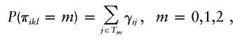where T_m is the set of IBD-sharing configurations in which the kth sib and the lth sib share m alleles IBD.

Let y_i=(y_i1,…,y_ini)^t be a vector consisting of the trait values of the sibs in the ith family. We assume that, given the jth IBD-sharing configuration, the density function of y_i is φ(0,Σ_ij), where

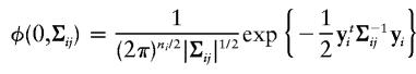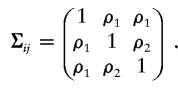
is a multivariate normal density function, and Σ_ij=(σ_kl), with σ_kl=1 if k=l and σ_kl=ρ_m if k≠l, where ρ_m is the correlation coefficient between the kth sib and the lth sib, given that they share m alleles IBD, where m=0,1,2. To see an example of the matrix Σ_ij, consider a sibship of size 3. In this sibship, the matrix Σ_ij that corresponds to a configuration in which sibs 1 and 2 share 1 allele IBD, sibs 1 and 3 share 1 allele IBD, and sibs 2 and 3 share 2 alleles IBD, is

We note that we have assumed that the y_i vectors have been standardized such that each component of y_i has a mean of 0 and a variance of 1. For a discussion about the ways of standardizing y_i vectors, see the Data Standardization section.

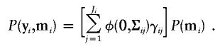
Let m_i denote the marker data in the ith family. Since there are J_i IBD-sharing configuration patterns among the n_i sibs in the ith family, the probability of (y_i,m_i) is

The unknown parameters in the above equation are ρ₀, ρ₁, and ρ₂. The log likelihood for n families is, up to an additive constant,

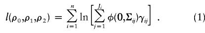For the conditional correlation coefficient of the trait values between members of a sib pair, ρ_i, i=0,1,2, the following order restriction is generally true (Wright 1997): 0<ρ₀⩽ρ₁⩽ρ₂⩽1. When there is no linkage, the correlation coefficient does not depend on the marker allele–sharing status—that is, 0<ρ₀=ρ₁=ρ₂⩽1.

In the present study, we put the following restriction on ρ₀, ρ₁, and ρ₂:

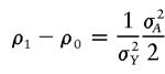
where δ=ρ₂-ρ₀ and f is a prespecified known value. That is, ρ₁ is a convex combination of ρ₀ and ρ₂. The situation without such an assumption will be considered in a separate article. For a model without gene-environment interaction, we have (from Kempthorne [1957] and Tang and Siegmund [2001]):

and

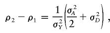where σ²_A and σ²_D are the variances of the additive and dominance effects of the trait, respectively, and σ²_Y is the variance of the trait. It can be seen that f=0.5 (which is equivalent to σ_D=0) represents an additive effect of the trait gene. It can also be seen that ρ₂-ρ₁⩾ρ₁-ρ₀, since σ_D⩾0, suggesting f<0.5 if the dominance variance is present.

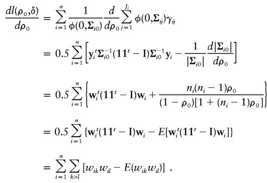
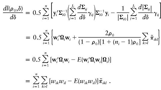
When there is no linkage, δ=0; otherwise, δ>0. Under this parameterization, the unknown parameters in the log-likelihood function in equation (1) becomes (ρ₀,δ) instead of (ρ₀,ρ₁,ρ₂). The log-likelihood function in equation (1) now becomes

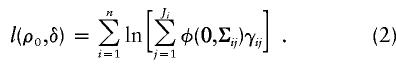The hypotheses of interest are

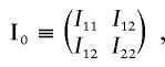
Define . is a measure of the average IBD-sharing extent between the kth sib and the lth sib. When f=0.5, it is the proportion of alleles shared IBD by the kth sib and the lth sib (Haseman and Elston 1972). The distribution of is the same for each pair in each family, regardless of the sibship size. Under the null hypothesis, is independent of y_i. We denote the mean and variance of by and , respectively.

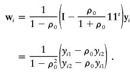
Under the null hypothesis H₀, δ=0 and ρ₀=ρ₁=ρ₂. The matrices Σ_ij, j=1,2,…,J_i, are all the same, with all off-diagonal elements equal to ρ₀. Let this matrix be denoted by Σ_i0. For simplicity, we introduce a vector, w_i=(w_i1,…,w_ini)^t≡Σ^-1_i0y_i. Under the null hypothesis, w_i∼N(0,Σ^-1_i0), since y_i∼N(0,Σ_i0). We note that

where r_i=ρ₀/[1+(n_i-1)ρ₀] and , where is the average of all the elements of y_i.

In what follows, we present a score statistic for testing the hypotheses in equation (3). The first-order derivatives and the information matrix that are necessary for this purpose are presented in Appendix A.

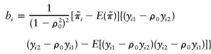
To better describe the score statistic, we define

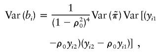
That is, b_i is the inner product of the vector and the vector {w_ikw_il-E(w_ikw_il)}, two vectors each of length 0.5n_i(n_i-1). Under the null hypothesis, the mean and variance of b_i are, respectively, E(b_i)=0 and , since values are independent of w_i when there is no linkage.

It is shown in Appendix B that, to test the null hypothesis H₀ against the alternative hypothesis H_a in equation (3), one can use the following score statistic:

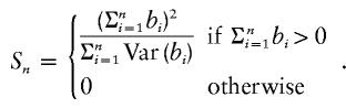In Appendix B, it is derived that S_n is asymptotically distributed as 0.5χ²₀+0.5χ²₁ under the null hypothesis in equation (3).

We note that the mean and variance of are the same for any sib pair in any family. It can be derived from the study by Amos et al. (1989) that and

where p_i is the frequency of the ith marker allele. However, the mean and variance of w_ikw_il depend on the sibship size n_i through r_i:

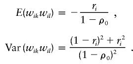These expressions for , and Var(w_ikw_il) can be used in the calculation of the score statistic S_n; however, we do not endorse such a practice. Instead, we recommend using the sample counterparts of these quantities in the calculation of S_n. The main reason is that doing this tends to make the score statistic S_n more robust in situations in which the normality assumption for the trait values is violated and/or the marker locus is in linkage disequilibrium with the trait locus. In the latter case, it is inappropriate to use the population marker-allele frequencies to calculate .

To be specific, we recommend replacing and with the sample mean and the sample variance of {π_ikl} for all sib pairs from all families, respectively, and replacing E(w_ikw_il) and Var(w_ikw_il) with the sample mean and the sample variance of {w_ikw_il} for all sib pairs from all the families that are of the same size, respectively. This is how the score statistic S_n is calculated in our simulation.

When transforming y_i into w_i, we need to know the correlation coefficient, ρ₀, between the trait values of sib pairs. Since the true value of ρ₀ is unknown, we suggest replacing it with the sample correlation coefficient between independent sib pairs. By standard asymptotic theory, since this sample correlation is a consistent estimator of ρ₀, such substitution does not change the asymptotic distribution of S_n.

Data Standardization

In deriving the score statistic S_n, we have assumed that the trait values for a sibship, y_i, have a multivariate normal distribution, conditional on the IBD-sharing configuration within the sibship. The conditional marginal mean and variance for each component of y_i—say, y_ik—are 0 and 1, respectively. This implies that the unconditional marginal mean and variance of y_ik are also 0 and 1, respectively.

When the mean of y_ik is not 0 and the variance of y_ik is not 1, we can standardize y_i in the following way: Consider the trait values of all sibs in all families, {y_ik, k=1,…,n_i, i=1,…,n}. Let and be the sample mean and sample standard deviation, respectively, of these trait values. We standardize y_ik by

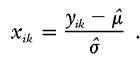Since and are consistent estimators of their respective population counterparts, x_ik has a mean of 0 and a variance of 1, asymptotically. Consequently, the score statistic S_n based on {x_ik} still has the limiting distribution 0.5χ²₀+0.5χ²₁, on the basis of the standard asymptotic theory.

So far, we have critically assumed that y_i has a multivariate normal distribution conditional on the IBD-sharing configuration in the sibship. When this normality assumption is not satisfied, the proposed score statistic S_n may have poor performance. This is also a concern for the H-E method (Allison et al. 1999).

To reduce the impact of nonnormality on the performance of the proposed score statistic, we recommend transforming the trait values first, on the basis of the empirical normal quantile–distribution transformation. The description of this transformation is as follows: Consider the trait values of all sibs in all families, {y_ik,k=1,…,n_i,i=1,…,n}. Let r_ik be the rank of the y_ik. The transformation of y_ik is

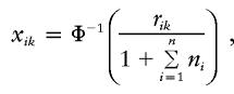where Φ⁻¹ is the inverse of the cumulative function of the standard normal distribution. x_ik is basically the empirical normal quantile distribution transformation of y_ik, since is basically the empirical distribution of all the trait values. We use instead of here, because we want to make sure that x_ik<∞. From standard asymptotic theory, x_ik follows the standard normal distribution, with a mean of 0 and a variance of 1.

We then assume that the joint distribution of x_i=(x_i1,x_i2,…,x_ini)^t is a multivariate normal distribution conditional on the IBD-sharing configuration: for the kth sib and the lth sib, the correlation coefficients between x_ik and x_il are ρ₀, ρ₁, or ρ₂ if they share 0, 1, or 2 alleles IBD, respectively, at the marker locus. This modeling procedure is often referred to as the “multivariate (empirical) normal copula” model. For more discussions about bivariate copula models, see (for example) reports by Genest and MacKay (1986) and Klaassen and Wellner (1997).

It can be shown that such transformation does not change the asymptotic distribution of the likelihood-ratio statistic for the log-likelihood in equation (2) (authors' unpublished data). Since the asymptotic distribution of the score statistic S_n is the same as that of the likelihood-ratio statistic, it follows that such transformation will not change the asymptotic distribution of S_n either.

Special Cases

In the previous section, we derived a score statistic for sibships of arbitrary size. This statistic is related to some other statistics in the literature and has a simple interpretation when the sibship size is constant across all families.

Independent Sib Pairs

For sib-pair data in which n_i=2, i=1,2,…,n, we have

Furthermore,

and

where .

Since

it can be seen that, when f=0.5, is proportional to the estimated slope in the “new combined HE regression” (HE-COM; Sham and Purcell ²⁰⁰¹). In this regression, the dependent variable is

which is a weighted sum of the squared sums and the squared differences, and the independent variable is . Therefore, for independent sib-pair data, the proposed score statistic S_n is equivalent to the t test for testing the regression effect in such a regression. The rejection region of such a test is one sided. Sham and Purcell (2001) compared the performance of the H-E method with some other common statistics; HE-COM outperforms the other statistics in all of the situations investigated.

Constant Sibship Size >2

When the sibship size is constant across all families, the proposed statistic S_n takes a simpler form and is related to the usual F-test statistic for testing whether the regression coefficient is 0 in a regression analysis.

Let s be the common sibship size. We have

where N=0.5ns(s-1) is the total number of sib pairs in all n families. Now E(w_ikw_il) and Var(w_ikw_il) are the same across all families. The nonzero part of S_n becomes

On the other hand, if we regress {w_ikw_il} against {π_ikl}, the usual F statistic for testing whether the regression slope is 0 is equivalent to the quantity on the right hand side in equation (4).

Simulations

In the simulations, we assume that there are three sibs in each family. The trait is assumed to be determined by two equally frequent alleles, D and d, and the marker-allele frequencies are also assumed to be equal. The trait values, (y₁,y₂,y₃), of the three sibs in a family are simulated on the basis of the following model:

where u represents the effect of shared genes other than the one at the locus under consideration or common environmental factors; ε₁, ε₂, and ε₃ are error terms that are independent of each other; and g₁, g₂, and g₃ are the genetic contributions of the linked trait locus, with

The value of μ_dd, μ_Dd, and μ_DD are determined from the broad-sense heritability, h, which, following Gillespie (1998), is defined as

In the above expression, σ²_g, σ²_u, and σ²_ε are the variances due to the quantitative-trait locus, shared gene or environmental effect u, and error ε, respectively.

Specifically, we consider the following four trait models in the simulation:

• Model 1:

  , μ_Dd=0, and μ_DD= -μ_dd. ε_i1 and ε_i2 are independently distributed as N(0,1).

• Model 2:

  , μ_Dd=0, and μ_DD= -μ_dd. ε_i1 and ε_i2 are independently distributed as .

• Model 3:

  , μ_Dd=0.5μ_dd, and μ_DD=-μ_dd. ε_i1 and ε_i2 are independently distributed as N(0,1).

• Model 4:

  , μ_Dd=0.5μ_dd, and μ_DD=-μ_dd. ε_i1 and ε_i2 are independently distributed as .

In all four models, u_i is generated from N(0,0.5).

Models 1 and 2 assume that the mean phenotypes are determined additively by the alleles at the disease locus. Models 3 and 4 introduce some dominance. We note that the error distributions in models 1 and 3 are symmetrical, whereas the error distributions in models 2 and 4 are skewed to the right. Under these four models, the type I error and power of the proposed score statistic and the original H-E statistic (Haseman and Elston 1972) are compared. When calculating the score statistic, we use two methods to standardize the trait values. First, we use the sample mean and sample standard deviation in the way described in the Data Standardization section. The corresponding score statistic is denoted by S^*_n. We also standardize the trait values with the empirical normal quantile distribution transformation, which is also described in that section; the corresponding score statistic is denoted by S^**_n. In calculating the H-E statistic, we treat the three dependent sib pairs formed from the three sibs in the same family as independent sib pairs. Such practice is valid when number of sib pairs is large, as in the situation of our simulation (Blackwelder and Elston 1985; Wilson and Elston ¹⁹⁹³). In all of these analyses, we use an additive model, by setting f=0.5.

The IBD-sharing probabilities at the marker locus are calculated from table II of Haseman and Elston (1972), since it is faster and more convenient than using some existing genetics programs. The simulation program was written in R language (Ihaka and Gentleman 1996). It was run in R (version 1.3.0) on a Compaq XP 1000 workstation running Red Hat Linux 7.1.

In the simulation study of the type I error rate, we set the recombination fraction (θ) between the quantitative-trait locus and the marker at θ=0.5 and set the heritability at h=0. Table 1 reports the observed type I error rates of these three statistics when the nominal significance level is at .1, .05, .01, and .001 and when the number of family members is 100 and 200. For these three statistics, the observed type I error rates are very close to the respective nominal significance levels.

Table 1.

Type I Error Rates Based on 10,000 Replications

	Nominal Significance Level
Model, SampleSize, andScore Statistic	.1	.05	.01	.001
1:
100:
H-E	.0993	.0523	.0120	.0013
S*n	.0996	.0491	.0106	.0014
S**n	.1020	.0484	.0106	.0011
200:
H-E	.1004	.0521	.0113	.0011
S*n	.0999	.0512	.0124	.0018
S**n	.0992	.0514	.0133	.0018
2:
100:
H-E	.1026	.0520	.0109	.0014
S*n	.1043	.0551	.0122	.0013
S**n	.1055	.0547	.0122	.0009
200:
H-E	.1025	.0510	.0115	.0010
S*n	.1047	.0531	.0132	.0018
S**n	.1061	.0550	.0115	.0013
3:
100:
H-E	.1063	.0526	.0112	.0010
S*n	.1023	.0514	.0112	.0012
S**n	.1002	.0519	.0109	.0012
200:
H-E	.0988	.0500	.0095	.0013
S*n	.1015	.0524	.0112	.0018
S**n	.1013	.0531	.0109	.0018
4:
100:
H-E	.1049	.0534	.0110	.0011
S*n	.1049	.0566	.0142	.0014
S**n	.1065	.0555	.0127	.0018
200:
H-E	.1003	.0505	.0114	.0011
S*n	.1011	.0531	.0126	.0012
S**n	.0972	.0497	.0114	.0020

To study the power of the four statistics, we fix θ between the trait locus and the marker at 0. Figures 1 and 2 depict the power of the four statistics when the (broad-sense) heritability h is allowed to change from 0.05 to 0.5 with step size 0.05 for sample sizes 100 and 200. In the four models considered, the score statistics (S^*_n and S^**_n) perform no worse than does the H-E statistic. The difference in their performance is negligible when the heritability is small (h<0.2 for n=100 and h<0.1 for n=200 in models 1 and 3; h<0.1 for n=100 in models 2 and 4). However, for other heritability values, both score statistics perform better than the H-E statistic. The increase in the performance of the two score statistics is more apparent in models 2 and 4, where the error terms are skewed.

Figure 1.

Power at different levels of heritability at the nominal significance level of .001, for 1,000 replicates, with 100 families included in each.

Figure 2.

Power at different levels of heritability at the nominal significance level of .001, for 1,000 replicates, with 200 families included in each.

We compare the two data-standardization techniques, by comparing the performance of S^*_n and S^**_n. For the models where the error terms are normally distributed (i.e., models 1 and 3), the powers of these two score statistics are very close to each other (the powers of these statistics in model 1 are virtually the same). However, for models in which the error terms are skewed (i.e., models 2 and 4), the power of S^*_n is less than the power when the error terms are normally distributed (compare model 3 vs. model 1, and model 4 vs. model 2). However, the power of S^**_n almost remains the same (again, compare model 3 vs. model 1, and model 4 vs. model 2). The empirical normal quantile distribution transformation seems to be more robust to nonnormality of the error terms.

Discussion

In the present study, we proposed a score statistic for detecting linkage to quantitative-trait loci. This score statistic inherits the benefit of the likelihood-ratio statistic, in that it makes efficient use of the information from all sibs in sibships of arbitrary size, yet it is much easier to compute. The ease of computation results from two facts: First, as an intrinsic property, the score statistic does not involve maximization of the likelihood function. Because of the explicit formula for the score statistic, its calculation is straightforward. Second, although the calculation of the likelihood function requires the joint probabilities of the IBD-sharing statuses among all sibs in a sibship, it turns out that it suffices to know the pairwise IBD-sharing probabilities in order to calculate the score statistic. Since several genetics programs exist that can export pairwise IBD-sharing probabilities between sib pairs, the calculation of the proposed score statistic can be implemented very easily. This second advantage of the score statistic over the likelihood-ratio statistic is important here, because it makes the calculation of the score statistic immediately feasible in that it does not require the joint sharing probabilities among all sibs in a sibship. Tang and Siegmund (2001) considered a score statistic in a similar context, but it was assumed that the markers were completely informative, in which case the IBD-sharing configuration among a sibship would be known with certainty.

In comparison with the H-E method and its recent modifications, a salient feature of the proposed score statistic is that it handles multiplex sibships in a natural way. Without breaking the sibship into sib pairs, the proposed score statistic is calculated directly from the sibship. For independent sib pairs, this score statistic turns out to be asymptotically equivalent to the HE-COM statistic of Sham and Purcell (2001).

In our simulation study, we considered one additive model and one dominant model. For each model, we considered the cases where the error terms are symmetrical (normally distributed) and skewed (χ² distributed). Under these simulation models, the proposed score statistic outperforms the H-E method, in terms of power, when the heritability changes from 0.05 to 0.5. The type I error rates of the score statistic and the H-E method are both well under control.

For nonnormal data, we recommend a data-transformation procedure that is based on the standard normal density function and the empirical distribution of the trait values. As pointed out by an anonymous reviewer, such a data-transformation procedure can be done prior to any other quantitative-trait loci mapping method, and this does not guarantee multivariate normality. The latter point is the reason that we used the normal copula model; we assume that the transformed data have a multivariate normal distribution. As the same reviewer pointed out, such a practice could complicate the interpretation of some interesting quantities such as additive variance and heritability; however, as far as the test is concerned, we have shown that, for the model used in our study, such a transformation does not change the asymptotic distribution of the score statistic we derived (authors' unpublished data).

Compared with our likelihood function (2), the variance-component analysis uses a different but related likelihood function. In likelihood function (2), the likelihood for the ith family is a mixture of J_i normal densities. A corresponding variance-component likelihood function would be

where Σ_i is a symmetric matrix whose diagonal elements are 1 and whose klth off-diagonal element is

We prefer likelihood function (2) to likelihood function (5), because the former contains more information; one can write out likelihood function (5) from likelihood function (2), but not vice versa. If the normality assumption holds, the analysis based on the former should have as much power as that based on the latter. In a simulation study, the likelihood-ratio statistic from likelihood function (2) performs better than that from likelihood function (5) (Dolan et al. 1999). We expect our score statistic to be more robust against violation of the normality assumption, in terms of type I error rate; the asymptotic distribution of a score statistic relies solely on the central limit theorem, although the derivation of the score statistic depends on the model assumption. In contrast, the asymptotic distribution of the likelihood-ratio statistic is directly related to the model assumption. Further studies are needed to assess the power behavior of our approach and of the variance-component method for non-normal data.

We note that likelihood function (2) is based on the joint distribution of marker and trait. Thus, this likelihood is only correct for randomly selected families and is approximately correct for moderately selected sibship data. This likelihood cannot be simply applied to extremely discordant sib-pair data. However, analysis of extremely discordant sib-pair data can be considered to be a missing-data problem—that is, the pairs not selected for genotyping can be viewed as having their marker data missing. For instance, one approach for applying our method to extremely discordant sib-pair data is to include all the untyped pairs and assign the prior IBD-sharing probabilities to these pairs (Kruglyak and Lander 1995; Eaves et al. ¹⁹⁹⁶; Dolan et al. ¹⁹⁹⁹). Other approaches for analyzing extremely discordant sib-pair data include the method based on IBD-sharing scores or weighted IBD-sharing scores (Risch and Zhang 1995; Gu et al. ¹⁹⁹⁶) or the method based on the conditional likelihood of marker data, given trait values (Dudoit and Speed 1999; Sham et al. ²⁰⁰⁰; Goldstein et al. ²⁰⁰¹).

In the present study, we considered only the sib-sib relationship; however, the score statistic can also be applied directly in situations where there is only one relationship involved, no matter what that relationship is. When there is more than one relationship, the situation becomes more complicated. The score statistic that can handle multiple relationships together will be presented in a separate article.

Appendix A: Derivatives and Information Matrix

Let Ω_i be a symmetrical matrix whose diagonal elements are all 0 and whose klth off-diagonal element is . It is apparent that .

When evaluated at (ρ₀,δ)=(ρ₀,0), the derivative of l(ρ₀,δ) with respect to ρ₀ is

Similarly, the derivative of l(ρ₀,δ) with respect to δ, when evaluated at (ρ₀,δ)=(ρ₀,0), is

In deriving these first-order derivatives, we used the following facts:

• 1.  dΣ-1i0/dρ0=-Σ^-1_i0 dΣi0/dρ0Σ^-1_i0=-Σ^-1_i0(11^t-I)Σ^-1_i0,
• 2. ,
• 3. |Σ_i0|=(1-ρ₀)^n_i-1[1+(n_i-1)ρ₀],
• 4. . (The proof of this fact is omitted, because of its length.)

The expectations of w^t_i(11^t-I)w_i and the conditional expectation of w^t_iΩ_iw_i are taken under the null hypothesis, and are

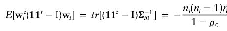and

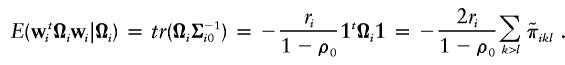The information matrix is

where

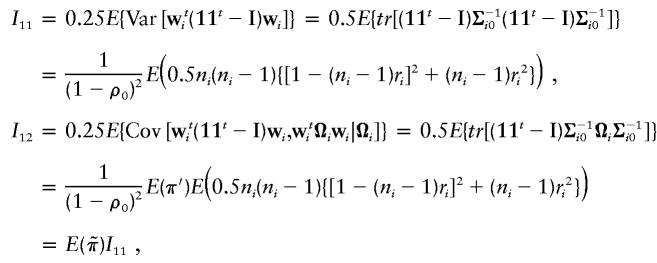and

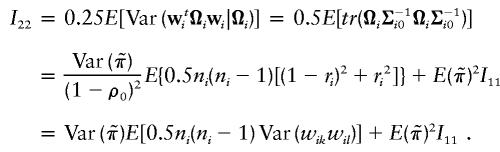In the final expressions for I₁₁, I₁₂, and I₂₂, the expectation is taken with respect to the sibship size n_i.

Appendix B : Derivation of the Score Statistic S_n

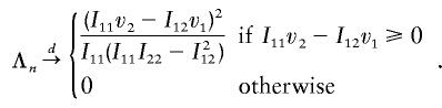
From asymptotic theory, under the null hypothesis,

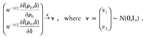Let Θ₀={(ρ₀,δ):δ=0} and Θ₁={(ρ₀,δ):δ>0} be the sets of parameters that correspond to the null hypothesis and the alternative hypothesis, respectively. Let 𝔥₀={h=(h₁,h₂):h₁∈R,h₂=0} and 𝔥₁={h=(h₁,h₂):h₁∈R,h₂>0}. From theorem 16.7 of van der Vaart (1998), the likelihood ratio statistic is

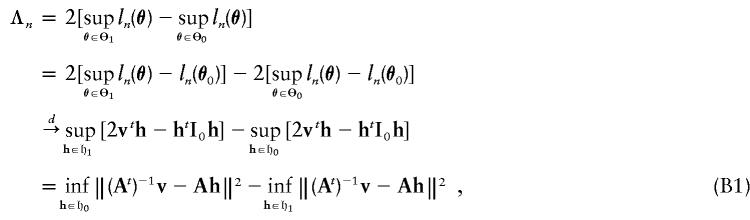where

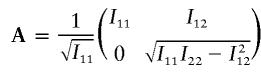Notice that A^tA=I₀ and (A^t)^-1v∼N(0,I), where I is a 2×2 identity matrix.

The parameter space 𝔥₁ is the upper-half space. Since Ah∈𝔥₀ if and only if h∈𝔥₀, and since Ah∈𝔥₁ if and only if h∈𝔥₁, {Ah:h∈𝔥₁} is also the upper-half space. Since

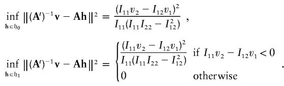Therefore, from equation (B1),

whose distribution is 0.5χ²₀+0.5χ²₁.

Since

a consistent estimator of I₁₁I₂₂-I²₁₂ is

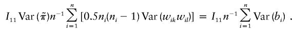A sample version of I₁₁v₂-I₁₂v₁ is

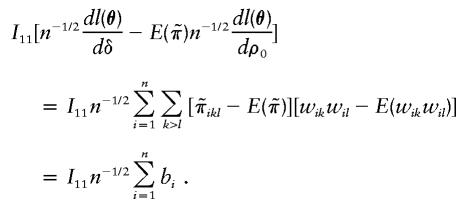Therefore, a sample version of (I₁₁v₂-I₁₂v₁)²/[I₁₁(I₁₁I₂₂-I²₁₂)] is (Σⁿ_i=1b_i)²/Σⁿ_i=1Var(b_i), which is the score statistic S_n reported in the text.

References

- Allison DB, Neale MC, Zannolli R, Schork NJ, Amos CI, Blangero J (1999) Testing the robustness of the likelihood-ratio test in a variance-component quantitative-trait loci–mapping procedure. Am J Hum Genet 65:531–544 [DOI] [PMC free article] [PubMed] [Google Scholar]
- Almasy L, Blangero J (1998) Multipoint quantitative-trait linkage analysis in general pedigrees. Am J Hum Genet 62:1198–1211 [DOI] [PMC free article] [PubMed] [Google Scholar]
- Amos CI, Elston RC, Wilson AF, Bailey-Wilson JE (1989) A more powerful robust sib-pair test of linkage for quantitative traits. Genet Epidemiol 6:435–449 [DOI] [PubMed] [Google Scholar]
- Blackwelder WC, Elston RC (1985) A comparison of sib-pair linkage tests for disease susceptibility loci. Genet Epidemiol 2:85–97 [DOI] [PubMed] [Google Scholar]
- Collins A, Morton NE (1995) Nonparametric tests for linkage with dependent sib pairs. Hum Hered 45:311–318 [DOI] [PubMed] [Google Scholar]
- Dolan CV, Boomsma DI, Neale MC (1999) A simulation study of the effects of assignment or prior identity-by-descent probabilities to unselected sib pairs, in covariance-structure modeling of a quantitative-trait locus. Am J Hum Genet 64:268–280 [DOI] [PMC free article] [PubMed] [Google Scholar]
- Dudoit S, Speed TP (1999) A score test for linkage using identity by descent data from sibships. Ann Stat 27:943–986 [Google Scholar]
- Eaves LJ, Neale MC, Maes H (1996) Multivariate multipoint linkage analysis of quantitative trait loci. Behav Genet 26:519–525 [DOI] [PubMed] [Google Scholar]
- Elston RC, Buxbaum S, Jacobs KB, Olson JM (2000) Haseman and Elston revisited. Genet Epidemiol 19:1–17 [DOI] [PubMed] [Google Scholar]
- Forrest WF (2001) Weighting improves the ‘new Haseman-Elston’ method. Hum Hered 52:47–54 [DOI] [PubMed] [Google Scholar]
- Fulker DW, Cherny SS (1996) An improved multipoint sib-pair analysis of quantitative traits. Behav Genet 26:527–532 [DOI] [PubMed] [Google Scholar]
- Fulker DW, Cherny SS, Cardon LR (1995) Multipoint interval mapping of quantitative trait loci, using sib pairs. Am J Hum Genet 56:1224–1233 [PMC free article] [PubMed] [Google Scholar]
- Genest C, MacKay J (1986) The joy of copulas: bivariate distributions with uniform marginals. Am Statistician 40:280–283 [Google Scholar]
- Gillespie JH (1998) Population genetics: a concise guide. Johns Hopkins University Press, Baltimore [Google Scholar]
- Goldstein DR, Dudoit S, Speed TP (2001) Power and robustness of a score test for linkage analysis of quantitative traits using identity by descent data on sib pairs. Genet Epidemiol 20:415–431 [DOI] [PubMed] [Google Scholar]
- Gu C, Todorov A, Rao DC (1996) Combining extremely concordant sib pairs with extremely discordant sib pairs provide a cost effective way to linkage analysis of quantitative trait loci. Genet Epidemiol 13:513–533 [DOI] [PubMed] [Google Scholar]
- Haseman JK, Elston RC (1972) The investigation of linkage between a quantitative trait and a marker locus. Behav Genet 2:3–19 [DOI] [PubMed] [Google Scholar]
- Ihaka R, Gentleman R (1996) R: a language for data analysis and graphics. J Comp Graph Stat 5:299–314 [Google Scholar]
- Kempthorne O (1957) An introduction to genetic statistics. Wiley, New York [Google Scholar]
- Klaassen CAJ, Wellner JA (1997) Efficient estimation in the bivariate normal copula model: normal margins are least favorable. Bernoulli 3:55–77 [Google Scholar]
- Kruglyak L, Lander ES (1995) Complete multipoint sib-pair analysis of qualitative and quantitative traits. Am J Hum Genet 57:439–454 [PMC free article] [PubMed] [Google Scholar]
- Risch N, Zhang H (1995) Extreme discordant sib pairs for mapping quantitative trait loci in humans. Science 268:1584–1589 [DOI] [PubMed] [Google Scholar]
- Sham PC, Purcell S (2001) Equivalence between Haseman-Elston and variance-components linkage analyses for sib pairs. Am J Hum Genet 68:1527–1532 [DOI] [PMC free article] [PubMed] [Google Scholar]
- Sham PC, Zhao JH, Cherny SS, Hewitt JK (2000) Variance-components QTL linkage analysis of selected and non-normal samples: conditioning on trait values. Genet Epidemiol 10 Suppl 1:S22–S28 [DOI] [PubMed] [Google Scholar]
- Tang HK, Siegmund D (2001) Mapping quantitative trait loci in oligogenic models. Biostatistics 2:147–162 [DOI] [PubMed] [Google Scholar]
- Tiwari HK, Elston RC (1997) Linkage of multilocus components of variance to polymorphic markers. Ann Hum Genet 61:253–261 [DOI] [PubMed] [Google Scholar]
- van der Vaart AW (1998) Asymptotic statistics. Cambridge University Press, New York [Google Scholar]
- Wang D, Lin S, Cheng R, Gao X, Wright FA (2001) Transformation of sib-pair values for the Haseman-Elston method. Am J Hum Genet 68:1238–1249 [DOI] [PMC free article] [PubMed] [Google Scholar]
- Wilson AF, Elston RC (1993) Statistical validity of the Haseman-Elston sib-pair test in small samples. Genet Epidemiol 10:593–598 [DOI] [PubMed] [Google Scholar]
- Wright FA (1997) The phenotypic difference discards sib-pair QTL linkage information. Am J Hum Genet 60:740–742 [PMC free article] [PubMed] [Google Scholar]
- Xu X, Weiss S, Xu XP, Wei LJ (2000) A unified Haseman-Elston method for testing linkage with quantitative traits. Am J Hum Genet 67:1025–1028 [DOI] [PMC free article] [PubMed] [Google Scholar]