The four ingredients of single-sequence RNA secondary structure prediction. A unifying perspective

Abstract

Any method for RNA secondary structure prediction is determined by four ingredients. The architecture is the choice of features implemented by the model (such as stacked basepairs, loop length distributions, etc.). The architecture determines the number of parameters in the model. The scoring scheme is the nature of those parameters (whether thermodynamic, probabilistic, or weights). The parameterization stands for the specific values assigned to the parameters. These three ingredients are referred to as “the model.” The fourth ingredient is the folding algorithms used to predict plausible secondary structures given the model and the sequence of a structural RNA. Here, I make several unifying observations drawn from looking at more than 40 years of methods for RNA secondary structure prediction in the light of this classification. As a final observation, there seems to be a performance ceiling that affects all methods with complex architectures, a ceiling that impacts all scoring schemes with remarkable similarity. This suggests that modeling RNA secondary structure by using intrinsic sequence-based plausible “foldability” will require the incorporation of other forms of information in order to constrain the folding space and to improve prediction accuracy. This could give an advantage to probabilistic scoring systems since a probabilistic framework is a natural platform to incorporate different sources of information into one single inference problem.

Introduction

Methods for RNA secondary structure prediction based on thermodynamic parameters were already introduced in the 1980s.^1-4 These still widely used thermodynamic methods owe their success to the incorporation of a large number of folding features (in addition to the standard basepairs), and to a carefully crafted experimental estimation of those thermodynamic parameters.^5-12 The collection of thermodynamic parameters is usually referred to as the nearest-neighbor model of RNA folding because it puts special emphasis on the thermodynamics of basepair correlations with their most adjacent bases (whether paired or unpaired). Indeed, their success has been such that more than 40 years later, the most widely used methods for RNA secondary structure prediction are thermodynamic, and not very different from the original ones. Representative examples are: Mfold/UNAFold,^13,14 ViennaRNA^15,16 and RNAstructure.^10,17 Despite their durability, it has become apparent that the folding accuracy of the thermodynamic methods is relatively poor.^11,18-20

By the 1990s, probabilistic models were brought into the problem of RNA structure prediction.^21-24 Prior to these approaches, probabilistic models had been introduced for the related problem of RNA homology detection using a consensus secondary structure, for which a “profile model” is built with position-specific scores.^25,26 All these early probabilistic methods used RNA secondary structure in combination with other sources of information (whether comparative analysis, covariation, alignments or others). For instance, the method Pfold^22,27 informs the likelihood of two positions being basepaired by looking at the pattern of covariation of those two positions in an input alignment. QRNA, in addition to using an input (pairwise) alignment to inform the likelihood of any two positions being basepaired, also uses the alignment to analyze the multiple-of-three patterns of mutations in order to infer the likelihood of the sequence being protein coding.²⁴ The profiled probabilistic models for RNA homology use RNA structural covariation in combination with sequence conservation to improve homology detection.²⁸ Other probabilistic methods implemented afterward also integrate different forms of information.²⁹

One limitation of thermodynamic models is that their parameterization (i.e. selection of parameter values) is laborious, since it requires calorimetry measurements of many model RNA structures. For instance, there are very good estimations of stacking free-energies for basepairs (that is, the free-energy of a basepair as it stacks onto another contiguous pair), but other parameters such as those for multi-loop features have to be guessed due to lack of thermodynamic information.

The labor-intensive nature of obtaining thermodynamic parameters is a motivation for exploring alternative approaches that can be trained statistically using structural data. We use the term “statistical” to describe all methods that train their parameters using known RNA structures. Statistical methods can, in turn, be separated into probabilistic and “weights” methods depending on the nature of their parameters. Among statistical methods, probabilistic models have the additional advantage of being easy to train for arbitrary types of features. A seminal work in 2004 used this advantage in order to explore a collection of about 10 simple different model architectures using probabilistic scores.³⁰ Results showed that some models with about 20 parameters perform surprisingly close to the standard thermodynamic models using thousands of parameters.

Alternatively, statistical non-probabilistic “weights” methods have been introduced in recent years. Examples are CONTRAfold,^31,32 Simfold^33,34 and ContextFold.³⁵ These statistical methods use complex architectures similar to those of the thermodynamic models, and they seem to outperform thermodynamic methods.³⁶

As late as 2009, all published probabilistic methods for RNA secondary structure had been models with no more than 100 parameters, while the contemporary statistical non-probabilistic models included complexities similar to those of the thermodynamic models. This historical accident introduced an otherwise unfounded belief that complex models of RNA secondary structure could not be paired with probabilistic scoring schemes.³¹ Since then, several efforts toward more complex probabilistic models of RNA secondary structure have been presented.^37,38 Recently, explicit implementations of probabilistic models expressing the same complex features as the thermodynamic models and more, while using a comparable number of parameters, has been presented.³⁹

Probabilistic models, in addition to being comparable to other methods in the complexity of features they can incorporate, are useful for exploring the relative importance of different features of RNA secondary structure going beyond the complexities of the thermodynamic models. TORNADO, a compiler that can parse a wide range of RNA architecture, has explored into this space.³⁹ The results were somewhat disappointing. Improvements can be found, but RNA folding accuracies using probabilistic models are just slightly above those of other statistical methods such as CONTRAfold. In addition, statistical methods with large number of parameters are easy to overtrain, and the usual data sets that people use to train/test these methods^33,34,40 are quite vulnerable because of a lack of sufficient structural diversity within the data set.

The literature, and even this brief historical review of it, may give the impression that those different methods (thermodynamic, statistical probabilistic or statistical using unconstrained weights) have little in common with each other. In this manuscript, I would like to show that they share fundamental principles, and that looking at what makes the methods similar (as opposed to different) helps us understand the overall problem, and suggests ways of moving forward.

The Four Elements of an RNA Secondary Structure Prediction Algorithm

The four elements necessary (and sufficient) to specify a single-sequence RNA secondary structure prediction method are: the architecture (or number of parameters), the scoring scheme (or nature of the parameters: thermodynamic, probabilistic or weights), the parameterization (or actual values of the parameters) and the folding algorithms. A brief summary of these elements is described in Figure 1. Next, I explore in some depth each of these four components, which will lead to some unifying observations.

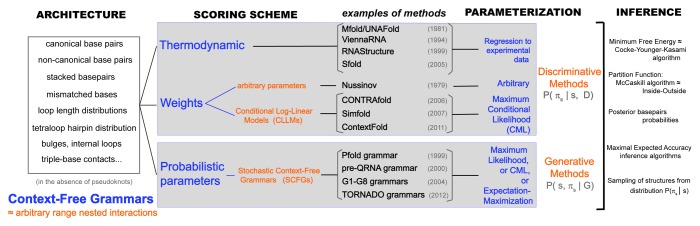
Figure 1.Unified description of different methods for single-sequence RNA secondary structure prediction. The menu of elements that define a method are: architecture, scoring scheme, parameterization and inference method. The architecture consists of the list of features which, in turn, determine the number of parameters of the model. The different architectures one can devise for a nested RNA secondary structure all fall into the category of a Context-Free Grammar (CFG). Any architecture can be implemented using either thermodynamic, weights or probabilistic parameters. Both weight and probabilistic schemes can be trained on data (statistical). There are statistical weight schemes such as CLLMs. Statistical probabilistic schemes for RNA folding are usually stochastic CFGs (SCFGs). Notice that SCFGs are a subset of CFGs. SCFGs describe models with a probabilistic scheme, while the concept CFG applies to all scoring schemes. The assignment of values for the parameters (parameterization) depends on the scoring scheme used. Thermodynamic models take values as kcal/mol free-energy estimations from experimental data. Conditional Log-Linear models use methods that require numerical optimization (CML and also online training). Probabilistic models are usually trained by maximum likelihood methods, which simply require obtaining frequencies of occurrences in the training set [and the addition of at least Laplace (+1) priors]. Once an architecture, scoring scheme and parameterization are in place (that is, a “model”), one can use different algorithms to infer plausible secondary structures. Unlike training, which is specific for the different scoring schemes, the folding algorithms (usually dynamic programming algorithms) are essentially identical for all parameterizations (although oftentimes they have different names). A side note; the term “probabilistic” often leads to confusion. In the end, all scoring schemes (probabilistic or not) can give us insight into the probabilistic distribution of structures (π_s) for a given sequence (s) (the so-called Boltzmann ensemble in a thermodynamic scheme). For instance, one can calculate the distribution’s partition function (via the McCaskill or inside algorithms) or rigorously sample structures from that distribution. However, what is normally referred to as a “probabilistic” model is one in which the parameters of the model are themselves probabilities. Probabilistic models are “generative” models, which means that in addition to the Boltzmann ensemble per sequence, they also provide insight into the joint distribution for the ensemble of sequences and structures. With a probabilistic method, one can quite naturally generate sequences together with their structures according to the model.

Up front, the observations are: (1) Any architecture for RNA secondary structure can be described in the form of a grammar in the Chomsky sense.⁴¹ (2) Although historically it was believed that probabilistic scoring schemes could not be used for architectures with thousands of parameters, it has been shown that architectures of arbitrary complexity can be paired with all three scoring systems. (3) While the parameterization methods are specific for each scoring scheme, the folding algorithms are essentially identical for all scoring types. (4) For all architectures tested, folding algorithms that take into account the whole ensemble of possible structures outperform simpler “best structure” algorithms. This result holds true across all different scoring schemes. (5) For complex architectures, models using either trained probabilities or trained weights predict RNA secondary structures with higher accuracy than methods based solely on thermodynamic parameters. (6) Proper training and testing of methods for RNA secondary structure prediction with large numbers of parameters require using test sets with different structures (not just with different sequences) from the training sets. The current data sets of structural RNAs lack sufficient structural diversity for a proper parameterization and testing of these complex methods.

Architecture

RNA secondary structure is defined by the hydrogen-bond interactions (in cis) between the Watson-Crick faces of two nucleotides located an arbitrary distance apart in the RNA backbone. RNA secondary structure basepairs are usually of the form A-U (U-A), C-G (G-C) and G-U (U-G), although other pairs occur at lower frequency. The Watson-Crick/Watson-Crick basepairs in cis are often referred to as the canonical basepairs. Other hydrogen-bond interactions involving other faces (there are three per nucleotide: Watson-Crick, Sugar or Hoogsteen) or conformations (cis or trans) are oftentimes referred to as the non-canonical basepairs⁴² and, in turn, they determine the tertiary structure of the molecule.

Canonical basepairs usually occur in conjunction with other canonical basepairs forming short helices (or stems) that give stability to the molecule. RNA helices can get interrupted by unpaired nucleotides. Most RNA helices are nested within each other (that is, with no crossing basepairs). Independent helices (or groups of nested helices) tend to aggregate next to each other in crystal structures, oftentimes stacked coaxially forming longer stems. However, a small fraction of basepairs appear in non-nested configurations named pseudoknots. In this review, I concentrate on methods for RNA secondary structure prediction leaving aside pseudoknots as well as tertiary interactions. Although one should not forget that it might be exactly pseudoknots and tertiary interactions what could make the methods move forward and to obtain better prediction accuracies.

An important advance was the realization that any nested (i.e. secondary structure) existing method for RNA folding could be represented as a context-free grammar (CFG),⁴¹ and that RNA secondary structure prediction could be viewed as CFG parsing.⁴³ A CFG consists of non-terminals (NTs) (represented with capital letters), terminals (the actual RNA bases, represented with lower case letters) and production rules of the form [NT - > (any combination of NTs/terminals)]. The production rules determine recursively the strings of RNA bases and structures that the grammar permits.⁴⁴ Grammar for RNA folding allow all possible strings of nucleotides (possibly with some restrictions in the secondary structures allowed), but they “weight” each string differently according to a scoring system that assigns values to the parameters of the grammar. Grammar parameters that provide scores for the actual nucleotides are named “emissions.” Parameters that weight the different choices (rules) for a given non-terminal are named “transitions.” I will discuss the different scoring schemes and how to assign actual values to the parameters in the next sections. Here, I concentrate in the different CFG rules used to describe RNA secondary structure.

A production rule that represents the formation of a basepair is of the form (S - > a S â) where a and â stand for two paired bases. A scoring system for this one-rule grammar requires assigning 16 (or six) parameters whether one allows all possible nucleotides pairs or just restricted (A-U, G-C or G-U) basepairs. This “grammar” would produce a single infinitely long helix of all paired RNA bases. Not quite exactly what we want.

A grammar that produces discontinuous helices with single-stranded bases connecting the stems, and generates independent as well as nested stems could have the form,⁴³

S - > a S â | a S | S a | S S | ε.

This grammar has five rules, here separated by a | (“or” symbol). The fourth rule allows the possibility of multiple helices, and the fifth rule ends a string. The grammar allows one to introduce 16 (or six) basepair emissions, four single base emissions and five transitions one for each of the rules.

The sequence of grammar rules necessary to produce a given RNA structure in named a derivation (or parse). A possible derivation under the above grammar for the toy stem “cacccug” (where nucleotides c-g and a-u are paired to each other) is

S = > c S g = > ca S ug = > cac S ug = > cacc S ug = > caccc S ug = > caccc ε ug.

Double arrows ( = > ) are used for derivations, while single arrows (- > ) are used for depicting the rules of the grammar.

The above grammar serves the purpose of illustrating a simple architecture for RNA secondary structure prediction. However, it has some undesirable properties, mainly “ambiguity,” which means that certain structures can be obtained in many different ways (parses) from the grammar. In an ambiguous grammar, one needs to be careful to consider the contributions of all the possible parses in order to correctly calculate the weight (or probability) of a given structure.⁴⁵ In our toy example, one can easily see that the three unpaired c’s could have been produced by any combination of the (S - > aS) or (S - > Sa) rules, leading (for large RNAs) to a combinatorial explosion of grammar parses representing the same structure. To avoid this potential complication, it is always convenient to work with unambiguous grammars (that is, grammars that guarantee one unique parse per structure).

The Nussinov grammar, one of the first introduced for RNA folding¹ is unambiguous, and has the form

S - > S a | S a S â | ε.

Another grammar also unambiguous with three instead of one non-terminal but similar number of emission parameters is the g6 grammar³⁰ first introduced with the method Pfold²²

S - > L S | L # select left-most helix or base or | final helix or base

L - > a F â | a # helix starts (emit first basepair) or | one single nucleotide emission

F - > a F â | L S # helix continues (emit another basepair) or | hairpin, internal and multifurcation loops

The g6 grammar performs surprisingly better than the Nussinov and other similar grammars, when they all are trained on the same data.³⁰ Later, when we look at different scoring schemes for these two grammars, one can understand what causes this difference in performance.

The standard thermodynamic nearest-neighbor model is more complex and realistic than the grammars presented so far.⁷ Each of the features of RNA secondary structure that the nearest-neighbor model scores can also be represented as a grammar. This is key to understanding how the thermodynamic parameters can be separated from the model architecture; and how parameter values other than thermodynamic free-energies could be used with the same “nearest-neighbor architecture.”

Notice that they may be fewer actual parameters used than parameters originally described by the CFG. Parameters for different grammar rules can be tied together instead of considering them all independent from each other. Selecting the effective number of parameters is a design choice often guided by avoiding an excessive number of free parameters. In Table 1, we report for each architecture the number of “free tied parameters,” that is, independent parameters after tying equivalences have been established.

Table 1. Comparison of different methods for RNA secondary structure prediction.

Method	Architecture # free tied parameters		Scoring scheme	Parameterization	Training datasets	Folding method	Benchmark Set best F (%)
	(6 bps)	(16 bps)					TestSetA	TestSetB
g6	11	21	probabilistic	ML	TrainSetA+2*TranSetB	c-MEA	49.1	47.5
●basic grammar	532	572	probabilistic	ML	TrainSetA+2*TranSetB	c-MEA	56.9	56.5
⋄CONTRAfold v2.02	~300	­-	weights	CML	S-Processed-TRA	c-MEA	57.2	57.9
●CONTRAfoldG	1,278	5,448	probabilistic	ML	TrainSetA+2*TranSetB	c-MEA	58.3	58.6
⋄UNAFold-3.8	~3,500	-	thermodynamic	fit to exp. data	-	CYK	51.0	51.3
⋄Simfold BL*	~as above	-	weights	CML	S-Processed-TRA	CYK	56.5	55.3
⋄RNAstructure v5.2	~12,700	-	thermodynamic	fit to exp. data	-	GCE	53.5	53.8
⋄ViennaRNA v1.8.4	~as above	-	thermodynamic	fit to exp. data	-	GCE	53.7	54.3
●ViennaRNAG	14,307	90,497	probabilistic	ML	TrainSetA+2*TranSetB	c-MEA	60.2	59.4
●ViennaRNAGz_bulge2_ld_mdangle	14,557	91,997	probabilistic	ML	TrainSetA+2*TranSetB	c-MEA	60.5	59.5
⋄ContextFold v1.00	205,000	-	weights	online CML	S-Full	CYK	64.4	49.0

Models. Models with a “⋄” are versioned stand-alone packages. Models with a “^●” are CFGs (with alternative scoring schemes) introduced in reference 39. In particular, ViennaRNAG is a CFG that when parameterized with thermodynamic scores reproduces the ViennaRNA v1.8.4 method, and CONTRAfoldG is another CFG that when parameterized with particular scores reproduces CONTRAfold v2.02. Here, we present the results of probabilistic parameterizations for those grammars. Parameters. Methods are order by increasing number of parameters. Here we report the effective free parameters after tying. (The number of parameters for some of the native thermodynamic methods is only approximate and corresponds to two different versions of the nearest-neighbor model.) Test sets. TestSetA is a well curated collection of sequences from about 10 bona-fide RNA structures. TestSetB includes a collection of about 22 different RNA structure obtained from Rfam v10.0. TestSetA and TestSetB are structurally dissimilar, and they have been defined in reference 39. Performance accuracy. We use F (the harmonic mean of sensitivity and positive predictive value), such that an F of 100% would mean perfect prediction. Performance accuracy is calculated for the entire test set of sequences (instead of averaging the accuracy of each individual sequence). This “total” measures tend to be smaller than those obtained by averaging over sequences because it corrects for the (usually abundant) small sequences in the test sets for which prediction is much easier than for longer sequences. For methods that use a MEA algorithm with a tunable parameter (both c-MEA³¹ and GCE³⁶), this table report the “best F” in the ROC curve between sensitivity and positive predictive value (see ref. 39 for more details). Training sets. Provenance of training sets is as follows: TrainSetA+ 2*TrainSetB ,³⁹ S-Processed-TRA,³³ S-Full.³⁴

Next comes a description of several relevant features of the nearest-neighbor architecture depicted as CFG rules. Theory suggested that RNA stability is more a function of “stacking” of basepairs than H-bond face interaction alone, thus “stacking” is inherent to the nearest-neighbor architecture.^5-7 A rule that would produce stacked pairs is of the form

stacked basepairs (S^cĉ - > a S^aâ â),

in which a basepair (a, â) depends on the contiguous basepair (c, ĉ). This rule is short notation for 16 (or six) rules, and each of them requires 16 (or six) parameters.

Examples of other nearest-neighbor features implemented by the thermodynamic models are,

left and right dangles (P^c,ĉ - > a F | F a),

in which a single left (or right) base depends on the adjacent basepair. Here, P stands for a “paired” non-terminal and F for an arbitrary nonterminal.

Basepairs depending on left and right dangles (P^c - > a F â) (P^c,d - > a F â),

in which a basepair (a, â) depends on the contiguous unpaired bases (c), (d) or both.

Another type of feature fundamental in the nearest-neighbor architecture that extends beyond the simpler grammars above is that of loop length distributions.

Hairpin loops [P - > (m...m)],

a closing rule that places a hairpin loop. This compact representation indicates a finite number of possible loops. There are many different ways to assign parameters to this rule. Below there are two examples,

hairpin loops under independence assumption (P - > a₁a₂a₃|a₁a₂a₄|…|a₁…a_n).

This rule allows hairpin loops with lengths ranging from three to N, and their relative weights are determined by N-2 transition parameters. All bases in a given hairpin loop are emitted independently according to a unique set of four parameters for the nucleotide emission.

Hairpin with exactly four bases (tetraloops) (P - > a₁a₂a₃a₄).

Special rule for tetraloops. This rule uses a set of 4⁴ parameters to describe all possible tetraloops.

Bulge loops (left and right) [P - > (m...m) F] [P - > F (m...m)].

Internal loops [P - > (m...m) F (m...m)],

similar to the above but where the unpaired bases appear on both sides of the basepair.

The nearest-neighbor model does also consider neighboring information for the loops, such as,

tetraloops depending on closing basepair (P^c,ĉ - > a₁a₂a₂a₄).

Hairpin loops with exactly four bases depending on the closing basepair (c, ĉ).

Hairpin mismatches [P^c,ĉ - > a (m...m) b],

in which the final two bases of a hairpin loop (a, b) depend on the closing basepair (c, ĉ).

Dangles in bulges [P^c,ĉ - > a(m...m) b F b],

in which the end base (a) of a bulge depends on the adjacent basepair (c, ĉ), and the closing basepair (b, $\widehat{b}$) depends on the adjacent bulge base.

Internal loop mismatches [P^c,ĉ - > a(d...) b F b (...d)e ],

where for an internal loop limited by the two basepairs (c, ĉ) and (b, b), the closing bases (a, e) depend on the adjacent basepair (c, ĉ), and the basepair (b, b) depends on the adjacent bases in the internal loop.

A complete context-free grammar that implements all the features of the nearest-neighbor model can be found in reference.³⁹ A simpler grammar that includes the basic features of those models but with stacking, dangles and mismatches removed can be an instructive simplification. That simpler grammar, which can be viewed as a “scaffold” for the nearest-neighbor model, has the form

S - > a S | F S | ε # Start: find a left base, or a left Helix or End

F - > a F â | a P â # Helix continues | Helix ends

P - > m...m # Hairpin Loop

P - > m...m F | F m...m # Left or Right Bulge

P - > m...m F m...m # Internal Loop

P - > M1 M # Multiloop two or more Helices

M - > M1 R | R # One or more Helices

M1 - > a M1 | F # One Helix, possibly with single left unpaired bases

R - > R a | M1 l # Last Helix, possibly with left and right unpaired bases.

This basic grammar has six non-terminals. Non-terminal “F” corresponds to a helix. Non-terminal “P” corresponds to all possible types of loops. The possible loop fates are: a hairpin loop, a left or right bulge continued by another helix, an internal loop also continued by another helix or a multi-loop with possibly unpaired bases and including at least two more helices. This distinction between different types of loops is at the core of the nearest-neighbor model, and it is missing in the simpler g6 grammar described before.

All these complex features were first introduced by the nearest-neighbor model and adopted right away by the thermodynamic methods.³ At present, complex features have been explored by all possible scoring schemes. For example, the statistical method CONTRAfold uses an architecture that follows closely the nearest-neighbor model, but they maintain a relatively small number of free (tied) parameters in order to keep the training under control, and in reference 39, CFGs mimicking the architectures of both CONTRAfold and ViennaRNA have been presented.

Statistical methods both probabilistic and using real-valued weights have explored an even larger range of parameters than the nearest-neighbor model. For example, in the method ContextFold, higher than first-order Markov dependencies have been considered such as (see ref. 35 for more details),

one or more unpaired bases depending on several other bases [ P^{c(-1),d(-2),e(-3)} - >

a F |ab F],

where the numbers in the parentheses indicates position relative to the subsequence that is being emitted

three single bases depending on two basepairs [ P^{e(-1)ȇ(+1),f(-2)f(+2)} - > a b c F].

In TORNADO, several additional features have been either tested such as, mismatches (or dangles) in multiloops where multi-loop bases contiguous to basepairs depend on the closing basepairs,

coaxial stacking (P - > a F â b F b),

where two contiguous stems with closing basepairs (a, â) and (b, b), respectively, have their final basepair emissions depending on each other,

stem length distributions (P - > a₁ F â₁| a₁a₂ F â₁â₂| … | a₁…a_N F â₁…â_N),

and several others have been proposed and are allowed by the general grammar that parses different architectures. (See ref. 39 for more details and examples.) Models that incorporate a subset of three-base interactions have also been proposed.⁴⁶

Notice that all architectures discussed here strictly apply to 2D-nested RNA structures and, thus, are under the category of the Context-Free grammars. There are other elements of RNA structure that are important and add information to the 2D-nested structures that have also been modeled computationally. For instance, dynamic programming algorithms that incorporate pseudoknots of canonical basepairs (WC-WC in cis) exist.^47,48 These algorithm require architectures that do not fit under the Context-Free grammar category, and have much more demanding computational requirements. Folding methods that incorporate particular 3D RNA motifs also exist.⁴⁹ These RNA motifs involve exclusively non-canonical basepairs, which (like pseudoknots) are mostly non-nested interactions. Methods for the identification and discovery of new RNA motifs would be of great importance to refine RNA structure prediction.

Scoring Scheme

In the literature, there seems to be an almost automatic association between context-free grammars and probabilistic scoring schemes, but that is again a historical accident. In the previous section, I have tried to untie those two concepts. For our purpose, a context-free grammar is just a convenient framework to factor into independent terms the nested long-term interactions that occur in RNA secondary structure regardless of the types of scores used. In this section, I will discuss three different scoring schemes that could be used with a given RNA architecture (i.e. CFG).

A thermodynamic scheme assigns scores that are free energies (units of kcal/mol) to the emission and transition parameters. Many of the parameters, including stacking rules, are obtained by calculating equilibrium constants of small synthetic RNA oligos between paired and unpaired conformations by melting curves. There are some other parameters like the loop length distribution that are obtained from polymer physics, and others that are just plainly guessed. There is a still active area of research trying to improve the values and architecture of thermodynamic parameters.¹²

In a probabilistic scheme, one considers the probability of producing a A-U basepair vs. the probability of any other basepair. Those probabilities could be selected by hand, for instance, P_AU = P_UA = P_CG = P_CG = 1/4 if we discard G-U/U-G pairs, and we assume all the others are equally likely. Normally, these probabilities are estimated from large numbers of known RNA structures. Technically in a probabilistic scheme, the transitions associated to a given non-terminal define a probability distribution. Similarly, for each rule, if there are nucleotides being emitted, an emission probability distribution needs to be defined. Probabilistic (stochastic) CFGs (SCFGs) were first suggested for single-sequence RNA secondary structure prediction in,⁴³ following from their earlier use in consensus structure prediction in reference 25.

In a weighted scheme, one assigns a weight to producing a A-U basepair vs. the weights of any other basepair. Those weights could be selected by hand, for instance, the very first dynamic programming algorithm for RNA used a weighted scheme in which W_AU = W_UA = W_CG = W_CG = +1,¹ but normally they are also trained from large numbers of known RNA structures. In a way, thermodynamic schemes are a particular case of weighted schemes in which the weights reflect the stability (lower weight more stability) of the different basepairs, so that W_GC|CG < W_AU|UA since A-U pairs have two H-bonds, but G-C pairs with three H-bonds are more stable. Technically in a weighted scheme, both the transition and emission parameters are real-valued numbers that do not need to obey any normalization constraint, nor do they have any thermodynamic interpretation. These methods include Conditional Random Fields (CRFs) and their generalization Conditional Log-Linear models (CLLMs). CLLMs were first used for RNA in the method CONTRAfold.³¹

Both SCFGs and CLLMs are referred to as statistical methods because they obtain the values of the parameters by learning them from known examples of RNA structures. Figure 1 gives some historical examples of all different scoring schemes.

Methods that use thermodynamic parameters or weights (trained or not) are referred to as discriminative methods. Discriminative methods are those that calculate (or optimize) the probabilistic distribution of structures (π_s) for a given sequence (s) and a model M, P(π_s | s, M). Methods that use probabilistic parameters (as SCFGs) are referred to as generative methods. Generative methods calculate the joint distribution of sequences and structures given the model, P(s, π_s | M).

The decision about what kind of scoring scheme to use touches on an argument in the wider machine-learning field as to the relative virtues of discriminative vs. generative methods.^50-52 The best scoring system does not necessarily need to be the same for all problems, nor does it have to be probabilistic for a specific problem. Regardless, many people, including myself, favor using probabilistic methods (in this case, SCFGs for RNA folding). The reasons for this bias are the following: (1) Probabilistic methods, by being generative, allow one to do basic sanity checks such as “does this model produce synthetic structural RNAs that look anything like real structural RNAs?” (2) Probabilistic methods are ideal for combining different forms of information together, something that is an important consideration when trying to solve inference problems where RNA structure is only one piece of the available information.²³ (3) Probabilistic models are easier to train than discriminative methods, as I will discuss in the next section.

Another important reason for favoring a probabilistic scoring scheme is that one can get insight into relevant features of RNA folding that might have gone unnoticed (and improperly parameterized) under other scoring schemes. For instance, there is good correlation between the stacked basepair emission parameters determined by the nearest-neighbor thermodynamic model and those estimated using statistical data.⁵³ But in addition to the stacked basepairs, there are other “structural” and long-range features of RNA secondary structure that only become apparent after mapping the nearest-neighbor thermodynamic model into a grammar architecture. Those additional parameters besides stacked basepairs (and other emission distributions well-characterized by the thermodynamic models such as mismatches, and loop distributions) are usually transition parameters in the grammar formalism. Examples are, the relative weights of the different types of loops (whether hairpin, bulge, internal loop or multi-loop), which correspond to the transition parameters of non-terminal P in the basic grammar introduced above. These transition parameters are usually hard to determine by thermodynamic experimentation with small synthetic oligonucleotides.

Many of those transition parameters acquire geometric meaning under a probabilistic scheme. For instance, the g6 grammar performs significantly better than the Nussinov grammar when both are trained on data.³⁰ A probabilistic interpretation of the parameters of these two grammars tells us that the Nussinov grammar simply infers the fraction of unpaired vs. paired bases in the RNAs in the training set, by means of learning the counts of the transitions (S - > Sa) and (S - > SaSâ), respectively. What makes the g6 grammar different from just specifying the relative proportions of paired vs. unpaired bases is the rule (L - > aFâ), which gets used anytime a new helix starts. The generative version of g6 relates the rules’ transitions [t (NT− > …)] to structural properties of the RNAs. For instance, the expected number of helices using g6 is given by ,$\frac{t[\text{ L}\underset{}{\to }\text{ a F }\widehat{\text{a }}]}{t\left[\text{S }\underset{}{\to }\text{ L}\right]t\left[\text{L }\underset{}{\to }\text{ a}\right]-t[\text{L }\underset{}{\to }\text{ a F }\widehat{a}]}$ and the expected length of a helix is .$\frac{1}{1-t[F\to aF\widehat{a}]}$ The substantially better performance of a probabilistic g6 grammar suggests that these features, unaccounted for in the Nussinov grammar, are important. It would be interesting to use thermodynamic data to fit a regression for a thermodynamic parameterization of the g6 grammar.

Parameterization

Under a thermodynamic scoring scheme, the parameters of the model are determined by regression fit to a collection of calorimetry data. Under a probabilistic or weight scoring scheme, one could set arbitrary values for the parameters (for instance, as is was done for the first RNA folding algorithm¹), but most normally, the values of the parameters are obtaining by training on a set of known RNA secondary structures. Methods for RNA secondary structure that set the values of parameters by training are usually referred to as statistical methods.

A probabilistic (or generative model, G) specifies the joint probability of a given RNA sequence s and a structure π_s as a product of probabilities of independent features: (1) .$P\text{(}s,{\pi }_s\text{ | }G)=\prod _{\alpha }t{\alpha }^{C\alpha (s,{\pi }_s)}$ Here I assume that the model has only one non-terminal and one set of probabilistic parameters {t_α}, such that , ${\displaystyle \sum _{\alpha }^{}t\alpha }=1$ and where C_α(s,π_s) are the number of times that feature “α” has appear in structure π_s. (The equation generalizes for architectures with an arbitrary number of non-terminals and probability distributions of parameters.)

A discriminative model (D) specifies the conditional probability of a given structure π_sgiven the sequence s,

(2).$$P\left({\pi }_s|s,D\right)=\frac{e^{{{\displaystyle \sum }}_{\alpha }{W}_{\alpha }C\alpha (s,{\pi }_s)}}{{{\displaystyle \sum }}_{{\pi }_s^{\text{'}}}{e}^{{{\displaystyle \sum }}_{\alpha }{W}_{\alpha }{C}_{\alpha }(s,{\pi }_s^{\text{'}})}}=\frac{{{\displaystyle \prod }}_{\alpha }{e}^{W_{\alpha }{C}_{\alpha }(s,{\pi }_s)}}{{{\displaystyle \sum }}_{{\pi }_s^{\text{'}}}{{\displaystyle \prod }}_{\alpha }{e}^{W_{\alpha }{C}_{\alpha }(s,{\pi }_s^{\text{'}})}}$$

Here W_αstand for the “score” associated to feature “α.” Discriminative methods include both thermodynamic and weighted scoring systems. Thus, the score W_αcould be either the ratio of a Gibbs free-energy change (measured in kcal/mol) and k_BT(the product of the Boltzmann factor and temperature) or a real value without any thermodynamic interpretation.

Notice that (disregarding the normalization factor for the discriminative conditional probability) there is an equivalence (when comparing Eq. 1 with Eq. 2) between the probabilistic parameter t_αand the exponential of the discriminative score e^Wα. This equivalence is why any folding algorithm can be applied to any scoring scheme (probabilistic, thermodynamic or using weights).

One of the most widely used training methods for generative (i.e. probabilistic) models is maximum likelihood (ML). ML estimation of the parameters {t_ɑ} corresponds to optimizing for a training set of sequences (s) with their structure (π_s) the sum of all joint probabilities

${\sum }_s\log P\left(s,{\mathrm{ð}}_s\mathrm{ }\right|\mathrm{ }G)\mathrm{ }$

$$\Sigma s\log P(s,\pi s|G)$$

${\sum }_s\log P\left(s,{\mathrm{ð}}_s\mathrm{ }\right|\mathrm{ }G)\mathrm{ }$ under the probabilistic constraint

.$${\displaystyle \sum _{\alpha }^{}t\alpha }=1$$

The Lagrange optimization of the constrained ML expression

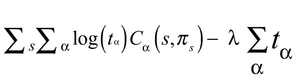(5)

for a Lagrange multiplier λ, has the closed-form solution

$$t_{\alpha }^{\text{*}}=\frac{{{\displaystyle \sum }}_s{C}_{\alpha }(s,{\pi }_s)}{{{\displaystyle \sum }}_s{{\displaystyle \sum }}_{{\alpha }^{\text{'}}}{C}_{{\alpha }^{\text{'}}}(s,{\pi }_s)}$$ (6)

that is, the ML estimation of probabilistic parameters corresponds to taking the total frequency of occurrence of features in the training set.

ML parameterization alone is problematic when data are scarce, because some parameters will get zero values, thus overfitting to the data. One usually adds priors to the ML estimates (for instance, a +1 pseudocount for each feature as in the Laplace priors). Estimations of probabilities adding priors correspond to a posterior mean estimate of the parameters under a Bayesian interpretation.

ML optimization cannot be applied to a weights scoring scheme because those are discriminative methods which can only calculate the conditional probability of structures given a sequence. One of the most widely used training methods for discriminative methods is conditional maximum likelihood (CML). CML estimation of the weights is done by optimizing for a training set the quantity ∑_Slog P(π_s | s, D). There is not a closed-form solution for such optimization problem due to the normalization term in the denominator of Eq. 2. One needs to use numerical optimization techniques to obtain the CML trained parameters, for example as in CONTRAfold.³¹ In reference 34, the authors propose architectures that match different versions of the nearest-neighbor thermodynamic model, and then use the thermodynamic parameters as input in the optimization process. All these CML training methods are usually quite time consuming since they require global optimizations for the whole training set. Alternative faster methods for CML training that do not require such global optimization (“online” training) have been devised,^54,55 and applied for RNA structure prediction.³⁵ Using test sets with substantial structural diversity with respect to the training set suggests that the online training methods are particularly vulnerable to overtraining (see Table 1).

Obviously, a generative model can also be trained by CML since from the joint distribution in Eq. 1, one can always calculate the conditional probability in Eq. 2 (although not the other way around). Not many results have been reported for this type of training for RNA probabilistic methods. Additionally, generative methods can be trained using expectation-maximization (EM) techniques or Gibbs sampling and Markov chain Monte Carlo (MCMC) methods which do not require to know a trusted secondary structure of the RNA sequences in the training set.⁴³ EM training could be useful if there are not well-trusted structures for known structural RNAs. A few methods have reported implementing EM training for RNA folding.^21,25,56

Selection of training sets

The success of a given training method depends critically on the selection of an adequate training set. Some important limitations of the data sets of structural RNAs currently used for training have been recently pointed out.³⁹

Early statistical methods like Pfold trained the parameters of the model from tRNAs (tRNAs) and large subunit rRNAs (LSU rRNA). The pre-QRNA and QRNA SCFGs were trained using tRNAs and small subunit rRNAs (SSU rRNA),^23,24 and the simple grammars in reference 30 were trained using small and large subunit rRNAs. Notice that all those methods together account for only three different RNA structures used for training. The advent of statistical models with larger number of parameters required using more structurally diverse training sets. For CONTRAfold, the authors devised a collection of 151 different structures from Rfam (S-151Rfam).³¹ This training set is structurally diverse but the number of actual sequences is small. CONTRAfold has a relatively small number of parameters (about 300), which made its training on S-151Rfam successful. When Andronescu et al. started training grammars with several thousands of parameters compatible with the nearest-neighbor thermodynamic model, they devised a large set of known RNA structures taken from different reliable sources.^57-62 The Andronescu data sets (which come under different names as they have evolved in time: S-Processed-TRA/TES,³³ RNA STRAND v2.0⁴⁰ and S-Full-Train/Test³⁴) are currently the most widely used sets of RNA structures for training and testing performance of new methods. Still the Andronescu data set, while containing on the order of 3,000 sequences, covers only six different RNA structures: small and large subunit rRNAs, tRNAs, tmRNAs, ribonuclease P RNA and signal recognition particle RNAs.

In order to benchmark methods for RNA secondary structure prediction, one needs to test performance on structural RNA sequences that are dissimilar to those in the training set not just by sequence, but also by structure. This fact has been under appreciated for some time, but it has become apparent when analyzing models with large number of parameters that have used subsets of the Andronescu data set both for training and testing.³⁹ In order to be able to train and test using structurally different data sets reference 39, devised a new training/testing paradigm. The new data sets include: TrainSetA/TestSetA, which consists of a non-redundant version of the Andronescu data sets (containing six different structures), augmented with four other structures from reference 63 and TrainSetB/TestSetB structurally dissimilar to the previous, which consists of 22 different RNA structures collected from Rfam v10.0.

Most of the RNA structural diversity currently available comes from sequences collected from the Rfam database. Those structures are problematic since they are oftentimes just predictions, and by construction they are consensus structures for an alignment of the RNA family, not individual sequence structures. An advance for single-sequence RNA secondary structure prediction will likely come as the number of crystallized structurally different individual RNA structures increases, and training of these models improves.

Folding Algorithms

Unlike the training algorithms, which are specific for the different scoring schemes, the folding algorithms are essentially identical for all scoring schemes. Thus, one can talk about different structure prediction algorithms independently of the scoring system. For example, in the generalized grammar method TORNADO³⁹ the exact same C functions are used when an architecture is given a thermodynamic parameterization that reproduces the results of the ViennaRNA package, and when the same architecture is given a probabilistic parameterization trained on a data set of RNA structures. One just needs to replace in the algorithms the thermodynamic scores with the logarithm of the corresponding probability parameters, or with the weights of a statistical discriminative method.

The most widely used folding algorithms fall in the category of “dynamic programming” (DP) algorithms. These algorithms assume that the RNA structure is additive (which will be true for any CFG). Additivity allows the DP algorithms to achieve optimality with a computational complexity of O(l³) in time and O(l²) in memory, for a sequence of length l. In principle, complex nearest-neighbor architectures can require O(l⁴) in time, but under certain simplifying assumptions,⁶⁴ or by simply fixing a maximal length for internal loops (in most current implementations 30 nucleotides), it is usually brought back to O(l³), which is already quite taxing for everyday use with long sequences.

The first dynamic programming algorithms for RNA secondary structure prediction were introduced even before the advent of the nearest-neighbor model,^1,65 and they were almost immediately applied to the nearest-neighbor model.^2,3 The prominence of DP algorithms is such that several specific programming languages have been devised in order to facilitate the fast and automatic description of such algorithms for a variety of either RNA CFG architectures³⁹ and others.^66-69

The main dynamic programming algorithms used in RNA secondary structure prediction are:

The optimal structure: This dynamic programming calculates the best scoring structure given the sequence and the model. In a thermodynamic parameterization, it calculates the minimum free-energy structure, and it is referred to as the MFE algorithm. In a probabilistic implementation, it calculates the structure with the highest probability, and it is named the Cocke-Younger-Kasami (CYK) algorithm.^70-72 The MFE and CYK algorithms are essentially the same algorithm.

The partition function or probability of the RNA: Given an RNA sequence, one can integrate the contribution of all structures allowed by the model. In a thermodynamic parameterization requires assigning a Boltzmann factor to each structure, and summing them all into what is referred to as the partition function. In a probabilistic implementation, it simply requires summing the probabilities of all possible structures.

The McCaskill algorithm is a DP algorithm that was introduced to effectively calculate the thermodynamic partition function,⁷³ and it is closely related to the inside (and outside) algorithms used for a SCFG to calculate the probability of the RNA summing to all possible structures.^74,75 These algorithms have the same time and memory complexity as the simpler optimal structure algorithms namely, O(l³) in time and O(l²) in memory for a sequence of length l.

Posterior probabilities of basepairs: Using the partition function or the inside/outside algorithms, one can calculate the posterior probabilities that any two bases in the sequence form a basepair. These basepair probabilities are named “posterior” because the basepair potential of any two bases is inferred by taking into account the overall folding potential of the rest of the RNA.

Using the McCaskill/inside algorithm one can also sample structures from the Boltzmann ensemble or posterior distribution of structures given a sequence. This is useful for studying possible alternative structures for a given RNA.⁷⁶ For this problem, there is an algorithm that samples rigorously and exactly from the distribution of structures.^43,77,78 Dynamic programming algorithms have also been proposed to calculate other posterior probabilities behond basepair interactions such as triplet interactions.⁷⁹

Maximal expected accuracy (MEA) structure: Using the posterior probabilities of basepairs, one can infer a point estimate of a plausible structure such that it maximizes the total posterior probability of basepairs. This kind of methods were first introduced in sequence analysis for alignment algorithms,⁸⁰ later applied to hidden Markov models⁸¹ and first used for RNA secondary structure in the method Pfold.²²

Since then, different MEA estimators have been implemented for RNA folding, either by maximizing the posterior probabilities of basepairs,^22,31 or calculating centroid estimators.^36,82 Reference 21 optimizes ∑ P_ij, where P_ij the posterior probability of forming a basepair between positions i and j. Reference 31 optimizes the quantity,

$$\gamma \frac{P_{ij}}{P_i{P}_j}$$

where P_iis the posterior probability of position i being single stranded, and γ a positive tunable parameter, I refer to this method as c-MEA (for CONTRAfold-MEA). Reference 36 optimizes the sum of posterior probabilities such that

,$$Pij\ge \frac{1}{1+\gamma }$$

which is a generalization of the centroid estimator in reference 82, which corresponds to the particular case γ = 1. These γ-centroid estimators are often referred to as generalized centroid estimators (GCE). All MEA methods (except for the simpler γ = 1 centroid), require to perform another dynamic programming calculation (with same time and memory requirements than other RNA DP algorithms) to obtain the optimal point-estimate MEA structure from the distribution of all possible structures.

In terms of performance, all MEA methods perform somewhat better than the simpler CYK method. Among all the MEA methods, those with a tunable parameter^31,36 are superior to those that do not have that feature.^22,82 Different MEA methods with a tunable parameter perform comparably to each other.³⁹ These improvements of MEA over CYK algorithms occur consistently across all three different scoring systems, and have been documented for several different actual parameterizations.³⁶ Currently, most RNA folding packages use a MEA estimator to predict RNA structures.⁶³ For that reason, when comparing the performance of different methods, it is important to use the same folding algorithm otherwise the differences will be reflecting the differences in the folding algorithms rather than the differences in the models’ features.

Discussion

With all these possible methods with large number of parameters, alternative scoring schemes, different statistical parameterizations, and more powerful folding algorithms, what is the state of the art for single-sequence RNA secondary structure prediction?

Using methods like TORNADO³⁹ and others,⁸³ there has been an extensive exploration of RNA grammar architectures that go even beyond the complexities of the nearest-neighbor model. However, the performance of these more complex architectures and alternative scoring systems is not dramatically better than already existing ones. A method has also been proposed (named hierarchical Dirichlet process for SCFGs) in which the architecture of the model is not fixed a priori but optimally inferred in view of the training set. The idea is quite exciting, but results again seem to be comparable to those of other methods.⁸⁴

A representative (but by no means comprehensive) summary of the current situation of different RNA single-sequence secondary structure prediction methods is given in Table 1. One observation is that thermodynamic methods are outperformed by statistical methods (both probabilistic and weighted) with comparable number of parameters. A comparison between methods ViennaRNA v1.8.4 and ViennaRNAG is a direct measure of the different performance of the same architecture under a thermodynamic or probabilistic parameterizations. Similarly, a comparison between CONTRAfold v2.02 and CONTRAfoldG is a direct measure of the differences between the same architecture under a weighted and probabilistic parameterization respectively. In both cases, the probabilistic parameterization performs better, but the differences are not large (especially for the two CONTRAfold statistical models).

Another observation from Table 1 is that features that have been considered fundamental by the thermodynamical methods seem to have a small effect in performance accuracy. For instance, they model basic grammar while maintaining the same basic architecture than the nearest-neighbor model, does not include basepair stacking or mismatches, and the number of total parameters is significantly lower than in any thermodynamic implementation. However, basic grammar under a probabilistic scoring system performs better than the thermodynamic methods tested in Table 1. It would be interesting to obtain a thermodynamic parameterization for this CFG.

Models with complex architectures and using probabilistic scoring systems show the highest accuracy among all models tested. However, the best performance achieved is barely around 60% for the F measure. (F is defined as the harmonic mean of sensitivity and positive predictive value.) There seems to be a barrier that prevents achieving higher performance without the risks of overfitting, as can be seen in Table 1 with regard to the method ContextFold, when comparing its performance for both data sets (the data set used to train ContextFold is structurally similar to TestSetA). A dedicated effort to crystallize and to compile reliable secondary structures for more diverse RNA structures would definitely improve the overfitting training problem for large architectures, but how much improvement that would produce remains to be seen.

Single-sequence RNA secondary structure prediction is to some extent an exercise performed while holding one hand behind one’s back. When possible, one should always use complementary sources of information.

Some leverage has come in recent years by incorporating experimental information such as nucleotide-resolution selective hydroxyl acylation analyzed by primer extension (SHAPE) into methods for RNA folding.^85-89 Another promising source of information consists of the emerging patterns of covariation for non-canonical types of basepairs.⁹⁰ There is a very active are of research about RNA tertiary motifs.⁹¹ Current methods seem to go in the direction of profiling and cataloging the different types of motifs,^92-96 or can only be used to predict the structure of very small RNA sequences.⁴⁹

I would advocate that at the moment, comparative analysis (at the structural/sequence level) is the most powerful method for characterizing new structural RNAs and inferring their structure. In the presence of a novel RNA, one can use any of the single-sequence methods to have a proposed secondary structure. Using close relatives, it is very likely these days to obtain similar sequences by sequence-only comparative analysis. In that situation, one should use the much more powerful profile structural comparative methods^28,97 in order to build a consensus structure for all homolog sequences. One can also use the profile model to search for other more distant candidates, which in turn will help refining the structure of the RNA. Representative examples of this approach are given in references 98 and 99.

Disclosure of Potential Conflicts of Interest

No potential conflicts of interest were disclosed.

Funding

This work is supported by the Howard Hughes Medical Institute.

References

- 1.Nussinov R, Pieczenik G, Griggs JR, Kleitman DJ. Algorithms for loop matchings. SIAM J Appl Math. 1978;35:68–82. doi: 10.1137/0135006. [DOI] [Google Scholar]
- 2.Waterman MS, Smith TF. RNA secondary structure: A complete mathematical analysis. Math Biosci. 1978;42:257–66. doi: 10.1016/0025-5564(78)90099-8. [DOI] [Google Scholar]
- 3.Zuker M, Stiegler P. Optimal computer folding of large RNA sequences using thermodynamics and auxiliary information. Nucleic Acids Res. 1981;9:133–48. doi: 10.1093/nar/9.1.133. [DOI] [PMC free article] [PubMed] [Google Scholar]
- 4.Zuker M, Sankoff S. RNA secondary structures and their prediction. Bull Math Biol. 1984;46:591–621. [Google Scholar]
- 5.Tinoco I, Jr., Uhlenbeck OC, Levine MD. Estimation of secondary structure in ribonucleic acids. Nature. 1971;230:362–7. doi: 10.1038/230362a0. [DOI] [PubMed] [Google Scholar]
- 6.Freier SM, Kierzek R, Jaeger JA, Sugimoto N, Caruthers MH, Neilson T, et al. Improved free-energy parameters for predictions of RNA duplex stability. Proc Natl Acad Sci USA. 1986;83:9373–7. doi: 10.1073/pnas.83.24.9373. [DOI] [PMC free article] [PubMed] [Google Scholar]
- 7.Turner DH, Sugimoto N, Jaeger JA, Longfellow CE, Freier SM, Kierzek R. Improved parameters for prediction of RNA structure. Cold Spring Harb Symp Quant Biol. 1987;52:123–33. doi: 10.1101/SQB.1987.052.01.017. [DOI] [PubMed] [Google Scholar]
- 8.Kim J, Walter AE, Turner DH. Thermodynamics of coaxially stacked helixes with GA and CC mismatches. Biochemistry. 1996;35:13753–61. doi: 10.1021/bi960913z. [DOI] [PubMed] [Google Scholar]
- 9.Xia T, Jr SantaLucia J, Burkard ME, Kierzek R, Schroeder SJ. X. Jiao anc C. Cox, and D. H. Turner. Thermodynamic parameters for an expanded nearest-neighbor model for formation of RNA duplexes with Watson-Crick base pairs. Biochemestry. 1998;37:14719–35. doi: 10.1021/bi9809425. [DOI] [PubMed] [Google Scholar]
- 10.Mathews DH, Andre TC, Kim J, Turner DH, Zuker M. An updated recursive algorithm for RNA secondary structure prediction with improved thermodynamic parameters. In N. B. Leontis and J. Jr Santalucia, editors, Molecular Modeling of Nucleic Acids, pages 246–257. American Chemical Society, 1998. [Google Scholar]
- 11.Mathews DH, Sabina J, Zuker M, Turner DH. Expanded sequence dependence of thermodynamic parameters improves prediction of RNA secondary structure. J Mol Biol. 1999;288:911–40. doi: 10.1006/jmbi.1999.2700. [DOI] [PubMed] [Google Scholar]
- 12.Liu B, Diamond JM, Mathews DH, Turner DH. Fluorescence competition and optical melting measurements of RNA three-way multibranch loops provide a revised model for thermodynamic parameters. Biochemistry. 2011;50:640–53. doi: 10.1021/bi101470n. [DOI] [PMC free article] [PubMed] [Google Scholar]
- 13.Zuker M. Mfold web server for nucleic acid folding and hybridization prediction. Nucleic Acids Res. 2003;31:3406–15. doi: 10.1093/nar/gkg595. [DOI] [PMC free article] [PubMed] [Google Scholar]
- 14.Markham NR, Zuker M. UNAFold: software for nucleic acid folding and hybriziation. In J. M. Keith, editor, Bioinformatics, Volume II. Structure, Function and Applications, chapter 1, pages 3–31. Humana Press, Totowa, NJ, 2008. [Google Scholar]
- 15.Hofacker IL, Fontana W, Stadler PF, Bonhoeffer LS, Tacker M, Schuster P. Fast folding and comparison of RNA secondary structures (the Vienna RNA package) Monatsh Chem. 1994;125:167–88. doi: 10.1007/BF00818163. [DOI] [Google Scholar]
- 16.Lorenz R, Bernhart SH, Höner Zu Siederdissen C, Tafer H, Flamm C, Stadler PF, et al. ViennaRNA Package 2.0. Algorithms Mol Biol. 2011;6:26. doi: 10.1186/1748-7188-6-26. [DOI] [PMC free article] [PubMed] [Google Scholar]
- 17.Reuter JS, Mathews DH. RNAstructure: software for RNA secondary structure prediction and analysis. BMC Bioinformatics. 2010;11:129. doi: 10.1186/1471-2105-11-129. [DOI] [PMC free article] [PubMed] [Google Scholar]
- 18.Konings DAM, Gutell RR. A comparison of thermodynamic foldings with comparatively derived structures of 16S and 16S-like rRNAs. RNA. 1995;1:559–74. [PMC free article] [PubMed] [Google Scholar]
- 19.Doshi KJ, Cannone JJ, Cobaugh CW, Gutell RR. Evaluation of the suitability of free-energy minimization using nearest-neighbor energy parameters for RNA secondary structure prediction. BMC Bioinformatics. 2004;5:105. doi: 10.1186/1471-2105-5-105. [DOI] [PMC free article] [PubMed] [Google Scholar]
- 20.Gardner PP, Giegerich R. A comprehensive comparison of comparative RNA structure prediction approaches. BMC Bioinformatics. 2004;5:140. doi: 10.1186/1471-2105-5-140. [DOI] [PMC free article] [PubMed] [Google Scholar]
- 21.Grate L, Herbster M, Hughey R, Haussler D, Mian IS, Noller H. RNA modeling using Gibbs sampling and stochastic context free grammars. ISMB proceedings, pages 138–146, 1994. [PubMed] [Google Scholar]
- 22.Knudsen B, Hein J. RNA secondary structure prediction using stochastic context-free grammars and evolutionary history. Bioinformatics. 1999;15:446–54. doi: 10.1093/bioinformatics/15.6.446. [DOI] [PubMed] [Google Scholar]
- 23.Rivas E, Eddy SR. Secondary structure alone is generally not statistically significant for the detection of noncoding RNAs. Bioinformatics. 2000;16:583–605. doi: 10.1093/bioinformatics/16.7.583. [DOI] [PubMed] [Google Scholar]
- 24.Rivas E, Eddy SR. Noncoding RNA gene detection using comparative sequence analysis. BMC Bioinformatics. 2001;2:8. doi: 10.1186/1471-2105-2-8. [DOI] [PMC free article] [PubMed] [Google Scholar]
- 25.Eddy SR, Durbin R. RNA sequence analysis using covariance models. Nucleic Acids Res. 1994;22:2079–88. doi: 10.1093/nar/22.11.2079. [DOI] [PMC free article] [PubMed] [Google Scholar]
- 26.Sakakibara Y, Brown M, Hughey R, Mian IS, Sjölander K, Underwood RC, et al. Stochastic context-free grammars for tRNA modeling. Nucleic Acids Res. 1994;22:5112–20. doi: 10.1093/nar/22.23.5112. [DOI] [PMC free article] [PubMed] [Google Scholar]
- 27.Knudsen B, Hein J. Pfold: RNA secondary structure prediction using stochastic context-free grammars. Nucleic Acids Res. 2003;31:3423–8. doi: 10.1093/nar/gkg614. [DOI] [PMC free article] [PubMed] [Google Scholar]
- 28.Nawrocki EP, Kolbe DL, Eddy SR. Infernal 1.0: inference of RNA alignments. Bioinformatics. 2009;25:1335–7. doi: 10.1093/bioinformatics/btp157. [DOI] [PMC free article] [PubMed] [Google Scholar]
- 29.Pedersen JS, Meyer IM. R. Forsberg R, P. Simmonds, and J. Hein. A comparative method for finding and folding RNA secondary structures within protein-coding regions. Nucleic Acids Res. 2004;24:4925–36. doi: 10.1093/nar/gkh839. [DOI] [PMC free article] [PubMed] [Google Scholar]
- 30.Dowell RD, Eddy SR. Evaluation of several lightweight stochastic context-free grammars for RNA secondary structure prediction. BMC Bioinformatics. 2004;5:71. doi: 10.1186/1471-2105-5-71. [DOI] [PMC free article] [PubMed] [Google Scholar]
- 31.Do CB, Woods DA, Batzoglou S. CONTRAfold: RNA secondary structure prediction without physics-based models. Bioinformatics. 2006;22:e90–8. doi: 10.1093/bioinformatics/btl246. [DOI] [PubMed] [Google Scholar]
- 32.Do CB, Foo CS, Ng AY. Efficient multiple hyperparameter learning for log-linear models. In Advances in Neural Information Processing Systems, volume 20, pages 377–384. MIT press, Cambridge, MA, 2007. [Google Scholar]
- 33.Andronescu M, Condon A, Hoos HH, Mathews DH, Murphy KP. Efficient parameter estimation for RNA secondary structure prediction. Bioinformatics. 2007;23:i19–28. doi: 10.1093/bioinformatics/btm223. [DOI] [PubMed] [Google Scholar]
- 34.Andronescu M, Condon A, Hoos HH, Mathews DH, Murphy KP. Computational approaches for RNA energy parameter estimation. RNA. 2010;16:2304–18. doi: 10.1261/rna.1950510. [DOI] [PMC free article] [PubMed] [Google Scholar]
- 35.Zakov S, Goldberg Y, Elhadad M, Ziv-Ukelson M. Rich parameterization improves RNA structure prediction. In V. Bafna and S. C. Sahinalp, editors, RECOMB 2011, LNBI 6577, pages 546–562. Springer–Verlag, 2011. [DOI] [PubMed] [Google Scholar]
- 36.Hamada M, Kiryu H, Sato K, Mituyama T, Asai K. Prediction of RNA secondary structure using generalized centroid estimators. Bioinformatics. 2009;25:465–73. doi: 10.1093/bioinformatics/btn601. [DOI] [PubMed] [Google Scholar]
- 37.Weinberg F, Nebel ME. Extending stochastic context-free grammars for an application in bioinformatics. In Language and Automata Theory and Applications. Lecture Notes in Computer Science, volume 6031, pages 585–595, 2010. [Google Scholar]
- 38.Nebel ME, Scheid A. Evaluation of a sophisticated SCFG design for RNA secondary structure prediction. Theory Biosci. 2011;130:313–36. doi: 10.1007/s12064-011-0139-7. [DOI] [PubMed] [Google Scholar]
- 39.Rivas E, Lang R, Eddy SR. A range of complex probabilistic models for RNA secondary structure prediction that includes the nearest-neighbor model and more. RNA. 2012;18:193–212. doi: 10.1261/rna.030049.111. [DOI] [PMC free article] [PubMed] [Google Scholar]
- 40.Andronescu M. Computational approaches for RNA energy parameter estimation. PhD thesis, Department of Computer Science, University of British Columbia, Vancouver, BC, Canada., 2008. [Google Scholar]
- 41.Chomsky N. On certain formal properties of grammars. Inf Control. 1959;2:137–67. doi: 10.1016/S0019-9958(59)90362-6. [DOI] [Google Scholar]
- 42.Leontis NB, Westhof E. Geometric nomenclature and classification of RNA base pairs. RNA. 2001;7:499–512. doi: 10.1017/S1355838201002515. [DOI] [PMC free article] [PubMed] [Google Scholar]
- 43.Durbin R, Eddy SR, Krogh A, Mitchison GJ. Biological Sequence Analysis: Probabilistic Models of Proteins and Nucleic Acids Cambridge University Press, Cambridge UK, 1998. [Google Scholar]
- 44.Hopcroft JE, Ullman JD. Introduction to Automata Theory, Languages, and Computation Addison-Wesley, Reading, Massachusetts, 1979. [Google Scholar]
- 45.Giegerich R. Explaining and controlling ambiguity in dynamic programming. In R. Giancarlo and D. Sankoff, editors, Proceedings of the 11th Annual Symposium on Combinatorial Pattern Matching, number 1848, pages 46–59, Montréal, Canada, 2000. Springer-Verlag, Berlin. [Google Scholar]
- 46.Höner zu Siederdissen C, Bernhart SH, Stadler PF, Hofacker IL. A folding algorithm for extended RNA secondary structures. Bioinformatics. 2011;27:i129–36. doi: 10.1093/bioinformatics/btr220. [DOI] [PMC free article] [PubMed] [Google Scholar]
- 47.Rivas E, Eddy SR. A dynamic programming algorithm for RNA structure prediction including pseudoknots. J Mol Biol. 1999;285:2053–68. doi: 10.1006/jmbi.1998.2436. [DOI] [PubMed] [Google Scholar]
- 48.Dirks RM, Pierce NA. An algorithm for computing nucleic acid base-pairing probabilities including pseudoknots. J Comput Chem. 2004;25:1295–304. doi: 10.1002/jcc.20057. [DOI] [PubMed] [Google Scholar]
- 49.Parisien M, Major F. The MC-Fold and MC-Sym pipeline infers RNA structure from sequence data. Nature. 2008;452:51–5. doi: 10.1038/nature06684. [DOI] [PubMed] [Google Scholar]
- 50.Johnson M. Joint and conditional estimation of tagging and parsing models. In Proceedings of the Association for Computational Linguistics (ACL), Toulouse, France., 2001. Morgan Kaufmann Publishers. [Google Scholar]
- 51.Ng AY, Jordan MI. On discriminative vs. generative classifiers: A comparison of logistic regression and naive Bayes. In T. Dietterich, S. Becker, and Z. Ghahramani, editors, Advances in Neural Information Processing Systems (NIPS), volume 14, pages 841–848, Cambridge, MA, 2002. MIT Press. [Google Scholar]
- 52.Liang P, Jordan MI. An analysis of generative, discriminative, and pseudolikelihood estimators. In Proceedings of the 25th International Conference on Machine Learning (ICML), Helsinki, Finland, 2008. Omnipress. [Google Scholar]
- 53.Dima RI, Hyeon C, Thirumalai D. Extracting stacking interaction parameters for RNA from the data set of native structures. J Mol Biol. 2005;347:53–69. doi: 10.1016/j.jmb.2004.12.012. [DOI] [PubMed] [Google Scholar]
- 54.Kivinen J, Smola AJ, Williamson RC. Online learning with kernels. Signal Processing, IEEE. 2004;52:2165–76. doi: 10.1109/TSP.2004.830991. [DOI] [Google Scholar]
- 55.Crammer K, Dekel O, Keshet J, Shalev-Shwartz S, Singer Y. Online passive-aggressive algorithms. J Mach Learn Res. 2006;7:551–85. [Google Scholar]
- 56.Kin T, Tsuda K, Asai K. Marginalized kernels for RNA sequence data analysis. Genome Inform. 2002;13:112–22. [PubMed] [Google Scholar]
- 57.Cannone JJ, Subramanian S, Schnare MN, Collett JR, D’Souza LM, Du Y, et al. The comparative RNA web (CRW) site: an online database of comparative sequence and structure information for ribosomal, intron, and other RNAs. BMC Bioinformatics. 2002;3:2. doi: 10.1186/1471-2105-3-2. [DOI] [PMC free article] [PubMed] [Google Scholar]
- 58.Sprinzl M, Vassilenko KS. Compilation of tRNA sequences and sequences of tRNA genes. Nucleic Acids Res. 2005;33:139–40. doi: 10.1093/nar/gki012. [DOI] [PMC free article] [PubMed] [Google Scholar]
- 59.Andersen ES, Rosenblad MA, Larsen N, Westergaard JC, Burks J, Wower IK, et al. The tmRDB and SRPDB resources. Nucleic Acids Res. 2006;34(Database issue):D163–8. doi: 10.1093/nar/gkj142. [DOI] [PMC free article] [PubMed] [Google Scholar]
- 60.Brown JW. The ribonuclease P database. Nucleic Acids Res. 1999;27:314. doi: 10.1093/nar/27.1.314. [DOI] [PMC free article] [PubMed] [Google Scholar]
- 61.Berman HM, Olson WK, Beveridge DL, Westbrook J, Gelbin A, Demeny T, et al. The nucleic acid database. A comprehensive relational database of three-dimensional structures of nucleic acids. Biophys J. 1992;63:751–9. doi: 10.1016/S0006-3495(92)81649-1. [DOI] [PMC free article] [PubMed] [Google Scholar]
- 62.Westbrook J, Feng Z, Chen L, Yang H, Berman HM. The protein data bank and structural genomics. Nucleic Acids Res. 2003;31:489–91. doi: 10.1093/nar/gkg068. [DOI] [PMC free article] [PubMed] [Google Scholar]
- 63.Lu ZJ, Gloor JW, Mathews DH. Improved RNA secondary structure prediction by maximizing expected pair accuracy. RNA. 2009;15:1805–13. doi: 10.1261/rna.1643609. [DOI] [PMC free article] [PubMed] [Google Scholar]
- 64.Lyngsø RB, Zuker M, Pedersen CNS. Fast evaluation of internal loops in RNA secondary structure prediction. Bioinformatics. 1999;15:440–5. doi: 10.1093/bioinformatics/15.6.440. [DOI] [PubMed] [Google Scholar]
- 65.Waterman MS. Secondary structure of single stranded nucleic acids. Adv Math Suppl Stud. 1978:167–212. [Google Scholar]
- 66.Giegerich R, Steffen P. Challenges in the compilation of domain specific language for dynamic programming. In Proceedings of the 2006 ACM symposium on applied computing, New York, 2006. Association for computing machine (ACM). [Google Scholar]
- 67.Goodman ND, Mansighka VK, Roy D, Bonawitz K, Tenenbaum JB. Church, a language for generative models. In Uncertainty in Artificial Intelligence, Arlington, Virginia, 2008. AUAI Press. [Google Scholar]
- 68.Sauthoff G, Möhl M, Janssen S, Giegerich R. Bellman’s GAP--a language and compiler for dynamic programming in sequence analysis. Bioinformatics. 2013;29:551–60. doi: 10.1093/bioinformatics/btt022. [DOI] [PMC free article] [PubMed] [Google Scholar]
- 69.Höner zu Siederdissen C. Sneaking around concatMap: efficient combinators for dynamic programming. Proceedings of the 17th ACM SIGPLAN, 2012. [Google Scholar]
- 70.Kasami T. An efficient recognition and syntax algorithm for context-free algorithms. Technical Report AFCRL-65-758, Air Force Cambridge Research Lab, Bedford, Mass., 1965.
- 71.Younger DH. Recognition and parsing of context-free languages in time. Inf Control. 1967;10:189–208. doi: 10.1016/S0019-9958(67)80007-X. [DOI] [Google Scholar]
- 72.Cocke J, Schwartz JT. Programming languages and their compilers: Preliminary notes. Technical report, Courant Institute of Mathematical Sciences, New York University, 1970. [Google Scholar]
- 73.McCaskill JS. The equilibrium partition function and base pair binding probabilities for RNA secondary structure. Biopolymers. 1990;29:1105–19. doi: 10.1002/bip.360290621. [DOI] [PubMed] [Google Scholar]
- 74.Lari K, Young SJ. The estimation of stochastic context-free grammars using the inside-outside algorithm. Comput Speech Lang. 1990;4:35–56. doi: 10.1016/0885-2308(90)90022-X. [DOI] [Google Scholar]
- 75.Lari K, Young SJ. Applications of stochastic context-free grammars using the inside-outside algorithm. Comput Speech Lang. 1991;5:237–57. doi: 10.1016/0885-2308(91)90009-F. [DOI] [Google Scholar]
- 76.Wuchty S, Fontana W, Hofacker IL, Schuster P. Complete suboptimal folding of RNA and the stability of secondary structures. Biopolymers. 1999;49:145–65. doi: 10.1002/(SICI)1097-0282(199902)49:2<145::AID-BIP4>3.0.CO;2-G. [DOI] [PubMed] [Google Scholar]
- 77.Ding Y, Lawrence CE. A statistical sampling algorithm for RNA secondary structure prediction. Nucleic Acids Res. 2003;31:7280–301. doi: 10.1093/nar/gkg938. [DOI] [PMC free article] [PubMed] [Google Scholar]
- 78.Kiryu H, Kin T, Asai K. Rfold: an exact algorithm for computing local base pairing probabilities. Bioinformatics. 2008;24:367–73. doi: 10.1093/bioinformatics/btm591. [DOI] [PubMed] [Google Scholar]
- 79.Miklós I, Meyer IM, Nagy B. Moments of the Boltzmann distribution for RNA secondary structures. Bull Math Biol. 2005;67:1031–47. doi: 10.1016/j.bulm.2004.12.003. [DOI] [PubMed] [Google Scholar]
- 80.Miyazawa S. A reliable sequence alignment method based on probabilities of residue correspondences. Protein Eng. 1995;8:999–1009. doi: 10.1093/protein/8.10.999. [DOI] [PubMed] [Google Scholar]
- 81.Holmes I. Studies in Probabilistic Sequence Alignment and Evolution PhD thesis, University of Cambridge, 1998. [Google Scholar]
- 82.Ding Y, Chan CY, Lawrence CE. RNA secondary structure prediction by centroids in a Boltzmann weighted ensemble. RNA. 2005;11:1157–66. doi: 10.1261/rna.2500605. [DOI] [PMC free article] [PubMed] [Google Scholar]
- 83.Anderson JWJ, Tataru P, Staines J, Hein J, Lyngsø R. Evolving stochastic context-free grammars for RNA secondary structure prediction. BMC Bioinformatics. 2012;13:78. doi: 10.1186/1471-2105-13-78. [DOI] [PMC free article] [PubMed] [Google Scholar]
- 84.Sato K, Hamada M, Mituyama T, Asai K, Sakakibara Y. A non-parametric Bayesian approach for predicting RNA secondary structures. J Bioinform Comput Biol. 2010;8:727–42. doi: 10.1142/S0219720010004926. [DOI] [Google Scholar]
- 85.Deigan KE, Li TW. D. H. Mathews DH, and K. M. Weeks. Accurate SHAPE-directed RNA structure determination. Proc Natl Acad Sci USA. 2009;6:97–102. doi: 10.1073/pnas.0806929106. [DOI] [PMC free article] [PubMed] [Google Scholar]
- 86.Washietl S, Hofacker IL, Stadler PF, Kellis M. RNA folding with soft constraints: reconciliation of probing data and thermodynamic secondary structure prediction. Nucleic Acids Res. 2012;40:4261–72. doi: 10.1093/nar/gks009. [DOI] [PMC free article] [PubMed] [Google Scholar]
- 87.Hamada M. Direct updating of an RNA base-pairing probability matrix with marginal probability constraints. J Comput Biol. 2012;19:1265–76. doi: 10.1089/cmb.2012.0215. [DOI] [PMC free article] [PubMed] [Google Scholar]
- 88.Sükösd Z, Knudsen B, Vaerum M, Kjems J, Andersen ES. Multithreaded comparative RNA secondary structure prediction using stochastic context-free grammars. BMC Bioinformatics. 2011;12:103. doi: 10.1186/1471-2105-12-103. [DOI] [PMC free article] [PubMed] [Google Scholar]
- 89.Sükösd Z, Knudsen B, Kjems J, Pedersen CNS. PPfold 3.0: fast RNA secondary structure prediction using phylogeny and auxiliary data. Bioinformatics. 2012;28:2691–2. doi: 10.1093/bioinformatics/bts488. [DOI] [PubMed] [Google Scholar]
- 90.Stombaugh J, Zirbel CL, Westhof E, Leontis NB. Frequency and isostericity of RNA base pairs. Nucleic Acids Res. 2009;37:2294–312. doi: 10.1093/nar/gkp011. [DOI] [PMC free article] [PubMed] [Google Scholar]
- 91.Leontis NB, Westhof E. Analysis of RNA motifs. Curr Opin Struct Biol. 2003;13:300–8. doi: 10.1016/S0959-440X(03)00076-9. [DOI] [PubMed] [Google Scholar]
- 92.Wang JTL, Wen D, Shapiro BA, Herbert KG, Li J, Ghosh K. Toward an integrated RNA motif database. DILS’07 Proceedings of the 4th international conference on Data integration in the life sciences, pages 27–36, 2007. [Google Scholar]
- 93.Bindewald E, Hayes R, Yingling YG, Kasprzak W, Shapiro BA, Junction BARNA. RNAJunction: a database of RNA junctions and kissing loops for three-dimensional structural analysis and nanodesign. Nucleic Acids Res. 2008;36(Database issue):D392–7. doi: 10.1093/nar/gkm842. [DOI] [PMC free article] [PubMed] [Google Scholar]
- 94.Cruz JA, Westhof E. Sequence-based identification of 3D structural modules in RNA with RMDetect. Nat Methods. 2011;8:513–21. doi: 10.1038/nmeth.1603. [DOI] [PubMed] [Google Scholar]
- 95.Abu Almakarem AS, Petrov AI, Stombaugh J, Zirbel CL, Leontis NB. Comprehensive survey and geometric classification of base triples in RNA structures. Nucleic Acids Res. 2012;40:1407–23. doi: 10.1093/nar/gkr810. [DOI] [PMC free article] [PubMed] [Google Scholar]
- 96.Vanegas PL, Hudson GA, Davis AR, Kelly SC, Kirkpatrick CC, Znosko BM. RNA CoSSMos: Characterization of Secondary Structure Motifs--a searchable database of secondary structure motifs in RNA three-dimensional structures. Nucleic Acids Res. 2012;40(Database issue):D439–44. doi: 10.1093/nar/gkr943. [DOI] [PMC free article] [PubMed] [Google Scholar]
- 97.Lambert A, Fontaine J-F, Legendre M, Leclerc F, Permal E, Major F, et al. The ERPIN server: an interface to profile-based RNA motif identification. Nucleic Acids Res. 2004;32(suppl 2):W160-5. doi: 10.1093/nar/gkh418. [DOI] [PMC free article] [PubMed] [Google Scholar]
- 98.Jones TA, Otto W, Marz M, Eddy SR, Stadler PF. A survey of nematode SmY RNAs. RNA Biol. 2009;6:5–8. doi: 10.4161/rna.6.1.7634. [DOI] [PubMed] [Google Scholar]
- 99.del Val C, Romero-Zaliz R, Torres-Quesada O, Peregrina A, Toro N, Jiménez-Zurdo JI. A survey of sRNA families in α-proteobacteria. RNA Biol. 2012;9:119–29. doi: 10.4161/rna.18643. [DOI] [PMC free article] [PubMed] [Google Scholar]