The dual role of fragments in fragment-assembly methods for de novo protein structure prediction

Abstract

In fragment-assembly techniques for protein structure prediction, models of protein structure are assembled from fragments of known protein structures. This process is typically guided by a knowledge-based energy function and uses a heuristic optimization method. The fragments play two important roles in this process: they define the set of structural parameters available, and they also assume the role of the main variation operators that are used by the optimiser. Previous analysis has typically focused on the first of these roles. In particular, the relationship between local amino acid sequence and local protein structure has been studied by a range of authors. The correlation between the two has been shown to vary with the window length considered, and the results of these analyses have informed directly the choice of fragment length in state-of-the-art prediction techniques. Here, we focus on the second role of fragments and aim to determine the effect of fragment length from an optimization perspective. We use theoretical analyses to reveal how the size and structure of the search space changes as a function of insertion length. Furthermore, empirical analyses are used to explore additional ways in which the size of the fragment insertion influences the search both in a simulation model and for the fragment-assembly technique, Rosetta.

INTRODUCTION

Fragment-assembly techniques currently present the state-of-the-art for de novo prediction. A range of methods exist differing in the fragment size, energy functions, and optimization heuristics used. Some of the best-known methods include Fragfold,¹ Simfold² and Rosetta.³

The key idea behind fragment-assembly techniques is to take advantage of local sequence-structure correlations that can be observed in the Protein Data Bank (PDB).⁴ By using fragments from such structures as the building blocks during model construction, local propensities of the amino-acid chain are accounted for. This reduces the size of the search space. It is also thought to render the optimization less sensitive to inaccuracies in the energy function used, as local interactions are taken into account by the fragments and the energy function can focus, predominantly, on the description of nonlocal interactions.⁵

Current fragment-assembly techniques do not reliably scale to longer proteins (≥70 residues) and/or those with long-range contacts. However, it remains unclear whether the key limiting factor is the accuracy of the energy function, the effectiveness of the search heuristics, the quality of the fragment libraries used, or a combination of these three factors.^6–10 Better insight into the working mechanisms and limitations of fragment-assembly techniques will be a fundamental prerequisite for resolving this conundrum and for enabling the further improvement of these techniques.

THE DUAL ROLE OF FRAGMENTS

The relationship between local amino acid sequence and local protein structure has been studied extensively in the structural biology literature. Analysis for a range of different fragment lengths has indicated a peak in local sequence-structure correlation for an average length of 10 residues,¹¹ and this has motivated the choice of fragment length in some of the first fragment-assembly techniques.^3,12 It seems reasonable to assume that the assembly of a near-native structure from fragments becomes easier as the quality of the fragment libraries (i.e., how closely and to what proportion fragments for a given position approximate the corresponding segments of the native structure) increases, and prediction accuracy is therefore thought to be influenced directly through this route.

A range of alternative fragment-assembly methods have been developed since, and these all share core features regarding the use of fragments. Before the optimization, fragments are derived for a given window length. The resulting fragment library is then used for the construction of models in the actual optimization process, and, typically, an entire fragment is inserted at a time. There are some differences between methods regarding the window length used, and a few methods make use of several different fragment lengths.⁴

A common factor in almost all existing methods is that the fragment length(s) used also define the size(s) of the moves that are possible during the optimization (an exception to this is Profesy¹³). It is well known from the computational literature that the size and frequency with which variation operators are used can have important effects regarding the performance of a heuristic optimiser: too large or too frequent perturbation may prevent the convergence of such techniques, while too small or infrequent perturbations may impede the escape from local optima (see, e.g. Refs. ^14–17). In addition to the quality of a given fragment library, we would therefore expect the size of the moves used in a fragment-assembly method to have an important effect on the quality of the models obtained. In particular, it is possible that a fragment length that defines a fragment library of reasonable quality may be unsuitable for the use in an optimiser due to inadequacies of the move size in the context of effective optimization. Although existing methods have typically used the same fragment length during the generation of the fragment library and the actual optimization, fragment length and move size need not strictly be identical, and alternative setups are possible. Here, we differentiate between these two different roles of fragments and explore the effects of independently varying fragment length and move size. Although our focus is on the Rosetta method, the key insights are also relevant for other techniques based on fragment assembly.

METHODS

We use three different lines of investigation to illustrate the separate effects of fragment length and move size. All three of these are described in the following.

Rosetta ab initio

“Rosetta ab initio” is a fragment-assembly technique for de novo structure prediction that has performed well in the Critical Assessment of Protein Structure Prediction (CASP) experiment.¹⁸ Rosetta comprises two key protocols. The first of these is its low-resolution protocol during which coarse-grained models of protein structure are built. This is where extensive exploration of the conformational search space is taking place. The set of decoys obtained in this way are fed on to Rosetta's full-atom protocol, which attempts to refine the decoys and to identify the most promising models. Here, we are concerned with Rosetta's low resolution protocol, which is the part of the software that uses fragments as building blocks during the search.

Rosetta's low resolution protocol uses a simplified representation of a protein: side-chains are represented by their centroids and idealized bond lengths and bond angles are used. The remaining degrees of freedom are the three backbone torsion angles (φ, ψ, and ω) per amino acid. In this low resolution representation, for an amino-acid sequence of length N, a candidate structure can be unambiguously described by N angle triplets, or a string of length 3 × N.

Rosetta starts its search from the linear chain. During the optimization, Rosetta attempts to replace individual segments of the solution string by the angles of structural fragments from the PDB. A suitable library of fragments for each amino-acid position is selected before the run based on sequence profiles and secondary structure predictions for the input sequence (see Refs. ⁵ and ¹⁹ for more detail).

Here, the fragment library size F refers to the number of fragments available for insertion at a given position in the protein chain. The fragment length L ≤ N refers to the actual window length used for the generation of the fragment library.

The selection of insertion points is possible at any (but the last few) amino-acid position in the chain and fragments are allowed to overlap. In other words, the triplet of torsion angles for a given amino-acid position presents an entity, that is the three torsion angles can only take values that derive from the same fragment. In contrast, neighboring triplets may derive from completely different fragments (see Fig. 1). The only way in which continuity between neighboring residues is encouraged is through the use of fixed length fragment insertions.

Figure 1.

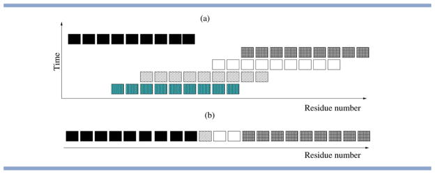
Illustration of a short stretch arising from fragment assembly using fragments of nine residues. Here, each “block” represents an angle triplet consisting of the three backbone torsions φ, ψ, and ω for a given residue. (a) Gives a temporal perspective that shows the consecutive insertion of different fragments. (b) Provides a more compact view of the relevant information. This memory-less view is adopted within most fragment-assembly techniques, that is, information about the origin and the order of insertion of given values is discarded. [Color figure can be viewed in the online issue, which is available at wileyonlinelibrary.com.]

In the following, we will use the term, angle triplet, to refer to any set of parameters {φ,ψ,ω} that derives from a specific fragment for a given position in the chain. Angle triplets are further classified into starting triplets, end triplets and central triplets, dependent on whether they derive from the first, last, or a middle position of an individual fragment.

Rosetta uses a knowledge-based energy function to score the quality of a candidate conformation. This function consists of a linear-weighted sum of 10 energy terms, which reflect different aspects of protein structures, including steric repulsion, amino-acid propensities (statistical potential), packing, and secondary structure terms. Rosetta's low resolution protocol proceeds through four different stages, as illustrated in Fig. 2. These stages differ in the weights of the energy components and the size of the fragments used.

Figure 2.

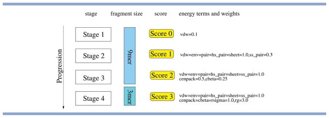
Basic structure of Rosetta's low-resolution protocol (see Ref. 5 for full details). The search progresses through four stages, which use different scoring functions. The knowledge-based scoring function combines 10 different terms, which are progressively activated (and up-weighted) as the search progresses. Stages 1–3 use fragments covering nine residues, while the last stage uses fragments covering three residues. The term vdw captures steric repulsion. The statistical potential consists of the terms env and pair, which capture the residue environment and residue pair interactions, respectively. Furthermore, there are four terms that describe interactions between secondary structure elements (ss_pair, hs_pair, sheet, and rsigma) and three terms related to the density and compactness of structures (cbeta, cenpack, and rg). See Table I in Ref. 5 for more details. [Color figure can be viewed in the online issue, which is available at wileyonlinelibrary.com.]

Rosetta only attempts a single fragment insertion at a time. Acceptance of a given insertion is decided based on the Boltzmann criterion²⁰ using a fixed temperature of T = 2. Only when Rosetta repeatedly fails to find a successful insertion (after 150 successive failed attempts), the temperature is increased temporarily, until an acceptable move has been identified.

Empirical study using a modified version of Rosetta

We define the move size M ≤ L as the size of the insertion (move operator) used during the optimization. In our experiments, M can be different from the fragment length L and we make the simplifying assumption that M ≤ L. For a given move of size M ≤ L, an actual insertion is then defined as follows (see Fig. 3).

Figure 3.

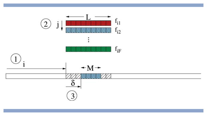
Illustration of the three key steps in performing a fragment insertion with a move size of M and a fragment size of L.(1) Select the location of the starting triplet; (2) Select the fragment from the library for that location; (3) Select the offset and insert the corresponding M angle triplets from the selected fragment. [Color figure can be viewed in the online issue, which is available at wileyonlinelibrary.com.]

1. A random position i in the chain is picked uniformly at random with 1 ≤ i ≤ N − L + 1.

2. A random fragment f_ij for position i is picked with 1 ≤ j ≤ F.

3. Within this fragment, an offset δ for the insertion is selected uniformly at random with 0 ≤ δ ≤ L − M.

4. For all positions k with i + δ ≤ k ≤ i + δ + M − 1, the corresponding angle triplets from the fragment f_ij are inserted. Hence, the length of the insertion is M.

We conduct experiments within Rosetta that are targeted at assessing directly the individual impact of move size versus that of fragment size. For this purpose, experiments are run on a benchmark set of 49 proteins (see Supporting Information). For each target protein, fragment libraries of lengths L ∈ {3,6,9,12,15,18} are generated (with homologues excluced). For a given choice of fragment library size L, we then consider different move lengths M with 3 ≤ M ≤ L. F is set to its standard value of 25. In other words, a specific fragment length L and move size M are fixed for a given run of Rosetta. For each setting of fragment length and move operator, the first two stages of Rosetta's low-resolution protocol (stage 1 and stage 2) are run 100 times and the distribution of final energies and RMSD values (across all backbone atoms) are compared using box-plots. We also relate these results to the quality of the fragment libraries. The measure used to assess the quality of individual fragments is the Euclidean distance (in torsion space) between a fragment and the corresponding section of the native structure. Boxplots are used to show the overall distribution of distances for a given fragment library where F = 25.

Markov chain analysis

Theoretical analysis is used to determine the influence of various parameters on the size and the structure of the search space. In particular, we focus on the influence of the length of a protein N, the fragment length L, the fragment library size F, and the move size M. A naive upper bound of the size of the search space can be derived using the first three parameters only: given a fragment length of L and a fragment library size of F, the number of available angle triplets at each position 1 ≤ i ≤ N is at most LF. Assuming free recombination of the triplets in these positions, a bound on the overall size of the search space is then given as S = (LF)^N. There are several reasons why this presents a very loose upper bound on the size of the search space only.

In fragment-assembly, as implemented in Rosetta, the number of available triplets decreases at both ends of the chain, due to the smaller number of fragment insertions that can affect these positions. For a fragment length L and a fragment library size F, the number of available angle triplets for position 1 ≤ i ≤ N is given as A(i) = min(L,N − L + 1,d(i)) × F, where d(i) = min(N − i + 1,i) is the distance from either end of the chain. Taking this into account, the upper bound on the size of the search space reduces from S to $S^{★}={\prod }_{i=1}^{N}A(i)$.

Furthermore, fragments for neighboring positions are likely to be derived from the same structures, and so fragment libraries contain some redundancy, which increases for larger fragment sizes. Thus, on real data, A(i) provides an upper bound on the number of distinct angle triplets available per position. However, as the corresponding reduction in the size of the search space is protein-specific, we do not consider it here. We do find that for real fragment libraries the number of unique angle triplets available per position does, generally, increase with L and F (despite a simultaneous increase in the proportion of redundant triplets), but at a rate much slower than A(i) (results not shown).

Finally, the use of fixed length fragment insertions M as the only move operator means that the size of the accessible search space is smaller than the product of possible values per position. This holds for the special case of M = L (as used in standard Rosetta), but also if 1 < M < L. In particular, certain combinations of triplets are impossible to obtain. Let us consider the case of L = M = 9. If we move from position 1 to position N along the solution string, a central triplet derived from fragment f₁ can never be succeeded by a central triplet from fragment f₂ with f₁ ≠ f₂; we can say that this represents an invalid transition. In contrast, a change of fragment becomes possible if and only if the triplet from f₁ is an end triplet or the triplet from f₂ is a starting triplet. These correspond to valid transitions.

This concept of valid and invalid transitions may be generalized to the case of arbitrary M and L with M ≤ L. In particular, we represent the process of “reading” a given solution string (as we are traversing the constructed chain from position 1 to position N) as a time-inhomogeneous Markov chain. Our aim is to use this Markov chain to assess what fraction of solution strings leads to valid transitions only; the size of the accessible search space is then obtained by multiplying this fraction by S☆.

In our Markov chain model, invalid transitions lead to immediate absorption in a single absorbing state X. In contrast, the remaining states define the different states that can be reached through a succession of valid transitions. Each of these states is labeled uniquely by two different properties of the angle triplet that has last been read: its position l within the original fragment of length L, and an upper bound m on its position within the current insertion. From the definition of the insertion model, it follows that the set of states is given as {l.m|1 ≤ l ≤ L ∧ l − (L − M) ≤ m ≤ l}. The total number of states of the Markov chain is then given as LM − (M − 1)M + 1.

Next, we proceed to define formally the transition probabilities between these states. Specifically, we can identify three different types of valid transitions between angle triplets that can be described as transitions between pairs of states l.m.

• If the end of an insertion has not been reached, we can always proceed to the next angle triplet within the same fragment. The number of available angle triplets at position i is given as A(i), and, intuitively, only one of these will be the triplet that derives from the current fragment. Formally, for the set of M − 1 states {l.m} with m < M (and, by definition, l < L), the probability of a transition to the state (l + 1).(m + 1) is therefore given as $p_{l.m\to (l+1).(m+1)}(i)=\frac{1}{A(i)}$.

• If the end of an insertion has not been reached, the only alternative valid move is a transition to the start of a new insertion. Formally, for the set of M − 1 states {l.m} with m < M, the probability of a transition to each of the L − M + 1 states in the set {k.1} with k ≤ L − M + 1 is defined by

  $$p_{l.m\to k.1}(i)=\{\begin{array}{cc}\hfill \frac{F-1}{A(i)}\hfill & \text{if}k=l+1\hfill \\ \hfill \frac{F}{A(i)}\hfill & \text{if}k\ne l+1\wedge L-N+i\le k\le i.\hfill \\ \hfill 0\hfill & \text{otherwise}.\hfill \end{array}$$
• If the end of an insertion has been reached, we can proceed to any of the angle triplets available at the next position. Formally, for the set of L − M + 1 states {l.M}, the probability of a transition to each of the L − M + 1 states {k.M} with M ≤ k ≤ L is given as

  $$p_{l.M\to k.M}(i)=\{\begin{array}{cc}\hfill \frac{F}{A(i)}\hfill & \text{if}k\ne l+1\wedge L-N+i\le k\le i\hfill \\ \hfill 0\hfill & \text{otherwise}.\hfill \end{array}$$

The probability of a transition to each of the M − 1 states in the set {k.k} with 1 ≤ k < M is given as

$$p_{l.M\to k.k}(i)=\{\begin{array}{cc}\hfill \frac{F}{A(i)}\hfill & \text{if}k\ne l+1\wedge L-N+i\le k\le i\hfill \\ \hfill 0\hfill & \text{otherwise}.\hfill \end{array}$$

From the above, the probabilities of invalid transitions (i.e., absorption in the state X) can be derived directly. If the end of an insertion has not yet been reached (i.e., for the set of states {l.m} with m < M) the probability of direct transition to X is given as p_l.m→X(i) = 1 − p_l.m→k.1(i) − p_{l.m→(l+1).(m+1)}(i). If, the end of an insertion has been reached (i.e., for the set of states {l.M}), the probability of direct transition to X is zero: p_{l.M → X}(i) = 0.

Note from the above definitions that the Markov chain is time-inhomogeneous as transition probabilities do not depend on the current state of the process only, but also on the number of transitions that have previously been observed (i.e., the position i in the chain assumes the role of time). In particular, the probabilities change as a function of position i at the beginning and at the end of the solution string, due to the more restricted set of fragment insertions available for these positions [see the definition of A(i)]. For L ≤ i ≤ N − L + 1, the transition probabilities remain constant.

In Figure 4, we show the Markov chain for the simple case of M = L = 3, which has L + 1 states only. This describes the transitions that may be obtained using Rosetta's standard insertion model and a fragment length of three residues, as used in Stage 4 of Rosetta.

Figure 4.

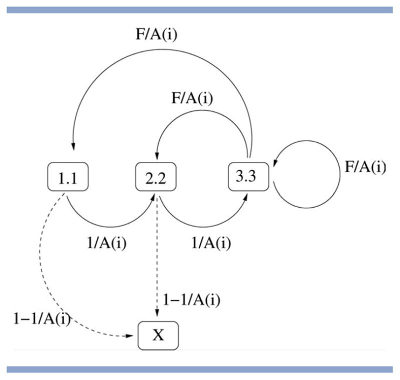
Markov chain describing valid and invalid transitions for M = L = 3 (as used in Stage 4 of Rosetta). A solution string (of N angle triplets) can only be generated by Rosetta if, when read from left to right, it does not lead to absorption in the invalid state X. The probabilities attached to the individual arcs indicate what proportion of A(i) (the number of angle triplets available for position i in the string) will lead to a given transition. Note that state 1.1 is the only possible starting state and that state 3.3 plays a special role in being the only state from which the invalid state cannot be reached directly.

Note that the number of states depends on the size of the fragment L and the move operator M only, whereas transition probabilities are affected by M, L, F, and i. The Markov process always starts in state S = 1, as, by definition of the fragment insertion process, the first angle triplet in the chain is always a starting triplet and any triplet available for this position can be accepted.

For the special case of M = 1, all triplet combinations are accessible (the probability of transition to state X is 0) and the size of the search space equals S☆ above. For M ≥ 2, the portion of the accessible search space for a string of size N corresponds to $1-p_{1.1\to X}^{(N-1)}$, where $p_{1.1\to X}^{(N-1)}$ is the probability of absorption in state X after N − 1 transitions, starting in state 1.1. Given the set of transition matrices P(i) for this Markov chain (the entries of which can be derived directly from the above definitions), $p_{1.1\to X}^{(N-1)}$ is obtained from $P^{(N-1)}={\prod }_{i=2}^{N}P(i)$, which gives the probabilities of moving between any pairs of states after N − 1 transitions. The size of the accessible search space for a string of size N is then given as $(1-p_{1.1\to X}^{(N-1)})\times S^{★}$. An implementation using the GNU multiple precision arithmetic library was used to calculate the size of the accessible space for different choices of L, M, F, and N. The correctness of the model was verified through comparison to the number of unique strings obtained through multiple insertions (only feasible for small L, M, F, and N, results not shown).

Empirical study using a simulation model

A simple simulation model is derived to study the influence of fragment quality on optimal move size, in a controlled manner. The simulation model uses a randomly generated target string consisting of N integers with values in the interval [0,9]. A fragment of length L for each position 1 ≤ a ≤ N is then generated by copying the corresponding section [a,a + L − 1] of the target string. During this process, noise is randomly introduced, that is each position is replaced by a different integer (chosen uniformly at random within [0,9])] with a probability of n. This process is repeated F times, resulting in a fragment library of size F for each position.

This setup is used to obtain random target strings and the corresponding fragment libraries for N = 100, n ∈ {0.0, 0.1, 0.2, 0.3, 0.4, 0.5, 0.6, 0.7, 0.8, 0.9}, L ∈ {1, 3, 6, 9, 12, 15, 18}, and F ∈ {1, 5, 10, 25, 50, 100, 200}. A simple optimiser is then used to minimize the mean squared error (MSE) between the model and the target string. The optimization starts with a random solution (generated uniformly at random). In each iteration, a single insertion (of length M ≤ L) is applied to perturb the current solution. The resulting mutant solution replaces the current solution, if and only if it decreases the MSE. Fragment insertions are implemented analogously to those in Rosetta, with the difference that sampling probabilities are maintained uniformly along the entire string.

We should underline that this model makes a number of simplifying assumptions that reduce its complexity compared to an actual method for protein structure prediction. First, the objective function used is much simpler than the knowledge-based energy functions used in protein structure prediction (in particular, it is decomposable). Second, we use a discrete representation, with a maximum of 10 different values per position (whereas each position in Rosetta corresponds to a torsion angle triplet that exhibits a continuous range of values). Third, we use a very basic model of noise where all fragments are of similar quality (as they are obtained for the same incidence of noise) and the noise of neighboring fragments is uncorrelated. As a direct consequence of our noise model the fragment length L no longer affects the quality of the fragments. In other words, in our simulation model, the role of L is reduced to providing an upper bound on M and determining the size of the search space (whereas L has important implications regarding the quality of the fragment library in a real prediction scenario²¹). Although these assumptions are clearly overly simplistic for the fragment libraries encountered in protein structure prediction, the simulator does allow us to isolate the relationship between fragment quality and optimal move size.

RESULTS

Our key aim in this article is to differentiate between two core parameters of fragment-assembly approaches, which have traditionally been treated as one: the fragment length L and the move size M. Both parameters influence the size and structure of the search space, and we aim to better understand these individual effects, and how the choice of these parameters may impact on the performance of heuristic optimization techniques, as used in state-of-the-art prediction methods. In the following, we first consider the impact of fragment length and move size from a theoretical perspective. We then discuss how these theoretical results relate to observations from empirical analyses using different fragment lengths/moves sizes in Rosetta and in our simulation model.

Size of the search space

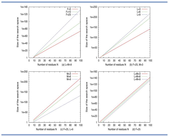
In the section on “Markov chain analysis”, we have derived a Markov chain model to calculate the size of the search space for a given choice of fragment length L, move size M, fragment library size F, and protein length N. Selected results obtained from this theoretical analysis are given in Figure 5. Specifically, panels (a) – (d) show how the size of the search changes as a function of protein length N for a number of different settings of L, F, and M. It is clear that, as protein length increases, the search spaces grows exponentially for all choices of L, M, and F, and that all three of these parameters contribute to determining the asymptotic growth of the search space. For example, Figure 5(a) shows that, for a fixed fragment length L and move size M, the size of the search space increases with increasing F. Similarly, for a fixed fragment library size F and move size M the search space increases more quickly with increasing L [see Fig. 5(b)].

Figure 5.

Asymptotic growth of the search space as a function of protein length N (on a log–linear plot). The search spaces grow exponentially with N, for all choices of L, M, and F. The rate of growth increases with increases in fragment library size F and fragment length L (a and b), but decreases for larger move sizes M (c). If M and L are varied together, the trends observed for L and M cancel out and we observe an identical rate of growth (with different offsets) for all choices of L = M (d). [Color figure can be viewed in the online issue, which is available at wileyonlinelibrary.com.]

Figure 5(c,d) provide the most interesting insight. Figure 5(c) isolates the effect of varying the move size M only. Given a fixed fragment length L and fragment library size F, the rate of growth of the search space increases rapidly with decreasing M. Figure 5(d) shows the effect of varying L and M together using Rosetta's standard restriction of L = M. Our model shows that, for this setting, the effects of L and M [see Fig. 5b,c] counter-balance each other, and that the rate of growth remains identical for different choices of L = M. Large choices of L = M do result in a slightly reduced size of the search space, and this trend is opposite to what would be derived from the naive upper bound S☆, which does not consider the effect of the move size M.

The reduction of the search space through the use of fragments has commonly been cited as one of the reasons behind the success of fragment-assembly techniques (see Ref. 5 and references therein). Our mathematical analysis shows that, for standard methods of fragment-assembly (where L = M), an increase in fragment length results in a net reduction in the size of the search space. However, as the relative change in the size of the search space is surprisingly small, we expect this aspect of fragment length to have little impact regarding the actual performance of the search. Conversely, our analysis shows that independent variation of L or M leads to dramatic differences in the size and the asymptotic growth of the search space. In the following empirical sections, we will establish to what extent performance differences observed for different choices of L and M in Rosetta and our simulation model can be related back to differences in the size of the search space.

Influence of fragment quality

The section on “the dual role of fragments” discussed that, the choice of the move size M can be expected to affect the convergence of heuristic optimisers. These effects arise in addition to the changes in the size of the search space and are not captured by our Markov chain analysis. We thus proceed with an empirical investigation aimed at exploring how optimal move length changes as a function of the difficulty of the optimization task.

We argue that the difficulty of constructing accurate models by fragment assembly increases as the quality of the individual fragments decreases. For example, if all fragments provide exact or very good matches to the corresponding regions of the target protein, they can simply be “strung together” to obtain accurate models. The optimization of an energy function is not strictly necessary in this simplistic setting. Evidently, this situation changes if individual fragments provide poor approximations to the target protein only. We might then still be able to obtain accurate models from the thorough reassembly of the original fragments. However, the identification of these solutions will require the use of an accurate energy function and an effective optimization method that is able to identify the minima of this function. It is at this level that we expect move size to become important, in line with previous research: careful consideration of move size in the optimization literature (see e.g. Refs. ^14–17) suggests that large move sizes may be detrimental for effective optimization.

The results from our simulation model are summarized in Figure 6 and confirm these initial hypotheses. Specifically, Figure 6 summarizes the results for two different settings of fragment library size F and six different settings of L, using the standard restriction that fragment length and move size are identical (i.e., M = L). The figures also include data for selected additional runs, where M and L differ (L = 18 and M = 3). Considering the graphs obtained for different settings with L = M, the results confirm that large moves are only effective for very high quality fragments. For example, the setting of L = M = 18 is optimal for a noise level below 10%. As noise increases in our simulation model, the best performance is observed for increasingly smaller insertions. For example, the setting of L = M = 9 appears to be optimal for noise levels around 20% and a setting of L = M = 6 performs best for noise levels around 30%. For F = 25, the smallest possible move size of M = L = 1 becomes optimal, once a noise level of 70% has been reached. These results suggest that the effectiveness of different move sizes changes with the quality of the fragment set used.

Figure 6.

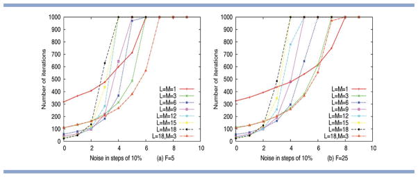
Performance of a simple optimiser using different fragment lengths L and move sizes M as a function of noise for (a) F = 5 and (b) F = 25. We mainly consider settings where L = M (as used in standard Rosetta), but the graph for L = 18, M = 3 is used to illustrate an additional effect of search space size. Performance is assessed using the mean number of iterations required to identify a solution with MSE (≤ 9, over 100 runs). The results demonstrate clearly that optimal move size decreases, as noise levels increase. [Color figure can be viewed in the online issue, which is available at wileyonlinelibrary.com.]

One could argue that differences in the size of the search space may also contribute to the performance differences observed. To reject the null hypothesis that performance differences arise due to changes in the size of the search space only, we therefore consider runs with identical settings of M, but different choices of L. As established previously, the only factor differentiating such runs (in our simulation model) is a change in the size of the search space (see the section on the “empirical study using a simulation model”). In Figure 6, comparison of the results obtained for L = 18, M = 3 and L = M = 3 provides evidence of some performance differences that result directly from changes in the size of the search space. Specifically, Figure 6(a) shows that, for F = 5 and a noise level above 40%, the setting of L = 18, M = 3 outperforms the setting of L = M = 3. It appears that, under these conditions, the optimization directly benefits from the access to the larger parameter space available for the setting L = 18, M = 3. However, Figure 6(b) illustrates that this difference between runs with identical M, but different L, becomes negligible when considering fragment libraries of sufficient size: for F = 25, there is almost no difference between the results obtained for L = 18, M = 3, and L = M = 3. This allows us to conclude that the performance differences observed in Figure 6(b) arise primarily as a consequence of the optimiser's ability to converge, given a specific choice of the move size. However, it is worth pointing out that, in a real prediction scenario, the number of values available per position is less limited (not discrete) than in our simulation model. In Rosetta, performance differences arising from differences in the size of the search space may therefore continue to have some impact on performance for library sizes of F = 25 and beyond.

The effect of move size and fragment length in Rosetta

The experimental results obtained for Rosetta are more complex to interpret than our simulation results above. This is because the software consists of a number of different components whose interplay is crucial in obtaining good prediction performance. The dependencies between these different algorithm components can make it difficult to isolate and analyse the effect of individual changes. For example, the temperature and weight settings in Rosetta are optimized for the current energy terms, and the rigorous evaluation of a new energy term might require changes to these parameters. Similarly, it is likely that optimal temperature or weight settings may vary with fragment size.

In the following subsections, we will aim to illustrate and summarize the key trends observed in Rosetta for the use of different fragment lengths and move sizes. Complete results across the entire test set of 49 proteins are provided in Supporting Information.

RMSD to the native

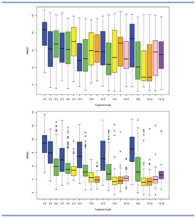
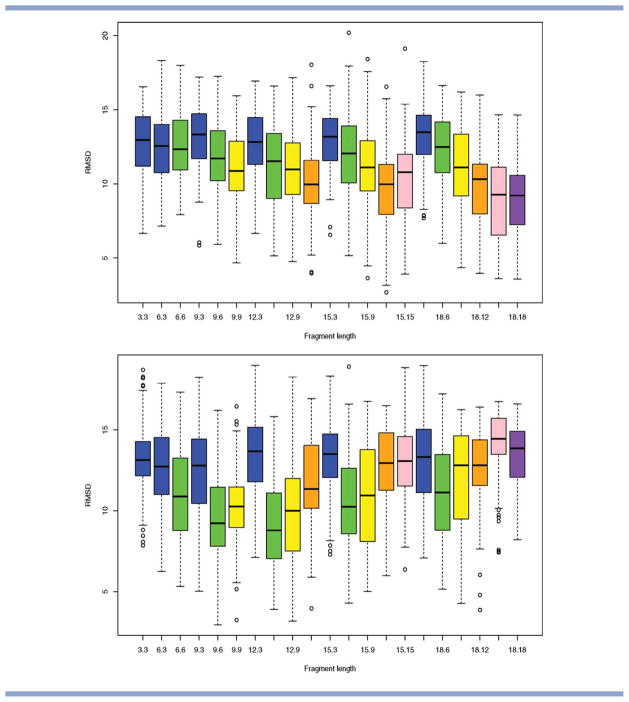
Significant variations in performance are observed for small- to medium-sized beta and alpha-beta proteins. Figures 7 and 8 show the distribution of the RMSD to the native for four such proteins. The figure illustrates that, for these proteins, both fragment length and move size contribute to the performance of the algorithm, albeit in different ways.

Figure 7.

Alpha-beta proteins. Selected results showing the distribution in RMSD to the native obtained as a function of fragment library size and move size (over 100 runs of stage 1 and 2 of Rosetta). Top to bottom: PDB code 1ctf, 1pgx. Results are grouped by fragment length L, and shading is used to identify results that correspond to the same choice of move size M. The distributions are shown in the form of box-and-whisker plots (as implemented in R). The center, top, and bottom of the box correspond to the median, top, and bottom quartile of the distribution, respectively, with the whiskers indicating the minimum and maximum value reached (outliers are indicated by circles). The notation L.M is used to label the results for a fragment length of L and a move length of M and the results appear in lexicographic order. [Color figure can be viewed in the online issue, which is available at wileyonlinelibrary.com.]

Figure 8.

Beta proteins. Selected results showing the distribution in RMSD to the native obtained as a function of fragment library size and move size (over 100 runs of stage 1 and 2 of Rosetta). Top to bottom: PDB code 1tit, 1fna. Results are grouped by fragment length L, and shading is used to identify results that correspond to the same choice of move size M. The distributions are shown in the form of box-and-whisker plots (as implemented in R). The center, top, and bottom of the box correspond to the median, top, and bottom quartile of the distribution, respectively, with the whiskers indicating the minimum and maximum value reached (outliers are indicated by circles). The notation L.M is used to label the results for a fragment length of L and a move length of M and the results appear in lexicographic order. [Color figure can be viewed in the online issue, which is available at wileyonlinelibrary.com.]

First, we consider the difference between runs of Rosetta with the same (fixed) move length (displayed in the same color in Figs. 7 and 8), but where insertions have been derived using a different fragment length. This should allows us to assess the influence of fragment length L: recall that, in Rosetta, both the size of the search space and the identity of the fragments will vary as a function of L. For a number of proteins, we observe distinct differences that arise due to the fragment length L used. For example, for 1ctf, a move size of nine works significantly better in combination with a fragment length of 18 than with a traditional fragment length of nine (compare the yellow boxes in Fig. 7). This is despite the expected increase in the size of the search space for L = 18 [see Fig. 5(b)] and appears to indicate that the fragment library for L = 18 captures additional structural information that is not captured by the library with L = 9.

Overall, the results present no clear evidence favoring a single setting of L, as the “optimal” fragment length appears to vary for different proteins. However, overall, large choices of L (the maximum considered here was L = 18) show a surprisingly robust performance. For the majority of proteins, they perform no worse than shorter fragments when used in combination with a suitable (usually smaller) choice of move size M. One possible reason for this emerges from the analysis of fragment quality (see Fig. 9 and Supporting Information), which indicates that, for the fragment libraries considered, the median of fragment quality tends to remain quite similar for fragment lengths L ∈ [9,18].

Figure 9.

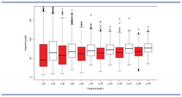
Quality of the fragment libraries. Comparison for PDB code 1fna (dark) and 1tit (white) for F = 25. For each of the fragments, we compute its Euclidean distance (in torsion space) to the corresponding segment of the native structure. The distribution of distances is shown in the form of box-and-whisker plots (as implemented in R). The center, top, and bottom of the box correspond to the median, top, and bottom quartile of the distribution, respectively, with the whiskers indicating the minimum and maximum value reached. [Color figure can be viewed in the online issue, which is available at wileyonlinelibrary.com.]

Second, we consider differences between runs of Rosetta with the same (fixed) fragment length, but different move sizes (grouped together in Figs. 7 and 8). This should provide information about the impact of move size on the optimization. We observe clear differences in RMSD distribution that arise as a result of changes in move size only, and this confirms our initial hypothesis that move size should be considered as a separate parameter. For example, in Figure 8, a fragment length of L = 18 works best in combination with a small move size of M = 6 for PDB code 1tit (a beta protein), whereas it works best in combination with large move sizes for PDB code 1fna (a beta protein of comparable size). Our simulation results from the previous section suggests that such opposite trends may be caused by differences in the quality of the underlying fragment libraries. Analysis of the libraries for these proteins confirms that the fragment library for PDB code 1fna contains a larger proportion of high quality fragments for all fragment lengths considered (see Fig. 9).

For large proteins, Rosetta often fails to generate good quality predictions, and this is likely to be due to problems with the energy function and the sampling protocol used. For these proteins, we see little evidence of differences (in terms of RMSD) between the use of fragments of different length or of different move sizes (see Supporting Information).

Optimization of energy terms

In addition to RMSD to the native, it is instructive to consider also the overall energy scores obtained. Based on our simulation results from the section on the “Influence of fragment quality”, we expect small or medium-sized insertions to lead to the lowest energy scores, as optimization is at its most effective.

For alpha-helical proteins and alpha-beta proteins with predominantly nonlocal strand-pairing (see, e.g., the energy distributions obtained for PDB code 1ail, 1ctf, 1a19 in Supporting Information), the analysis confirms this expectation: large moves appear to prevent convergence and the lowest energy results are usually obtained for small move sizes of M = 3 or M = 6. This is likely to indicate that these move sizes provide the most effective trade-off between escaping local optima in the protein energy landscape and ensuring timely convergence to energy minima.

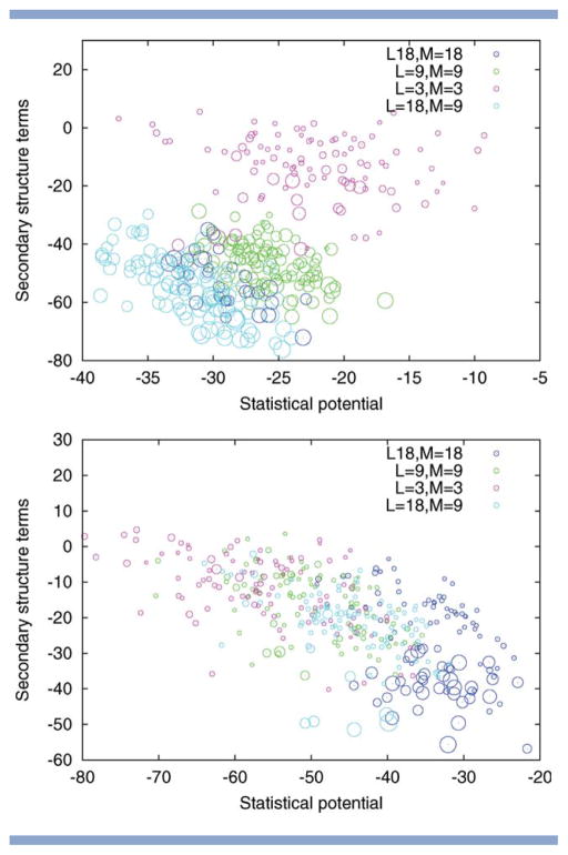
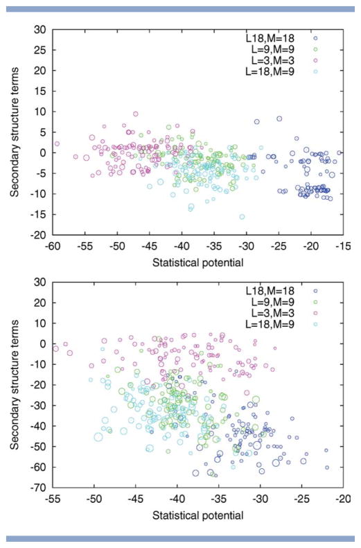
For beta proteins and alpha-beta proteins with predominantly local strand-pairing (see, e.g., energy distributions obtained for PDB code 1acf and 1c8c in Supporting Information) a different result is observed, which appears to be counter-intuitive at first sight: the lowest energy values are obtained for the use of large fragment in combination with medium to large move sets. To understand this phenomenon better, we analyzed individual subscores obtained from summing up the statistical potential, the secondary structure terms, or the compactness terms individually. We observe that the choice of fragment and move size introduces a bias toward specific categories of subscores (see Figs. 10 and 11). In particular, large fragments and moves bias the search toward lower scores in the secondary structure terms. We believe that the reason for this is that large insertions are more likely to span super-secondary structure elements (especially beta-hairpins), resulting in “ready-made” building blocks for the search that, individually, lead to good scores, and are easily retained. On the downside, their retention, and, more generally, the use of large moves, appears to prevent the effective optimization of the statistical potential. There are exceptions to this trend, such as the results for PDB code 1hz6 (see Fig. 10) for which the statistical potential and the secondary structure terms are strongly correlated. However, overall, those decoys that were generated using small moves tend to score better in terms of the statistical potential, which confirms that, as predicted from our simulations, effective optimization/reassembly of fragments is taking place for these small move sizes. The weaker performance of small moves at optimizing the secondary structure terms indicates that the identification of high-scoring secondary structure elements “from scratch” remains one of the current bottlenecks in Rosetta's sampling process.

Figure 10.

Alpha-beta proteins. Two-dimensional visualization of the solutions returned by Rosetta for different choices of fragment length L and move size M. Top to bottom: PDB code 1hz6, 1tig. The size of the circle indicates the quality of the model with larger circles indicating those with a lower RMSD. The position of the circles is determined by the energy subscores corresponding to the statistical potential and the secondary structure terms (both to be minimized). The figure illustrates that the fragment length L and the move size M influence how well these individual subscores are optimized. For PDB code 1tig, variation of L and M results in different trade-offs between the subscores with small moves favoring the statistical potential and large moves biasing the search toward solutions with low secondary structure terms. For PDB code 1hz6, the pattern is different, as the two subscores are correlated, resulting in an overall advantage of runs with large L.

Figure 11.

Beta proteins. Two-dimensional visualization of the solutions returned by Rosetta for different choices of fragment length L and move size M. Top to bottom: PDB code 1bq9, 1c9o. The size of the circle indicates the quality of the model with larger circles indicating those with a lower RMSD. The position of the circles is determined by the energy subscores corresponding to the statistical potential and the secondary structure terms (both to be minimized). The figure illustrates that the fragment length L and the move size M influence how well these individual sub-scores are optimized. Variation of L and M results in different trade-offs between the sub-scores with small moves favoring the statistical potential and large moves biasing the search toward solutions with low secondary structure terms.

Correlation between low energy and RMSD

Regarding the correlation between low energies and low RMSDs, we observe the following trends. For alpha-beta and beta proteins with local strand-pairing, moves derived from large fragments tend to lead to better solutions (see, e.g., PDB code 1ew4 and 1gvp in Supporting Information). This is accompanied by low scores in the secondary structure terms (and overall energies) and is likely due to the direct use of correct super-secondary motifs, as mentioned earlier. In contrast, for beta and alpha-beta proteins with predominantly nonlocal strand-pairing, medium sized moves and fragments tend to fare better in terms of the RMSD (see, e.g., PDB code 1aiu and 1tul in Supporting Information). For these proteins, the effective optimization of the statistical potential appears to translate into an advantage in terms of the RMSD distribution.

For alpha-helical proteins, the lower energies obtained for smaller move sizes do not necessarily correspond to improvements in the RMSD distribution. In contrast, there is a (small) tendency for large move sizes to perform better in terms of the RMSD (see, e.g., RMSD distributions for PDB code 1ail and 1cg5 in Supporting Information) and this also agrees with previous observations in the literature.¹⁸ This is likely to be due to inaccuracies in the energy function. As discussed previously, it is our hypothesis that a small move size facilitates the thorough re-assembly of fragments, which is of course desirable if the energy function is informative. However, it also makes the method more susceptible to deficiencies in the energy function.

CONCLUSION

Fragment insertions are one of the key components of fragment-assembly approaches, which present the state-of-the-art for de novo structure prediction. We have aimed to disentangle and better understand the different ways in which fragment insertions may influence the performance of these techniques. Toward this end, we have defined the separate concepts of fragment length and move size, and have used theoretical and empirical analyses to understand their individual impact.

Recent work has observed that optimal fragment length tends to vary as a function of secondary structure type with larger fragments performing better for alpha-helical proteins, while beta proteins require smaller fragments. It has been argued that this correlates with the relative length of those secondary structure motifs.¹⁸ Our combined results suggest that there are additional reasons behind this phenomenon.

First, we argue that differences in fragment quality will lead to preferences regarding the best move size. The fragments for alpha-helical regions tend to be of significantly higher quality than those for beta sheets³ and this may explain the differences observed in optimal fragment length. As shown in our simulation model, assembly of large fragments can be expected to quickly lead to good solutions if they provide a very good match to the target solution. In the case of alpha-helical proteins, it further appears that the accuracy of the energy function becomes a limiting factor and that, therefore, the lack of convergence in runs that use large move sizes becomes a desirable side-effect. In contrast, it appears that rigorous re-assembly of different fragments and optimization of the energy function is required to obtain accurate models of beta sheet regions and particularly those with nonlocal contacts. In this setting, small- to medium-sized insertions usually display a better performance. This shows that the improved convergence afforded by small move sizes can outweigh the disadvantages incurred by the increase in the search space. In fact, among equally sized moves, we often observe an advantage for moves that derive from larger fragments, which indicates that the models may indeed benefit from the availability of a larger (and different) parameter space.

Second, for proteins that include beta sheets, we observe evidence of direct interactions between fragment length, move size and the optimization of individual energy sub scores. Fragment length and move size strongly bias the search toward particular trade-offs between the energy subscores. Interestingly, the variations observed are more pronounced than those obtained when adjusting the weights in the energy function directly (results not shown). This reveals a strong dependency between these two separate algorithmic components of fragment-assembly methods for protein structure prediction.

Our analysis reveals some overall trends that can be useful in informing the setup of Rosetta. In particular, large fragment lengths with L > 9 show some promise when used in combination with suitable move sizes. For alpha-helical proteins, a choice of a large L (e.g., L = 15 or L = 18) in combination with M = L is usually a robust choice, as this avoids convergence to false local minima of the potential energy landscape. In contrast, the optimal choice of M varies significantly for different alpha-beta and beta proteins. Our advice for such proteins would therefore be to use a large fragment length (e.g., L = 15 or L = 18), but choose different values of M ∈ [6, L] for different runs. The visualization of individual energy scores (as used in Figs. 10 and 11) can be a useful tool in the interpretation of the resulting data, as it helps in identifying those settings for which both the statistical potential and the secondary structure terms are optimized simultaneously. Because of the interactions between fragment/move size and energy subscores, the successful use of different move size may require the adjustment of existing scoring functions. For example, the weight settings typically used in the third and fourth stage of Rosetta's low-resolution protocol heavily bias the search toward secondary structure terms, which (especially for beta proteins) can become problematic in combination with large fragment/move sizes.

As a caveat, we would like to add that our results were obtained for fragment libraries that were generated with homologues excluded. This factor may contribute to the small difference in median fragment quality that we observed for libraries with L ∈ [9,18]. It is possible that, in applications where fragment quality varies strongly as a function of L (e.g., due to the inclusion of homologues), the resulting performance advantages for specific L will dominate the effects discussed in this article.

Suggestions for future developments

Our results are of particular relevance regarding three key areas of future algorithm design in fragment-assembly: (i) the design of improved fragment libraries, (ii) the design of effective variation operators, and (iii) the derivation of weights in knowledge-based energy functions.

Regarding (i) our results indicate that large fragment lengths (in combination with a suitable move size) perform surprisingly well for most proteins. Although further analysis is needed to fully understand this result and to reconciliate it with previous work, our results suggest that a fragment length L of nine or more residues works best for the large majority of proteins considered. Although there is evidence that moves with a size smaller than nine are useful during the optimization, these moves appear to be most effective if they are derived from larger fragments. There may thus be scope to improve existing techniques by maintaining their current move size but moving to larger fragment libraries.

Regarding (ii) our empirical results show that optimal move size varies as a function of fragment quality. Fragment quality is known to vary along the protein chain, and the current, restrictive use of fixed move sizes is therefore bound to be suboptimal. We find that the use of variable moves sizes (deriving from a single fragment length only) shows some promise (results not shown). Furthermore, it may be useful to develop methods that attempt to estimate automatically the quality of a given fragment library, and use such estimates to identify a suitable move size.

Regarding (iii) our results indicate that the move sizes used in fragment-assembly introduce strong biases toward particular energy terms. In the past, this dependency may have contributed to the difficulty of defining general, accurate weight settings, and our improved understanding may help in obtaining more robust parameter settings. Furthermore, move size may be used as an additional means of achieving a consistent optimization of all energy subscores and of driving the search toward the energy trade-offs desired.

References

- 1.Jones D. Predicting novel protein folds by using FRAGFOLD. Proteins. 2001;45(Suppl 5):127–132. doi: 10.1002/prot.1171. [DOI] [PubMed] [Google Scholar]
- 2.Fujitsuka Y, Chikenji G, Takada S. SimFold energy function for de novo protein structure prediction: consensus with Rosetta. Proteins. 2006;62:381–398. doi: 10.1002/prot.20748. [DOI] [PubMed] [Google Scholar]
- 3.Simons KT, Kooperberg C, Huang E, Baker D. Assembly of protein tertiary structures from fragments with similar local sequences using simulated annealing and Bayesian scoring functions. J Mol Biol. 1997;268:209–225. doi: 10.1006/jmbi.1997.0959. [DOI] [PubMed] [Google Scholar]
- 4.Bujnicki MJ. Protein-structure prediction by recombination of fragments. ChemBioChem. 2006;7:19–27. doi: 10.1002/cbic.200500235. [DOI] [PubMed] [Google Scholar]
- 5.Rohl CA, Strauss CE, Misura KM, Baker D. Protein structure prediction using Rosetta. Methods Enzymol. 2004;383:66–93. doi: 10.1016/S0076-6879(04)83004-0. [DOI] [PubMed] [Google Scholar]
- 6.Ben-David M, Noivirt-Brik O, Paz A, Prilusky J, Sussman JL, Levy Y. Assessment of CASP8 structure predictions for template free targets. Proteins. 2009;77(Suppl 9):50–65. doi: 10.1002/prot.22591. [DOI] [PubMed] [Google Scholar]
- 7.Bowman GR, Pande VS. Simulated tempering yields insight into the low-resolution Rosetta scoring functions. Proteins. 2010;74:777–788. doi: 10.1002/prot.22210. [DOI] [PubMed] [Google Scholar]
- 8.Das R. Four Small Puzzles That Rosetta Doesn't Solve. PLoS One. 2011;6:e20044. doi: 10.1371/journal.pone.0020044. [DOI] [PMC free article] [PubMed] [Google Scholar]
- 9.Moult J, Fidelis K, Kryshtafovych A, Rost B, Tramontano A. Critical assessment of methods of protein structure prediction. Proteins. 2009;77(Suppl 9):1–4. doi: 10.1002/prot.22589. [DOI] [PubMed] [Google Scholar]
- 10.Shmygelska A, Levitt M. Generalized ensemble methods for de novo structure prediction. Proc Natl Acad Sci USA. 2009;106:1415–1420. doi: 10.1073/pnas.0812510106. [DOI] [PMC free article] [PubMed] [Google Scholar]
- 11.Bystroff C, Simons KT, Hand KF, Baker D. Local sequence-structure correlations in proteins. Curr Opin Biotechnol. 1996;7:417–421. doi: 10.1016/s0958-1669(96)80117-0. [DOI] [PubMed] [Google Scholar]
- 12.Bowie YU, Eisenberg D. An evolutionary approach to folding small α-helical proteins that uses sequence information and an empirical guiding fitness function. Porc Natl Acad Sci USA. 1994;91:4436–4440. doi: 10.1073/pnas.91.10.4436. [DOI] [PMC free article] [PubMed] [Google Scholar]
- 13.Lee J, Kim SY, Joo K, Kim I, Lee J. Prediction of protein tertiary structure using PROFESY, a novel method based on fragment assembly and conformational space annealing. Proteins. 2004;56:704–714. doi: 10.1002/prot.20150. [DOI] [PubMed] [Google Scholar]
- 14.Hansen N, Ostermeier A. Proceedings of IEEE international conference on evolutionary computation. Nayoya University, Japan: IEEE Press; 1996. Adapting arbitrary normal mutation distributions in evolution strategies: the covariance matrix adaptation; pp. 312–317. [Google Scholar]
- 15.Igel C, Kreutz M. Operator adaptation in evolutionary computation and its application to structure optimization of neural networks. Neurocomputing. 2003;55:347–362. [Google Scholar]
- 16.Lin S, Kernighan BW. An effective heuristic algorithm for the traveling-salesman problem. Oper Res. 1973;21:498–516. [Google Scholar]
- 17.Mladenovi N, Hansen P. Variable neighborhood search. Comput Oper Res. 1997;24:1097–1100. [Google Scholar]
- 18.Raman S, Vernon R, Thompson J, Tyka M, Sadreyev R, Pei J, Kim D, Kellogg E, DiMaio F, Lange O, Kinch L, Sheffler W, Kim BH, Das R, Grishin NV, Baker D. Structure prediction for CASP8 with all-atom refinement using Rosetta. Proteins. 2009;77(Suppl 9):89–99. doi: 10.1002/prot.22540. [DOI] [PMC free article] [PubMed] [Google Scholar]
- 19.Gront D, Kulp DW, Vernon RM, Strauss CEM, Baker D. Generalized fragment picking in Rosetta: design, protocols and applications, 2011. PLoS ONE. 6(8):e23294. doi: 10.1371/journal.pone.0023294. [DOI] [PMC free article] [PubMed] [Google Scholar]
- 20.Metropolis N, Rosenbluth AW, Rosenbluth MN, Teller AH, Teller E. Equation of state calculations by fast computing machines. J Chem Phys. 1953;21:1087–1092. [Google Scholar]
- 21.Bystroff C, Baker D. Prediction of local structure in proteins using a library of sequence-structure motifs. J Mol Biol. 1998;281:565–757. doi: 10.1006/jmbi.1998.1943. [DOI] [PubMed] [Google Scholar]
- 22.Brunette TJ, Brock O. Guiding conformation space search with an all-Atom energy potential. Proteins. 2009;73:958–972. doi: 10.1002/prot.22123. [DOI] [PMC free article] [PubMed] [Google Scholar]
Associated Data
This section collects any data citations, data availability statements, or supplementary materials included in this article.