Detection and Integration of Genotyping Errors in Statistical Genetics

Abstract

Detection of genotyping errors and integration of such errors in statistical analysis are relatively neglected topics, given their importance in gene mapping. A few inopportunely placed errors, if ignored, can tremendously affect evidence for linkage. The present study takes a fresh look at the calculation of pedigree likelihoods in the presence of genotyping error. To accommodate genotyping error, we present extensions to the Lander-Green-Kruglyak deterministic algorithm for small pedigrees and to the Markov-chain Monte Carlo stochastic algorithm for large pedigrees. These extensions can accommodate a variety of error models and refrain from simplifying assumptions, such as allowing, at most, one error per pedigree. In principle, almost any statistical genetic analysis can be performed taking errors into account, without actually correcting or deleting suspect genotypes. Three examples illustrate the possibilities. These examples make use of the full pedigree data, multiple linked markers, and a prior error model. The first example is the estimation of genotyping error rates from pedigree data. The second—and currently most useful—example is the computation of posterior mistyping probabilities. These probabilities cover both Mendelian-consistent and Mendelian-inconsistent errors. The third example is the selection of the true pedigree structure connecting a group of people from among several competing pedigree structures. Paternity testing and twin zygosity testing are typical applications.

Introduction

All large genotype data sets have errors. These mistypings can be due to human oversights, to shortcomings in genotype scoring software, or simply to biochemical anomalies. Unfortunately, error rates are likely to increase as laboratories turn to single-nucleotide polymorphisms (SNPs) and rush to implement high-throughput methods. Several authors have shown that even a small (1%–2%) error rate can have an enormous impact on linkage results (Buetow 1991; Goldstein et al. 1997; Douglas et al. 2000; Abecasis et al. 2001). However, it is rare for linkage studies to catch all errors and even rarer for statistical geneticists to explicitly account for errors in analysis.

As a typical example of the confusion caused by genotyping errors, in May 2001 The New York Times published an article (Angier 2001) describing how a startling new paradigm for chimpanzee mating behavior, proposed in 1997 and widely accepted in primatology circles, had recently been overturned. The original research (Gagneux et al. 1997) concluded that female chimpanzees frequently engaged in “furtive” mating outside their social group and that more than half the infants born in the group were the issue of extragroup liaisons. This research was widely reported by the mainstream press and taken up in the public imagination (Angier 1997). The conclusions were reversed in a later study by another group (Constable et al. 2001). Dr. Pascal Gagneux, one of the authors of the original study, was forced to confess in the national press: “I unfortunately have to agree with them that there seem to be serious problems with my genotyping results. I was not being conservative enough in scoring the genotypes. This is obviously extremely embarrassing to me” (Angier 2001, p. F3).

We can sympathize with Dr. Gagneux and his colleagues, since the problem of identifying genotyping errors is a difficult one. In a large study, it is nearly impossible to identify all errors manually. Statistical geneticists have devised a variety of automatic screening methods to spot marker errors and their probable sources (Lincoln and Lander 1992; Brzustowicz et al. 1993; Ott 1993; Ehm et al. 1996; Stringham and Boehnke 1996; O’Connell and Weeks 1998, 1999; Douglas et al. 2000). Unfortunately, none of these methods are complete or general enough to catch all errors. This is a subtler problem than one might at first assume. There are two types of errors: those inconsistent with Mendelian inheritance—commonly known as “Mendelian errors”—and those consistent with Mendelian inheritance. Many genotyping laboratories are content to detect and delete only Mendelian errors. Although the Mendelian-consistent errors are much harder to detect, they still can have a profound influence on the validity of statistical analysis. For example, many of the observed close double recombinants that lead to unexplained map expansions in genome scans are Mendelian consistent. Such errors usually constitute ⩾25% of all mistypings in fully typed nuclear family data (Douglas et al. 2002 [in this issue]). Even overt Mendelian errors are contextual and can often be attributed to more than one source within a pedigree. The difficulty of detecting genotyping error can only intensify with the increased use of SNPs, since a greater proportion of typing errors with a biallelic marker is Mendelian consistent (Gordon et al. 1999a; Gordon and Ott 2001).

Although often ignored in practice, the impact of genotyping errors on statistical results has been recognized since the 1930s (Smith 1937). Several recent articles have described these effects in some detail (Daw et al. 1998; Gordon et al. 1999a, 1999b; Göring and Terwilliger 2000a; Akey et al. 2001). Mistyping affects two areas of genetic analysis: (1) the accuracy of the marker map (Terwilliger et al. 1990; Lunetta et al. 1995; Goldstein et al. 1997) and (2) the localization of traits (Terwilliger et al. 1990; Buetow 1991; Heath 1998; Abecasis et al. 2001). Several methods of compensating for these errors have been proposed (Ott 1977; Brzustowicz et al. 1993; Göring and Terwilliger 2000b, 2000c, 2000d; Gordon and Ott 2001), but such methods are not in common use. In the present study, we propose a straightforward solution that integrates realistic error models with likelihood-based pedigree analysis.

Likelihood algorithms are the “engines” for much of modern statistical genetics. If these algorithms can be extended to accommodate mistyping, then statistical analysis can be performed without the need to detect and then manually correct or delete genotyping errors. Gordon et al. (2001) discuss a method for doing exactly this, in the limited context of the transmission/disequilibrium test on SNP data. Clearly, some strategy of this kind will be necessary for genetic analysis to keep pace with advances in high-throughput genotyping. Currently, a single technician can generate as many as 10,000 genotypes per day. Here we present extensions to two widely used likelihood algorithms, namely the Lander-Green-Kruglyak deterministic algorithm, designed for small pedigrees (Lander and Green 1987; Kruglyak et al. 1996; Kruglyak and Lander 1998), and the Markov-chain Monte Carlo (MCMC) stochastic algorithm, designed for large pedigrees (Lange and Matthysse 1989; Lange and Sobel 1991; Guo and Thompson 1992; Sobel and Lange 1993; Thompson 1994, 1996). Almost any pedigree can be analyzed by one of these two techniques.

In the first section below (Error Models), we discuss the error models required by the extended likelihood algorithms. Genotyping error is random—not in the sense that it is uniformly distributed, but in the sense that it is uncertain. One of the challenges of statistical genetics is to model how errors occur. Once a model is constructed, it can be used in likelihood analysis to relate observed genotypes to hidden true genotypes. In the past, barriers of computational complexity have limited the application and generality of these error models. One method of avoiding some of the complications has been to allow, at most, one error per pedigree (Ehm et al. 1996). In the present article, we argue that such compromises are unnecessary and that implementation of realistic error models is feasible. After discussing error models, we take up the algorithmic adjustments necessary to incorporate these models into pedigree likelihood calculations.

Most of the remainder of the article considers three specific examples where error models can be integrated in statistical analysis. The first example involves estimation of mistyping rates from genotype data. It is possible to estimate either global error rates or locus-specific error rates by using data on all loci simultaneously. Estimated error rates are good measures of quality and can provide useful feedback to improve the genotyping process.

Our second—and currently most important—example is the detection of genotyping errors. We have alluded to the difficulty of this problem and the many past efforts in the automation of mistyping detection. Our approach is to employ an a priori error model to calculate, at each observed genotype, a posterior probability of mistyping. Although this natural and powerful method has certainly been suggested previously, the computational baggage it carries has restricted previous applications to simple error models, specific pedigree structures, or single-locus computations (Ehm et al. 1996; Stringham and Boehnke 1996; Douglas et al. 2000, 2002 [in this issue]). Recently, for example, Douglas et al. (2000) implemented this strategy for sibling data, in their program SIBMED. We show that it is now feasible to compute posterior mistyping probabilities for multilocus data on general pedigrees while using general error models.

Our third and final example deals with the problem of choosing among competing pedigree structures connecting a group of people. Several authors address this problem for pairs of relatives (Thompson 1975, 1986; Boehnke and Cox 1997; Ehm and Wagner 1998; McPeak and Sun 2000). Some authors even allow for genotyping errors in their pedigree error analyses (Lathrop et al. 1983; Broman and Weber 1998; Kumm et al. 1999; Sieberts et al. 2001). To our knowledge, however, no current implementation successfully handles general pedigrees and general error models. Our Bayesian approach does and is worth discussing for that reason.

These three sample analyses have been implemented in the program MENDEL, version 4 (Lange et al. 1988), using the Lander-Green-Kruglyak algorithm. The estimation of posterior mistyping probabilities has been implemented in the program SimWalk2, version 2.82 (Sobel and Lange 1996), using the MCMC algorithm.

Error Models

One of the difficulties in dealing with genotyping error is that previously simple codominant markers become complex. Each observed genotype must now be treated as a phenotype, since any underlying genotype is, in principle, consistent with any observed genotype. In the shift from codominant genotypes to less definite phenotypes, pedigree likelihood computations need to sum—or, in the case of MCMC, to sample from—all genotypes rather than a limited range of genotypes. In addition, a penetrance-weighting factor must be incorporated in the likelihood as the computations visit each of the possible underlying genotypes. This penetrance factor is just the conditional probability Pr(observedgenotype|underlyinggenotype). If one ignores mistyping, each marker penetrance term is either one or zero, depending on whether a possible underlying genotype equals an observed genotype or not. When mistyping is taken into account, penetrances lie somewhere between these extreme values. The penetrance function embodies an error model for purposes of likelihood calculation.

In discussing genotyping errors, several authors have posited a uniform distribution of errors over the available genotypes at a single locus (Lincoln and Lander 1992; Ott 1993; Ehm et al. 1996). We can accordingly define the penetrance φ(g₁/g₂|t₁/t₂) of an observed marker genotype g₁/g₂, given a possible underlying marker genotype t₁/t₂, as

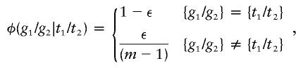where ε is the error rate per genotype, both genotypes are unordered, and there are m genotypes in all. Another simple model distributes errors over alternative genotypes in proportion to their population frequencies. In other words,

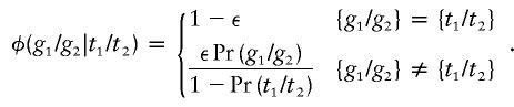Both of these models are biologically unrealistic. Perhaps more importantly, both models involve the kind of fuzzy phenotypes that lead to long computation times. One can circumvent the computational bottlenecks by lumping all alleles not seen in a pedigree into a single alternative super allele. The small inaccuracies this action creates in estimating posterior probabilities under the uniform model are compensated for by huge savings in computation times. When errors are made in proportion to genotype frequencies, posterior probabilities are unaffected by allele lumping.

As an alternative to these straightforward error models, one can develop empirical models. In our experience of checking more than a million genotypes, errors are not uniformly distributed, and certain types of error predominate. For example, when automated software or trained technicians genotype by scoring bands on a gel, the most common error is false homozygosity. An error occurs in this case when an allele amplifies insufficiently or a band falls outside a prescribed range. A second type of error, common in heterozygotes, involves misreading an allele. For example, one might incorrectly call one of the neighboring “stutter” bands rather than the true peak on a gel. Although one may independently misread both alleles of a genotype, correlated errors that cause both alleles to be mistyped are more frequent, even in homozygotes. Jointly misreading both alleles is our third type of error. For example, in a “gel-shift,” the sample DNA does not pass through the gel at the same rate as the DNA standards; this causes both alleles to be misinterpreted. A fourth type of error involves adding an allele because of a false band—for example, misinterpreting a stutter band as a second allele. For slab-based gels, this kind of false heterozygosity also happens because of spillover from adjacent lanes or spectral bleed-through of a dye to another wavelength. Capillary-based gels are not subject to spillover, but bleed-through can still occur. Finally, there are pre-gel errors, such as sample swap or pipetting mistakes, that may have any effect. The pre-gel category provides a lower bound on the error rates in the specific classification of errors discussed below.

The five types of errors—missing an allele, misreading an allele, jointly misreading both alleles, adding an allele, and pre-gel errors—have independent sources and, in our experience, different rates, which we denote by ε₁ through ε₅, respectively. For a locus with n alleles, the penetrance φ(g₁/g₂|t₁/t₂) can be approximated by the simple algorithm shown in figure 1. If n<4, then several of the penetrances in figure 1 revert to 0. For example, if n=3, then the last penetrance term listed in figure 1 becomes 0, since one cannot have two completely distinct heterozygous genotypes with only three alleles. Accordingly, the second “no errors” penetrance reduces to 1-(ε₁+ε₂+ε₅). In the various penetrance expressions with a denominator, the denominator represents the number of possible observed genotypes in the corresponding class.

Figure 1.

Empirical penetrance model

All of these error models are simple to implement in analysis and provide users with several options. The optimal values for the error rates will vary with the genotyping hardware and software, the marker loci, and the expertise of the responsible technicians. Our default error rate for the uniform model is ε=0.025. For the empirical model, our default rates are ε₁=0.0125, ε₂=0.0075, ε₃=0.0050, ε₄=0.0100, and ε₅=0.0025. These translate into an overall error rate of ε₃+ε₄+ε₅=0.0175 when the true genotype is homozygous and to ε₁+ε₂+ε₃+ε₅=0.0275 when it is heterozygous. The fact that true heterozygotes have a higher rate of mistyping seems intuitive, given the more numerous sources of error. An error model based only on the homozygote/heterozygote dichotomy would be another option. For inexperienced genotypers or an unoptimized marker set, all these rates should be scaled up, perhaps by a factor of two or three. As discussed below, one can also estimate error rates given an error model and fairly small pedigrees. These estimates can provide a useful reality check on the error model.

Deterministic Algorithms on Small Pedigrees

Our deterministic descent-graph method of analysis relies on an extension of the Lander-Green-Kruglyak algorithm for likelihood calculation. This extension allows the algorithm to handle noncodominant loci, such as marker loci with genotyping errors. Although the program GENEHUNTER, implementing the Lander-Green-Kruglyak algorithm, does have the capacity to handle a specific type of noncodominant locus, namely, recessive traits in homozygosity mapping, the underlying penetrance algorithms are poorly documented (Lander and Green 1987; Kruglyak et al. 1995, 1996; Kruglyak and Lander 1998). Here we discuss an algorithm that can accommodate arbitrary penetrance functions at either trait or marker loci. This innovation in likelihood evaluation makes the descent-graph method fully equivalent to the Elston-Stewart method (Elston and Stewart 1971) under the conditions of (a) Hardy-Weinberg and linkage equilibrium; (b) Haldane’s Poisson model of recombination—namely, no interference; and (c) phenotypically noninteracting loci—namely, no epistasis. Such equivalence facilitates closer integration of the two methods and selection of the faster method for any given pedigree.

As part of its overall hidden Markov-chain strategy, the deterministic descent-graph method proceeds sequentially from one locus to the next. Here we ignore how the method accounts for transitions between loci, and we focus on how penetrances and priors are incorporated at a single locus, given assumptions a, b, and c above. Readers interested in other details of the algorithm can consult the original articles cited above. Descent graphs determine gene flow patterns within a pedigree but do not specify which alleles flow along a given path. (The terminology of descent graphs used here was introduced by Sobel and Lange [1996] and is covered in detail by Lange [1997]. Other authors prefer the term “inheritance vector.”) The crux of the matter is to compute the likelihood of the phenotypes at the locus, conditional on a given descent graph. Figure 2a depicts a typical descent graph and results of partial typing at the locus. Figure 2b shows a second graph constructed by connecting some of the founder genes. Two founder genes are connected by an edge in figure 2b if they flow through some common typed person. For example, founder genes F and H are connected because they both pass to the grandchild with phenotype 2/4.

Figure 2.

Construction of a founder gene graph. a, Descent graph. b, Connected founder genes.

In this example with codominant alleles and no typing error, the conditional likelihood of the pedigree splits into three independent factors corresponding to the three connected components of the graph shown in figure 2b. Consider the component containing founder genes A, C, and E. If we assign allele g_A to founder gene A, allele g_C to founder gene C, and allele g_E to founder gene E, then the conditional likelihood associated with the component is the product p_gAp_gCp_gE of the corresponding population allele frequencies, provided that the assigned alleles are compatible with all of the individuals through whom they pass. In generalizing this representative computation to more complicated models involving noncodominant loci, we must multiply the prior p_gAp_gCp_gE by the penetrances of all relevant people and then sum over all possible assignments of the allele vector (g_A,g_C,g_E).

If there are n alleles at the locus under consideration, then there are n³ possible assignments to the allele vector (g_A,g_C,g_E). For the simple either/or penetrance functions encountered with perfectly typed markers, many values for the allele vectors can be eliminated as incompatible with observed phenotypes. For instance, with codominant alleles, the only compatible assignments here are (g_A,g_C,g_E)=(1,2,1) and (g_A,g_C,g_E)=(2,1,2). This observation tremendously simplifies matters and makes it clear that quick elimination of most incompatible allele vectors is key to fast computation, as has been highlighted elsewhere (Kruglyak et al. 1996; Sobel and Lange 1996).

To extend these arguments to more-complicated penetrance models, we now suggest a backtracking scheme for systematic examination of allele vectors and quick elimination of incompatible vectors (Nijenhuis and Wilf 1978). In backtracking, one attempts to grow a compatible allele vector from partial vectors that are compatible. In the codominant case of our example, we start with the assignment (g_A)=(1), which is consistent with the phenotypes in the pedigree; grow it to (g_A,g_C)=(1,1), which is inconsistent; discard all vectors beginning with (g_A,g_C)=(1,1); move on to (g_A,g_C)=(1,2), which is consistent; grow this to (g_A,g_C,g_E)=(1,2,1), which is consistent; move on to (g_A,g_C,g_E)=(1,2,2), (g_A,g_C,g_E)=(1,2,3), and (g_A,g_C,g_E)=(1,2,4), which are inconsistent; backtrack to (g_A,g_C)=(1,3), which is inconsistent; and so forth. The primary virtue of backtracking is that it eliminates large numbers of incompatible vectors without actually visiting each of them.

For loci with recessive alleles, we can also perform backtracking by repeatedly checking for consistency among those people whose genotypes are impacted by a partial allele vector. Again, many of these partial vectors can be rejected. In the extreme situation presented by error models where every genotype is consistent with every phenotype, the backtracking method has little to offer beyond a systematic way of enumerating allele vectors. The computational complexity of penetrance evaluation in the extreme case is n^2f per descent graph at a locus with n alleles in a pedigree with f founders. When symmetries are counted, the number of descent graphs per locus is 2^2c-f when the pedigree contains c children. When the Walsh transform is used (Keener 1988), it takes on the order of (2c-f)2^2c-f arithmetic operations for the Lander-Green-Kruglyak algorithm to proceed from one locus to the next (Kruglyak and Lander 1998). Thus, the overall computational complexity for l loci is on the order of

This figure can balloon out of control if n is large; however, when the allele-lumping strategy discussed above is used, n stays small in small pedigrees, and the computation load remains reasonable.

Stochastic Algorithms on Large Pedigrees

As the size of a pedigree increases, enumerating all descent graphs becomes computationally impossible. For large pedigrees, we must turn to stochastic methods. In the past, we and other researchers have developed two types of stochastic algorithms for pedigree analysis. One of these relies on descent graphs; the other relies on descent states, which are simply descent graphs with all founder alleles specified. Descent graphs are preferable in the sense that there are fewer of them and that they normally present less rigidity in Markov-chain sampling. However, descent graphs require the kind of complicated enumeration of allele vectors discussed above. Descent states avoid this complication, so we have elected to use them for stochastic computation of pedigree likelihoods in the presence of genotyping errors. The normally poor communication between descent states is mitigated by the incorporation of genotyping error, since this allows any genotype at any locus.

Regardless of the specific error model used, all posterior error probabilities reduce to simple conditional probabilities. Let M denote the collection of observed genotypes in a pedigree and A_ij the event that the true genotype and observed genotype match at locus j of individual i. The posterior probability of no error at this locus and individual is just the conditional probability Pr(M∩A_ij|M). Given the correct penetrance function implementing the genotyping error model in the Markov chain, one can approximate this conditional probability stochastically as the proportion of time in the Markov-chain simulation that the sampled and observed genotypes match. In addition to obviating the need for a time-consuming backtrack scheme, the use of descent states, rather than descent graphs, simplifies the determination of when theoretical genotypes match observed genotypes.

When one proceeds deterministically on small pedigrees, it is easiest to evaluate Pr(M∩A_ij) and Pr(M) separately and divide. A trivial adjustment of the genotyping penetrance function accounts for the difference between these probabilities. As previously mentioned, it helps in the deterministic computations to reduce the set of possible alleles at each locus to those actually seen in the pedigree. This is also helpful in the stochastic computation, since reducing the number of alleles reduces the descent-state space and thus permits more-thorough sampling in a shorter time. In either case, allele lumping may change posterior probabilities slightly, but the decrease in computing time easily justifies the shortcut.

Descent-state MCMC methods allow analysis of almost any realistic pedigree. Of course, the usual caveats apply. On small pedigrees, results from the deterministic method are preferred, even though our tests show excellent agreement between the two methods. For truly large pedigrees, lengthy—and, perhaps, repeated—MCMC runs are recommended.

Example 1: Estimation of Error Rates

Genotyping methods vary from laboratory to laboratory around the world, and accuracy can differ even within a laboratory, from technician to technician. Clearly, it is important to judge the quality of data sets before merging them. Any method for gauging quality has the collateral benefit of allowing a laboratory to improve and refine its typing protocols. Many laboratories use the proportion of Mendelian inconsistencies in their data as their primary measure of genotyping quality. Unfortunately, this fails to account for the errors that are Mendelian consistent—errors that are likely to be particularly abundant in biallelic markers. Duplicate typing is a good method of estimating error rates, even though it captures consistency rather than accuracy. The expense of duplicate typing argues in favor of statistical procedures for checking error rates.

Here we discuss an example of maximum-likelihood estimation of error rates under the uniform error model. The data were taken from a genome scan of seven nuclear families with ⩽10 members each. Genotypes were generated on the ABI PRISM 377 DNA Sequencer, using the ABI PRISM Linkage Mapping Set–MD10 markers. In our example, we started with 28 markers on chromosome 1, 17 markers on chromosome 9, and 5 markers on chromosome 21, with an average distance of ∼10 cM between adjacent markers. Maximum-likelihood estimation of the error rates was conducted on three versions of the genotypes: (a) the gels were run through the ABI PRISM Genotyper 2.5 software, and the genotypes were taken directly as assigned by the program, with no manual scoring; (b) the gels that were first scored by Genotyper software were then manually scored by a technician with >2 years of experience reading ABI gels; and (c) the manually scored genotype data were cleaned using a variety of quality-control checks developed in our laboratory (Papp et al. 2000).

Some of the quality-control checks, such as thresholds for acceptable allele sizes, intensity, and morphology, are applied to single genotypes. Other checks use characteristics such as homozygosity, allele frequencies, and overall success rates that are calculated across entire data sets. Once these preliminary checks are done, data are grouped in a variety of ways—for example, by study, by gel, or by date—and examined for anomalous patterns and outliers. All of these checks flag questionable genotypes, which are then rechecked by inspecting the raw data from the gel image. All genotyping, including the quality-control checking, was done blind to the pedigree structure, and, hence, without checking for Mendelian errors. Pedigree information was only incorporated at the time of error-rate estimation. The number of markers that were considered to be of acceptable quality for typing decreased when moving from the automated software to the manual scoring to the quality-control stages.

Table 1 displays the estimated error rates for the three chromosomes noted above. These results are representative of the different patterns we have seen. The estimates in table 1 track the decline in the overall mistyping rate as the data proceed through the different steps of the genotyping process. Obvious differences in the results from these three chromosomes reflect the characteristics of different markers. Chromosome 1 shows a steady decline in error rate from automated genotyping to manual scoring to quality-control stages. This is by far the most common pattern we have seen. Chromosome 9 markers were scored quite successfully by the genotyping technician on the manual pass, leaving little room for further improvement by the quality-control procedures. Chromosome 21 shows a high overall error rate that declines only slightly through the quality-control process. Further investigation found that, at the quality-control stage, the locus-specific error rate was 0.2860 for one of the markers on chromosome 21. Clearly, this marker was not genotyping well and should be either reoptimized or replaced. After deleting this bad marker, the estimated global error rate fell to 0.0001 (with 64 observed genotypes) at the quality-control stage.

Table 1.

Estimated Error Rates on Three Chromosomes for Genotypes Generated by Three Different Procedures, All without Access to Pedigree Structure^[Note]

	Error Rate (No. of ObservedGenotypes) for Scoring Method
Chromosome	Genotypera	Manual Scoring	Quality Controlb
1	.0436 (821)	.0209 (744)	.0001 (601)
9	.0555 (511)	.0004 (399)	.0001 (211)
21	.1272 (151)	.0831 (103)	.0715 (90)

Note.— A lower bound of .0001 on error rates was enforced during maximum-likelihood estimation.

^aData scored by Genotyper software, with no manual scoring.

^bData cleaned by our quality-control procedures.

It may seem from the results in table 1 that by applying rigorous error checking, one is discarding large amounts of data that represent weeks of work in the laboratory. However, clinging to questionable data is penny-wise but pound-foolish. At the worst, rejecting data may be cause for repeating some runs. This extra effort must be balanced against the unattractive alternatives of having linkage evidence masked by genotyping errors or declaring linkage where none exists.

False positives can be nearly as detrimental as false negatives. A colleague of ours obtained a LOD score of 2.98 linking a trait to a single marker, although surrounding markers all gave low LOD scores. The data were checked for Mendelian errors prior to statistical analysis but were not subjected to the quality-control process mentioned above. When we computed posterior error probabilities, as discussed in the next section, the results sent her back to the gels to re-evaluate their scoring. She then verified and corrected a series of genotyping errors on a single gel and repeated her linkage analysis. The maximum LOD score at the suggested marker went down to 0.55. If she had not run the mistyping analysis, she would have spent a great deal of time and money in fine mapping a region with no real evidence for linkage.

Finally, it is worth noting that the computational complexity of the deterministic likelihood algorithm limits error-rate estimation to fairly small pedigrees. As a rough guide, the bound 2c-f⩽14 should hold, where c is the number of children (nonfounders) and f is the number of founders in the pedigree.

Example 2: Posterior Probability of Mistyping

Checking for Mendelian errors in genotype data is currently standard practice, since these errors must be removed before almost any statistical analysis package will run. Some researchers proceed a step further and use haplotyping programs, including our own, to detect apparent double recombinants in small regions and to infer the locations of the responsible Mendelian-consistent mistypings. Although the application of haplotyping for this purpose is preferable to ignoring these errors, it is far from perfect. For one thing, current programs provide a single haplotype configuration when, in fact, there may be many equally likely or only slightly less likely alternative configurations consistent with the data.

The posterior-probability method gives more-definitive predictions by, in essence, considering the distribution of all possible haplotypes. Computation of posterior probabilities depends on the usual parameters of pedigree likelihoods: allele frequencies, marker map distances, and a penetrance function, in this case determined by an error model. Predictions are reasonably robust to small perturbations in these quantitative parameters but can show sensitivity to gross errors in pedigree structure or the order of marker loci. As discussed in the next section, such sensitivity can be useful in detecting nongenotyping errors.

To illustrate the posterior-probability method, we use some of the same data featured in Example 1. Tables 2, 3, and 4 give output from a single nuclear family with data from chromosome 9. In this case, genotypes are taken directly from the automated genotype-calling software. The individuals labeled 24–30 are the children of the nuclear family. There were 17 loci included in our analysis, with ⩽13 alleles per locus. These tables show only the output for five of the last six loci, an interesting and representative subset.

Table 2.

Part of the Output from a Mistyping Analysis Using MENDEL, Version 4^[Note]

Locus and Individual	Error Probabilitya
D9S1677:
Anyone	.00486
Father	.00000
Mother	.00000
24	.00003
25	.00304
26	.00094
27	.00003
28	.00003
29	.00031
30	.00049
D9S1776:
Anyone	1.00000
Father	.02751
Mother	.00001
24	.00002
25	.97262
26	.00037
27	.00002
28	.00016
30	.00073
D9S1682:
Anyone	.73744
Father	.62274
24	.00173
25	.01259
26	.00647
27	.00174
28	.00223
30	.09940
D9S290:
Anyone	.61366
Father	.00026
Mother	.56709
24	.00008
25	.00056
26	.04476
27	.00008
28	.00254
30	.00034
D9S1826:
Anyone	1.00000
Father	.00015
Mother	.00000
24	.01475
25	.00067
26	.00044
27	.00044
28	.00133
29	.99995
30	.00037

Note.— For each observed genotype, a posterior probability of mistyping is calculated via the Lander-Green-Kruglyak algorithm, with the penetrance function at these loci based on a uniform error model with error rate .025.

^aGenotype mistyping probabilities >.25 are underlined.

Table 3.

Part of the Output from a Mistyping Analysis Using SimWalk2, Version 2.82 (Uniform Error Model)^[Note]

		Probability of Mistyping ata
Locus andIndividual	ObservedGenotypeat Allele 1/Allele 2	Allele1	Allele2	BothAlleles	EitherAllele
D9S1677:
Father	01/05	.000	.000	.000	.000
Mother	07/09	.000	.000	.000	.000
24	01/07	.000	.000	.000	.000
25	05/09	.001	.001	.001	.001
26	01/09	.001	.001	.001	.001
27	01/07	.000	.000	.000	.000
28	01/07	.000	.000	.000	.000
29	01/09	.001	.000	.000	.001
30	05/07	.000	.000	.000	.000
D9S1776:
Father	04/04	.012	…	.000	.012
Mother	05/06	.000	.000	.000	.000
24	04/06	.000	.000	.000	.000
25	05/06	.233	.756	.000	.989
26	04/05	.000	.002	.000	.002
27	04/06	.000	.000	.000	.000
28	04/06	.000	.001	.000	.001
30	04/06	.000	.001	.000	.001
D9S1682:
Father	01/02	.394	.287	.000	.681
24	01/02	.000	.000	.000	.000
25	01/02	.003	.003	.000	.006
26	01/02	.003	.002	.000	.005
27	01/02	.000	.000	.000	.000
28	01/02	.001	.003	.000	.004
30	01/02	.042	.049	.000	.091
D9S290:
Father	02/06	.000	.000	.000	.000
Mother	04/06	.605	.000	.000	.605
24	06/06	.000	…	.000	.000
25	02/06	.000	.000	.000	.000
26	02/06	.006	.037	.000	.043
27	06/06	.000	…	.000	.000
28	06/06	.005	…	.000	.005
30	02/06	.000	.000	.000	.000
D9S1826:
Father	04/04	.000	…	.000	.000
Mother	02/04	.000	.000	.000	.000
24	02/04	.008	.000	.000	.008
25	04/04	.000	…	.000	.000
26	02/04	.000	.000	.000	.000
27	04/04	.000	…	.000	.000
28	02/04	.001	.000	.000	.001
29	03/04	1.000	.000	.000	1.000
30	04/04	.000	…	.000	.000

Note.— For each observed genotype, a posterior probability of mistyping is calculated via an MCMC algorithm, with the penetrance function at these loci based on a uniform error model with error rate .025.

^aGenotype mistyping probabilities >.25 are underlined.

Table 4.

Part of the Output from a Mistyping Analysis Using SimWalk2, Version 2.82 (Empirical Error Model)^[Note]

		Probability of Mistyping ata
Locus andIndividual	ObservedGenotypeat Allele 1/Allele 2	Allele1	Allele2	BothAlleles	EitherAllele
D9S1677:
Father	01/05	.000	.000	.000	.000
Mother	07/09	.000	.000	.000	.000
24	01/07	.000	.000	.000	.000
25	05/09	.001	.002	.001	.002
26	01/09	.001	.001	.001	.001
27	01/07	.000	.000	.000	.000
28	01/07	.000	.000	.000	.000
29	01/09	.000	.000	.000	.000
30	05/07	.000	.000	.000	.000
D9S1776:
Father	04/04	.055	…	.000	.055
Mother	05/06	.000	.000	.000	.000
24	04/06	.000	.000	.000	.000
25	05/06	.188	.757	.000	.945
26	04/05	.000	.001	.000	.001
27	04/06	.000	.000	.000	.000
28	04/06	.000	.000	.000	.000
30	04/06	.001	.001	.000	.002
D9S1682:
Father	01/02	.321	.248	.000	.569
24	01/02	.001	.000	.000	.001
25	01/02	.004	.005	.000	.009
26	01/02	.006	.002	.000	.008
27	01/02	.002	.000	.000	.002
28	01/02	.002	.000	.000	.002
30	01/02	.048	.043	.000	.091
D9S290:
Father	02/06	.000	.000	.000	.000
Mother	04/06	.618	.000	.000	.618
24	06/06	.000	…	.000	.000
25	02/06	.000	.000	.000	.000
26	02/06	.003	.023	.000	.026
27	06/06	.000	…	.000	.000
28	06/06	.010	…	.000	.010
30	02/06	.001	.000	.000	.001
D9S1826:
Father	04/04	.000	…	.000	.000
Mother	02/04	.000	.000	.000	.000
24	02/04	.010	.000	.000	.010
25	04/04	.000	…	.000	.000
26	02/04	.001	.000	.000	.001
27	04/04	.001	…	.000	.001
28	02/04	.003	.000	.000	.003
29	03/04	1.000	.000	.000	1.000
30	04/04	.000	…	.000	.000

Note.— For each observed genotype, a posterior probability of mistyping is calculated via an MCMC algorithm, with the penetrance function at these loci based on the empirical error model and default error rates described in the Error Model section.

^aGenotype mistyping probabilities >.25 are underlined.

Table 2 is part of the output from an exact analysis using the Lander-Green-Kruglyak algorithm as implemented in MENDEL, version 4. Tables 3 and 4 provide MCMC estimates from SimWalk2, version 2.82. The uniform error model with an overall error rate of 0.025 was used in the preparation of tables 2 and 3. In table 4, the empirical error model was used, with the default error rates listed above in the Error Models section.

Two of the loci shown, D9S1776 and D9S1826, have genotypes inconsistent with Mendelian inheritance. In all cases, the programs report the same individuals to be mistyped at these two loci, with probability >0.94. Although not illustrated here, one can easily imagine an example of a Mendelian error where the probability of mistyping is split evenly between two or more individuals. At two other loci in this data set, D9S1682 and D9S290, all results strongly suggest (probability >0.5) that there was a mistyping in a single specific individual. For these two loci, there are no Mendelian errors. At the first locus, D9S1682, everyone is even assigned the same heterozygous genotype, 01/02. Clearly, for these loci, the majority of the evidence for mistyping is from excess recombinations. Even after manual scoring by an experienced technician, these two mistypings remained. However, the quality-control process recognized that these genotypes were the result of bleed-through and that they were not accurately called.

The deterministic and stochastic algorithms have different error-detection features. For example, as we have seen, the Lander-Green-Kruglyak algorithm can be used in error-rate estimation. However, such maximum-likelihood estimation is nearly impossible in an MCMC environment. On the other hand, only the MCMC technique can estimate mistyping probabilities at each allele in the observed genotypes in addition to an error probability for the genotype itself. On small pedigrees, the exact results are obviously preferable to the MCMC results. In tables 2, 3, and 4, the exact and MCMC predictions agree reasonably well. This has been our experience over a wide range of examples. In addition, whether we use the uniform or empirical error model does not significantly alter conclusions in the data we have analyzed, as illustrated in tables 3 and 4. Because of the additional term n^2f in equation (1) arising from penetrance evaluation, the Lander-Green-Kruglyak algorithm, when accommodating mistyping, is limited to somewhat smaller pedigrees than are the typical applications. For larger pedigrees, the MCMC approach works well.

Example 3: Pedigree Selection

In the pedigree-selection problem, the exact pedigree structure connecting several people is unknown. Two or more alternative pedigrees are possible. Traditionally, the problem of pedigree selection has been viewed as one of correctly specifying the relationship between pairs of individuals. For instance, paternity testing attempts to confirm or eliminate a putative father as the actual father of a child (Ott 1991; Weir 1996; Lange 1997). In this case, we have two possible pedigrees to consider: one with the putative father as father, and one with a random male as father and the putative father as unrelated. Genotyping of the mother, child, and putative father is done at a number of different loci. If a genetic inconsistency is found, then, in the absence of typing error or mutation, the putative father can be eliminated from consideration. On the other hand, if the trio is consistent at all loci typed, then either a rare event has occurred or the putative father is the actual father. The rarity of a match can be quantified by computing either a paternity index or nonexclusion probability. Given prior probabilities for the two scenarios of paternity versus nonpaternity, the paternity index can be transformed into the corresponding posterior probabilities.

There are some obvious analogies between determination of twin zygosity and paternity testing. In both cases, one looks for exclusions on the basis of genotyping at a large number of loci. If there are no inconsistencies, then one can calculate a measure of how likely it is that the twins are identical. In determining twin zygosity, a Bayesian approach is clearly justified. Prior probabilities that same-sex twins are identical are well known, though these may vary from population to population (Cavalli-Sforza and Bodmer 1971). As an example of the havoc caused by incorrect twin zygosity, Cardon et al. (1994) reported a linkage that they later corrected (Cardon et al. 1995). Similar issues apply to determining whether sibs are half sibs or full sibs in a genome scan (Thompson 1975, 1986; Lathrop et al. 1983; Boehnke and Cox 1997; Broman and Weber 1998; Ehm and Wagner 1998; Gordon et al. 1999a; Kumm et al. 1999; McPeak and Sun 2000; Sieberts et al. 2001). Plane crashes and other disasters provide yet another example. In a plane wreck, a few victims may be damaged beyond recognition. If each body and a handful of their relatives are genotyped, one can hope to assign bodies to surviving families. In this situation, a uniform prior is indicated.

These special cases suggest that it is worth posing the pedigree-selection problem as a matter of choosing among several possible pedigrees, using marker genotyping data M. In the Bayesian approach, each pedigree is assigned a prior probability of being the true pedigree. In stating the problem in this generality, it is useful to include the possibility of genotyping error. If the ith pedigree is labeled Ped_i and assigned prior probability p_i, then Bayes’ theorem gives the posterior probability

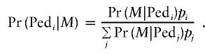For a simple numerical example, consider the pedigree depicted in figure 3, with the two daughters as nonidentical twins. Now imagine a second pedigree with the same phenotypes but with the daughters as identical twins. The first locus is the ABO blood group; its three alleles, A, B, and O, have frequencies in whites of 0.28, 0.06, and 0.66, respectively. The second locus is a codominant marker with four equally frequent alleles. Given an error probability of 0.01 in the uniform error model and a prior probability of 0.462 that same-sex twins are identical, the posterior probability that the twins are identical is 0.911. When we change the second marker genotype of one daughter from 1/4 to 1/3, the posterior probability that the twins are identical becomes 0.023. If genotyping errors were not taken into account, then the posterior probability that the twins are identical would drop to zero. With genotyping errors built into the analysis model, our conclusions are less definite but more secure.

Figure 3.

Determination of twin zygosity

Discussion

Marker genotyping errors are the skeleton in the closet of statistical genetics. It is common knowledge that there is considerable mistyping in most genotype data and that error rates as low as 1%–2% can distort map distances and linkage conclusions (Buetow 1991; Goldstein et al. 1997; Douglas et al. 2000; Abecasis et al. 2001). However, statistical analysis is usually performed under the assumption that all of the genetic data are correct once obvious Mendelian errors have been removed. In fact, Douglas et al. (2002 [in this issue]) show that, for typical multiallelic markers and completely typed four-person nuclear families, ∼40% of the genotyping errors are Mendelian consistent. Furthermore, the fraction of mistypings consistent with Mendelian inheritance will increase with the more widespread use of SNPs and other biallelic markers. The problems are particularly acute in genome scans involving sib pairs without parents (Douglas et al. 2002 [in this issue]). Unfortunately, research studies seldom undertake complete detection of genotyping errors, and, in practice, statisticians almost never explicitly account for errors in their analyses.

We have defined two general pedigree, multipoint algorithms that integrate genotyping errors into likelihood calculations. Perhaps the most useful of our current applications of these algorithms is the calculation of posterior mistyping probabilities at each observed genotype. Our deterministic descent-graph algorithm is exact on small pedigrees. On large pedigrees, our stochastic MCMC algorithm provides an acceptably accurate substitute. All Mendelian errors are found. By analyzing all markers simultaneously, we are able to detect errors revealed by double recombination events between closely spaced markers.

We have several predecessors to thank for clarifying the advantages of posterior error probabilities over rule-based methods of error detection (Ott 1991, 1993; Lincoln and Lander 1992; Ehm et al. 1996; Stringham and Boehnke 1996; O’Connell and Weeks 1998). Our particular contributions to this subject include: (a) the elimination of the unnecessary assumption that one error, at most, occurs per pedigree; (b) the ability to handle pedigrees of nearly unlimited size and complexity; (c) the construction of more-realistic error models; (d) maximum-likelihood estimation of error rates from multilocus data; and (e) the inclusion of error models in the problem of pedigree selection.

Although we have devised an empirical error model that reflects the predominant avenues of mistyping, there is so much variability in genotyping methods and expertise that we consider the less specific uniform-error model as the natural default. In practice, the uniform-error model finds almost all errors (Ehm et al. 1996). Within our programs, it is easy for users to specify their own error rates and their own probability thresholds for the flagging of potential errors. Douglas et al. (2000) give reasons for imposing different thresholds for different markers. Additional error models can be implemented in our programs, with minor coding.

A useful adaptation of the error model would be to carry forward from the typing process any conclusions about the quality of the genotype. If the genotyper or the genotyping software listed a confidence score with each observed genotype, this could be used to inform and improve the error model. Confidence scores can be based on the morphology and intensity of allele bands. Our programs take a small step in this direction by allowing half-typed genotypes to be included in the data files. If there is high confidence at one allele and low confidence at the other, the genotype can be listed as consisting of one specific allele and another unknown allele.

All error models and their predictions are approximations of reality. Nonetheless, we have been heartened to see that most genotypes flagged by our routines represent true typing errors. Exceptions to this rule occur when relatively high posterior error probabilities are distributed over several closely related people. All of the error models we have considered involve independent errors. This simplification may not always hold. In one case, our programs suggested that a single allele was mistyped in a parent. Closer examination of the data showed instead that three alleles were in error in the children. Despite these caveats, we have found that it is best to treat flagged genotypes with great skepticism. At the very least, one should re-examine the original images. If no errors are seen and if resources allow, it is best to retype. When the expense of retyping is prohibitive or samples are not available, we recommend dropping suspect genotypes when performing any statistical analysis that assumes the data are error free. Observed data should never be changed to new, nonblank values solely on the basis of statistical inference; they should be altered only on the basis of laboratory evidence. Missing data are better than bad data, since a loss in power is preferable to false conclusions. Nevertheless, one can be overzealous in the deletion of questionable genotypes. As we have stressed earlier, it would be better to address suspect data within the analysis rather than delete them entirely.

Estimation of error rates has also proven to be a useful tool. In particular, the locus-specific error rates can highlight markers that should be redesigned or replaced. Such optimization of marker sets is crucial for high-efficiency genotyping.

As currently configured, our algorithms do not apply to the genotyping of random individuals in case-control association studies or to sib pair studies without parental data. Errors can be detected in such individuals in two ways. First, pedigree-independent quality-control procedures can be implemented (Ewen et al. 2000; Papp et al. 2000). Such screening is a very valuable initial step, even when pedigrees are available. Second, departures from known patterns of linkage disequilibrium can guide error detection. It may be, for example, that some haplotypes are virtually nonexistent, even though an unjustified assumption of linkage equilibrium would suggest otherwise. Relaxing the assumption of linkage equilibrium is feasible for the MCMC method but not for the deterministic descent-graph method.

Error detection, correction, and integration merit more attention than they have received in the past. We have stressed the need to adapt analysis to allow for genotyping errors. This relieves users of the responsibility of manually determining the correct values of doubtful genotypes. Such software is essential if high-throughput analysis is to match high-throughput data generation. One of the most urgent tasks is to build specialized error models for the new gene-chip technologies. In the near future, we will continue to adapt MENDEL and SimWalk2 to integrate mistyping into more statistical genetic analysis options. The current version of SimWalk2 implements the error models found in the present article in the calculation of posterior mistyping probabilities at each observed genotype. It can be downloaded by visiting the UCLA Human Genetics Web site. The new version of MENDEL is still under development and will be released at the same site, as soon as testing and documentation are complete. We hope that our efforts will stimulate others to develop even better tools addressing these neglected but important problems of genetics.

References

- Abecasis GR, Cherny SS, Cardon LR (2001) The impact of genotyping error on family-based analysis of quantitative traits. Eur J Hum Genet 9:130–134 [DOI] [PubMed] [Google Scholar]
- Akey JM, Zhang K, Xiong M, Doris P, Jin L (2001) The effect that genotyping errors have on the robustness of common linkage-disequilibrium measures. Am J Hum Genet 68:1447–1456 [DOI] [PMC free article] [PubMed] [Google Scholar]
- Angier N (1997) Sex and the female chimp. The New York Times, May 27:C8 [Google Scholar]
- ——— (2001) A fresh look at the straying ways of the female chimp. The New York Times, May 15:F3 [Google Scholar]
- Boehnke M, Cox NJ (1997) Accurate inference of relationships in sib-pair linkage studies. Am J Hum Genet 61:423–429 [DOI] [PMC free article] [PubMed] [Google Scholar]
- Broman KW, Weber JL (1998) Estimation of pairwise relationships in the presence of genotyping errors. Am J Hum Genet 63:1563–1564 [DOI] [PMC free article] [PubMed] [Google Scholar]
- Brzustowicz LM, Mérette C, Xie X, Townsend L, Gilliam TC, Ott J (1993) Molecular and statistical approaches to the detection and correction of errors in genotype databases. Am J Hum Genet 53:1137–1145 [PMC free article] [PubMed] [Google Scholar]
- Buetow KH (1991) Influence of aberrant observations on high-resolution linkage analysis outcomes. Am J Hum Genet 49:985–994 [PMC free article] [PubMed] [Google Scholar]
- Cardon LR, Smith DS, Fulker DW, Kimberling WJ, Pennington BF, DeFries JC (1994) Quantitative trait locus for reading disability on chromosome 6. Science 266:276–279 [DOI] [PubMed] [Google Scholar]
- ——— (1995) Quantitative trait locus for reading disability: correction. Science 268:1553 [DOI] [PubMed] [Google Scholar]
- Cavalli-Sforza LL, Bodmer WF (1971) The genetics of human populations. Freeman, San Francisco [Google Scholar]
- Constable JL, Ashley MV, Goodall J, Pusey AE (2001) Noninvasive paternity assignment in Gombe chimpanzees. Mol Ecol 10:1279–1300 [DOI] [PubMed] [Google Scholar]
- Daw EW, Thompson EA, Wijsman EM (1998) Bias in multipoint linkage analysis arising from map misspecification. Am J Hum Genet Suppl 63:A17 [DOI] [PubMed] [Google Scholar]
- Douglas JA, Boehnke M, Lange K (2000) A multipoint method for detecting genotyping errors and mutations in sibling-pair linkage data. Am J Hum Genet 66:1287–1297 [DOI] [PMC free article] [PubMed] [Google Scholar]
- Douglas JA, Skol AD, Boehnke M (2002) Probability of detection of genotyping errors and mutations as inheritance inconsistencies in nuclear-family data. Am J Hum Genet 70:487–495 (in this issue) [DOI] [PMC free article] [PubMed] [Google Scholar]
- Ehm MG, Kimmel M, Cottingham RW Jr (1996) Error detection for genetic data, using likelihood methods. Am J Hum Genet 58:225–234 [PMC free article] [PubMed] [Google Scholar]
- Ehm MG, Wagner M (1998) A test statistic to detect errors in sib-pair relationships. Am J Hum Genet 62:181–188 [DOI] [PMC free article] [PubMed] [Google Scholar]
- Elston RC, Stewart J (1971) A general model for the genetic analysis of pedigree data. Hum Hered 21:523–542 [DOI] [PubMed] [Google Scholar]
- Ewen KR, Bahlo M, Treloar SA, Levinson DF, Mowry B, Barlow JW, Foote SJ (2000) Identification and analysis of error types in high-throughput genotyping. Am J Hum Genet 67:727–736 [DOI] [PMC free article] [PubMed] [Google Scholar]
- Gagneux P, Woodruff DS, Boesch C (1997) Furtive mating in female chimpanzees. Nature 387:358–359 [DOI] [PubMed] [Google Scholar]
- Goldstein DR, Zhao H, Speed TP (1997) The effects of genotyping errors and interference on estimation of genetic distance. Hum Hered 47:86–100 [DOI] [PubMed] [Google Scholar]
- Gordon D, Heath SC, Ott J (1999a) True pedigree errors more frequent than apparent errors for single nucleotide polymorphisms. Hum Hered 49:65–70 [DOI] [PubMed] [Google Scholar]
- Gordon D, Heath SC, Xin L, Ott J (2001) A transmission/disequilibrium test that allows for genotyping errors in the analysis of single-nucleotide polymorphism data. Am J Hum Genet 69:371–380 [DOI] [PMC free article] [PubMed] [Google Scholar]
- Gordon D, Matise TC, Heath SC, Ott J (1999b) Power loss for multiallelic transmission/disequilibrium test when errors introduced: GAW11 simulated data. Genet Epidemiol 17 Suppl 1:S587–S592 [DOI] [PubMed] [Google Scholar]
- Gordon D, Ott J (2001) Assessment and management of single nucleotide polymorphism genotype errors in genetic association analysis. Pac Symp Biocomput 2001:18–29 [DOI] [PubMed] [Google Scholar]
- Göring HHH, Terwilliger JD (2000a) Linkage analysis in the presence of errors I: complex-valued recombination fractions and complex phenotypes. Am J Hum Genet 66:1095–1106 [DOI] [PMC free article] [PubMed] [Google Scholar]
- ——— (2000b) Linkage analysis in the presence of errors II: marker-locus genotyping errors modeled with hypercomplex recombination fractions. Am J Hum Genet 66:1107–1118 [DOI] [PMC free article] [PubMed] [Google Scholar]
- ——— (2000c) Linkage analysis in the presence of errors III: marker loci and their map as nuisance parameters. Am J Hum Genet 66:1298–1309 [DOI] [PMC free article] [PubMed] [Google Scholar]
- ——— (2000d) Linkage analysis in the presence of errors IV: joint psuedomarker analysis of linkage and/or linkage disequilibrium on a mixture of pedigrees and singletons when the mode of inheritance cannot be accurately specified. Am J Hum Genet 66:1310–1327 [DOI] [PMC free article] [PubMed] [Google Scholar]
- Guo SW, Thompson EA (1992) A Monte Carlo method for combined segregation and linkage analysis. Am J Hum Genet 51:1111–1126 [PMC free article] [PubMed] [Google Scholar]
- Heath SC (1998) A bias in TDT due to undetected genotyping errors. Am J Hum Genet Suppl 63:A292 [Google Scholar]
- Keener JP (1988) Principles of applied mathematics: transformation and approximation. Addison-Wesley, Redwood City, CA [Google Scholar]
- Kruglyak L, Daly MJ, Lander ES (1995) Rapid multipoint linkage analysis of recessive traits in nuclear families, including homozygosity mapping. Am J Hum Genet 56:519–527 [PMC free article] [PubMed] [Google Scholar]
- Kruglyak L, Daly MJ, Reeve-Daly MP, Lander ES (1996) Parametric and nonparametric linkage analysis: a unified multipoint approach. Am J Hum Genet 58:1347–1363 [PMC free article] [PubMed] [Google Scholar]
- Kruglyak L, Lander ES (1998) Faster multipoint linkage analysis using Fourier transforms. J Comput Biol 5:1–7 [DOI] [PubMed] [Google Scholar]
- Kumm J, Browning S, Thompson EA (1999) Validation of pedigree data in the presence of genotyping error. Am J Hum Genet Suppl 65:A208 [Google Scholar]
- Lander ES, Green P (1987) Construction of multilocus linkage maps in humans. Proc Natl Acad Sci USA 84:2363–2367 [DOI] [PMC free article] [PubMed] [Google Scholar]
- Lange K (1997) Mathematical and statistical methods for genetic analysis. Springer-Verlag, New York [Google Scholar]
- Lange K, Boehnke M, Weeks DE (1988) Programs for pedigree analysis: MENDEL, FISHER, and dGENE. Genet Epidemiol 5:471–472 [DOI] [PubMed] [Google Scholar]
- Lange K, Matthysse S (1989) Simulation of pedigree genotypes by random walks. Am J Hum Genet 45:959–970 [PMC free article] [PubMed] [Google Scholar]
- Lange K, Sobel E (1991) A random walk method for computing genetic location scores. Am J Hum Genet 49:1320–1334 [PMC free article] [PubMed] [Google Scholar]
- Lathrop GM, Hooper AB, Huntsman JW, Ward RH (1983) Evaluating pedigree data. I. The estimation of pedigree error in the presence of marker mistyping. Am J Hum Genet 35:241–262 [PMC free article] [PubMed] [Google Scholar]
- Lincoln SE, Lander ES (1992) Systematic detection of errors in genetic linkage data. Genomics 14:604–610 [DOI] [PubMed] [Google Scholar]
- Lunetta KL, Boehnke M, Lange K, Cox DR (1995) Experimental design and error detection for polyploid radiation hybrid mapping. Genome Res 5:151–163 [DOI] [PubMed] [Google Scholar]
- McPeak MS, Sun L (2000) Statistical tests for detection of misspecified relationships by use of genome-screen data. Am J Hum Genet 66:1076–1094 [DOI] [PMC free article] [PubMed] [Google Scholar]
- Nijenhuis A, Wilf HS (1978) Combinatorial algorithms for computers and calculators. 2d ed. Academic Press, New York [Google Scholar]
- O’Connell JR, Weeks DE (1998) PedCheck: a program for identification of genotype incompatibilities in linkage analysis. Am J Hum Genet 63:259–266 [DOI] [PMC free article] [PubMed] [Google Scholar]
- ——— (1999) An optimal algorithm for automatic genotype elimination. Am J Hum Genet 65:1733–1740 [DOI] [PMC free article] [PubMed] [Google Scholar]
- Ott J (1977) Linkage analysis with misclassification at one locus. Clin Genet 12:110–124 [DOI] [PubMed] [Google Scholar]
- ——— (1991) Analysis of human genetic linkage. Revised ed. Johns Hopkins University Press, Baltimore [Google Scholar]
- ——— (1993) Detecting marker inconsistencies in human gene mapping. Hum Hered 43:25–30 [DOI] [PubMed] [Google Scholar]
- Papp JC, Kearsey G, Lange K (2000) Improving the quality of genotyping data. Am J Hum Genet Suppl 67:A1658 [Google Scholar]
- Sieberts S, Wijsman EM, Thompson EA (2001) Relationship inference from trios of individuals in the presence of typing error. Am J Hum Genet Suppl 69:A1357 [DOI] [PMC free article] [PubMed] [Google Scholar]
- Smith HF (1937) Test of significance for Mendelian ratios when classification is uncertain. Ann Eugen 8:94–95 [Google Scholar]
- Sobel E, Lange K (1993) Metropolis sampling in pedigree analysis. Stat Methods Med Res 2:263–282 [DOI] [PubMed] [Google Scholar]
- ——— (1996) Descent graphs in pedigree analysis: applications to haplotyping, location scores, and marker-sharing statistics. Am J Hum Genet 58:1323–1337 [PMC free article] [PubMed] [Google Scholar]
- Stringham HM, Boehnke M (1996) Identifying marker typing incompatibilities in linkage analysis. Am J Hum Genet 59:946–950 [PMC free article] [PubMed] [Google Scholar]
- Terwilliger JD, Weeks DE, Ott J (1990) Laboratory errors in the reading of marker alleles cause massive reductions in lod score and lead to gross overestimates of the recombination fraction. Am J Hum Genet Suppl 47:A201 [Google Scholar]
- Thompson EA (1975) The estimation of pairwise relationships. Ann Hum Genet 39:173–188 [DOI] [PubMed] [Google Scholar]
- ——— (1986) Pedigree analysis in human genetics. Johns Hopkins University Press, Baltimore [Google Scholar]
- ——— (1994) Monte Carlo likelihood in genetic mapping. Stat Sci 9:355–366 [DOI] [PubMed] [Google Scholar]
- ——— (1996) Likelihood and linkage: from Fisher to the future. Ann Stat 24:449–465 [Google Scholar]
- Weir BS (1996) Genetic data analysis II. Sinauer, Sunderland, MA [Google Scholar]