

Abstract
We present a Bayesian, Markov-chain Monte Carlo method for fine-scale linkage-disequilibrium gene mapping using high-density marker maps. The method explicitly models the genealogy underlying a sample of case chromosomes in the vicinity of a putative disease locus, in contrast with the assumption of a star-shaped tree made by many existing multipoint methods. Within this modeling framework, we can allow for missing marker information and for uncertainty about the true underlying genealogy and the makeup of ancestral marker haplotypes. A crucial advantage of our method is the incorporation of the shattered coalescent model for genealogies, allowing for multiple founding mutations at the disease locus and for sporadic cases of disease. Output from the method includes approximate posterior distributions of the location of the disease locus and population-marker haplotype proportions. In addition, output from the algorithm is used to construct a cladogram to represent genetic heterogeneity at the disease locus, highlighting clusters of case chromosomes sharing the same mutation. We present detailed simulations to provide evidence of improvements over existing methodology. Furthermore, inferences about the location of the disease locus are shown to remain robust to modeling assumptions.
Introduction
Fine-scale linkage disequilibrium (LD) mapping using high-density marker maps is widely recognized as having the potential to play a major role in the identification of genes involved in complex diseases. In particular, a detailed single-nucleotide polymorphism (SNP) map of the human genome has recently been unveiled (International Human Genome Sequence Consortium 2001; International SNP Map Working Group 2001), and there is currently an exciting period of development of efficient statistical methods needed to meet the challenges posed by LD mapping with this type of data.
The simplest approaches, based on analysis of markers one at a time, are readily seen to be statistically inefficient. The likelihood methods of Terwilliger (1995), Xiong and Guo (1997), and Collins and Morton (1998) combine information across markers but do so via an assumption of independence. This assumption is invalid, since alleles at closely linked loci are often strongly correlated, and it will obviously give rise to misleading inferences (Clayton 2000; Rannala and Slatkin 2000). Recently, genuinely multipoint methods that model complete marker haplotypes have begun to appear. These include the methods of McPeek and Strahs (1999), Morris et al. (2000), Rannala and Reeve (2001), and Liu et al. (2001). Some of the principal features of these LD-mapping methods, to be discussed further below, are summarized in table 1.
Table 1.
Summary of Model Assumptions for Various Existing Methods of Fine-Scale Mapping via Population-Based Disease-Marker Association
| Method | Structure of Tree | Likelihood | Estimation Procedure | Ancestral Marker Haplotype | Marker Mutation | κ |
| Terwilliger (1995) | Star shaped | Composite over each marker | Integrated maximum likelihood | Integrate over complete distribution | Assumed to be 0 | Assumed to be 1 cM = 1 Mb |
| Xiong and Guo (1997) | Star shaped | Composite over each marker | Maximum likelihood | Assumed to be known | Assumed to be 0 | Assumed to be 1 cM = 1 Mb |
| Collins and Morton (1998) | Star shaped | Composite over each marker | Maximum likelihood | Assumed to be known (preanalysis) | Estimated in Malecot model | Estimated in Malecot model |
| McPeek and Strahs (1999) | Star shaped, corrected for pairwise correlation | Complete marker haplotype | Maximum likelihood | Integrate over “restricted” distribution | Assumed to be known | Assumed to be 1 cM = 1 Mb |
| Morris et al. (2000) | Star shaped, corrected for pairwise correlation | Complete marker haplotype | Bayesian | Integrate over complete distribution | Assumed to be known | Variable across region |
| Rannala and Reeve (2001) | Bifurcating genealogy | Complete marker haplotype | Bayesian | Integrate over complete distribution | Assumed to be known | Assumed to be 1 cM = 1 Mb |
| Liu et al. (2001) | Star shaped, corrected for pairwise correlation | Complete marker haplotype | Bayesian | Integrate over complete distribution | Assumed to be known | Assumed to be 1 cM = 1 Mb |
| Shattered coalescent | Shattered bifurcating genealogy | Complete marker haplotype | Bayesian | Integrate over complete distribution | Assumed to be known | Assumed to be κ cM = 1 Mb |
The key idea underlying all LD-mapping methods is that, in the vicinity of a disease locus, a sample of case chromosomes will tend to have more-recent shared ancestry than do control chromosomes, because many of them may share a recent disease mutation. Consequently, a sample of case chromosomes is expected to display excess sharing of marker alleles over control chromosomes, the excess decaying with distance from the disease locus. However, this simple situation is often complicated by multiple disease mutations, sporadics among the sample of case chromosomes, mutations at marker loci, and allele sharing due to population substructure or founder effects. The challenge for LD mapping is to efficiently detect excess allele sharing due to shared inheritance of a common disease mutation and to distinguish it from background patterns of variation. This in turn requires effective modeling of the mechanisms generating allele sharing and the resulting LD.
Figure 1 illustrates the complex allele-sharing structure that may arise in the chromosome region flanking a disease locus, even in a simplified setting that ignores the complicating factors listed above. In this figure, a possible genealogical tree for the disease locus, x, is presented for a sample of eight chromosomes, represented by the vertical bars C1–C8; the horizontal bars correspond to ancestral chromosomes, which are not generally observed. The dark shading in both the horizontal and the vertical bars indicates chromosome segments inherited, identical by descent (IBD), from the ancestral chromosome at the root of the tree (fig. 1, top), the most recent common ancestor (MRCA) of the sample at locus x. Since mutations are rare, an observed chromosome will usually bear the same allele as does the MRCA, at any marker locus within the preserved (i.e., shaded) region. Notice that a boundary of the preserved region is often the same for closely related chromosomes, such as C1 and C2. This is because the common boundary is due to the same historical recombination event. Such chromosome pairs will also tend to share any marker mutations arising since the MRCA. Thus, closely related chromosomes may also share with each other, in the vicinity of x, a chromosome segment larger than that shared with the MRCA.
Figure 1.

Genealogical tree representing shared ancestry, at locus x, of a sample of eight chromosomes, C1–C8. The descent of the founder chromosome segment, indicated by the blackened regions, is disrupted by historical recombination events. Since mutation events are rare, an observed chromosome will usually bear the same allele as the founder, at any marker locus within the preserved region.
Unfortunately, the genealogical tree underlying a sample of chromosomes at a given locus is usually unknown, and its structure must be either assumed or inferred. Many existing methods for LD mapping (Terwilliger 1995; Xiong and Guo 1997; Collins and Morton 1998) assume a “star-shaped” tree, in which case chromosomes have descended independently from their MRCA. By ignoring the pattern of shared ancestry among case chromosomes, the star-genealogy assumption leads to overoptimism. For example, a shared recombination or marker-mutation event in the genealogical history of two or more case chromosomes may be interpreted as distinct events, with their information multiply counted. As a result, the variance of parameter estimates, including the location of the disease locus, tends to be understated and may yield misleading inferences.
The inadequacy of the star-genealogy assumption has been recognized by McPeek and Strahs (1999). They make allowance for the correlation, in allele sharing, between case chromosomes in a quasi-likelihood framework (Wedderburn 1974; McCullagh and Nelder 1989). Their quasi–log likelihood is of the same functional form as that under a star genealogy but is multiplied by a correction factor, dependent only on the sample frequency of case chromosomes. A weakness of this approach, also employed by Morris et al. (2000), is that the correlation is the same for each pair of case chromosomes, regardless of the available marker information.
Lam et al. (2000) construct a genealogical tree for chromosomes bearing a common mutation at the disease locus, using a combination of parsimony and likelihood methods. They then proceed as if the tree is known with certainty and is the same for all putative locations for the disease locus. Graham and Thompson (1998) integrate over trees consistent with the case chromosomes, generated under a Moran (1962) model with known demographic parameters, but their method is currently restricted to interval mapping with pairs of marker loci. Rannala and Reeve (2001) use Markov-chain Monte Carlo (MCMC) methods in a Bayesian framework, to integrate over genealogical trees generated under an intra-allelic coalescent model (Slatkin and Rannala 1997).
Here, we present a Bayesian multipoint method for fine-scale LD mapping, a method that also employs MCMC technology and coalescent theory to average over possible genealogies underlying the sample of case chromosomes. However, there are a number of key distinctions between our new method and that of Rannala and Reeve (2001). Perhaps the major advantage of our method is that we introduce a shattered-coalescent model for genealogies, allowing both for (a) multiple founding disease mutations at the same locus, and (b) sporadic cases of disease, caused by environmental factors or mutations at other loci. Liu et al. (2001) also allow for multiple mutations, at the same locus, in a Bayesian MCMC framework. However, they assume that each cluster of case chromosomes bearing the same disease mutation descends from the founder for that mutation, under a star genealogy. An additional advantage over the method of Rannala and Reeve (2001) is that we allow for background LD between marker loci. We follow Liu et al. (2001) by modeling control marker–haplotype frequencies via a first-order Markov process.
In contrast to Rannala and Reeve (2001), we choose not to incorporate prior information about candidate genes, available from an annotated human genome sequence and from disease-mutation databases. We prefer to investigate only the information contained in the marker haplotypes of the sample of case and control chromosomes. Other sources of information may be incorporated later, when the results of our analysis are interpreted. It is a feature of the Bayesian paradigm for statistical inference that the order in which independent sources of data are processed does not affect final inferences.
In addition to their approaches to modeling the genealogy underlying a sample of case chromosomes, another key feature differentiating methods for multipoint LD mapping is their treatment of the founding marker haplotype (table 1). Xiong and Guo (1997) assume this information to be known. Collins and Morton (1998) estimate the most likely ancestral allele at each marker locus but then treat the resulting haplotype as if it is, with certainty, known to be the founder. Clayton (2000) recognizes that it is more appropriate to treat the founding haplotype as missing data and to integrate over a suitable probability distribution in likelihood calculations. In the composite-likelihood framework, Terwilliger (1995) integrates over all possible alleles at each marker locus. However, this approach is likely to be computationally demanding for genuinely multipoint methods. McPeek and Strahs (1999) overcome this problem by considering only a restricted set of marker haplotypes, deemed most likely to be the founder, using a branch-and-bound algorithm. Here, we follow Morris et al. (2000), Liu et al. (2001), and Rannala and Reeve (2001), by integrating approximately over ancestral marker haplotypes in an MCMC framework.
We have conducted a detailed simulation study to compare our method with rival approaches. We present results that provide evidence of improvements made by our new method, in terms of mean square error and the coverage of credibility intervals for the location of the disease locus. In addition, inferences about location are shown to remain robust to modeling assumptions.
Methods
We consider a candidate region that is assumed to include a unique disease-susceptibility locus at unknown location x. The region is spanned by marker loci, with unknown background population-haplotype proportions denoted “h.” A sample of nA unrelated affected case chromosomes and nU unrelated unaffected control chromosomes are typed at the marker loci, to obtain sets of haplotypes A and U, respectively. A summary of notation is presented, for reference, in Appendix A.
Our goal is to approximate  , the posterior probability density function of x, given the marker haplotype data. The elements of h are nuisance parameters, not of primary interest but necessary to evaluate
  . Thus, we first consider the joint posterior density of x and h, which, by Bayes’s theorem, can be written as
For convenience, we use “P” to denote posterior densities of parameters, given data; “L”to denote likelihoods of data, given parameters; and “π” to denote unconditional prior densities.
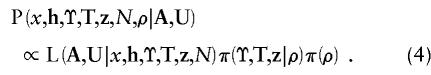
Below, we assume a uniform prior for x, although it is straightforward to employ an informative prior as do Rannala and Reeve (2001). We also assume (a) that the haplotype proportions across the marker loci are jointly uniform a priori, subject to the constraint that they sum to one, and (b) that h is independent of x. Therefore,  is constant and can be omitted from posterior probability density function (1).
The marginal posterior density for x can be recovered from posterior probability density function (1) by integration over haplotype proportions, h,
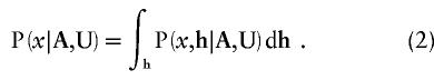 |
This integration can be approximated by MCMC methods by sampling from the distribution of  and simply ignoring the values of h.
Clearly, the likelihood, L , arising in posterior probability density function (1), cannot be calculated directly but, instead, requires the introduction of additional parameters, M, describing the mechanisms generating the observed sample of marker haplotypes from the founding disease mutation event(s), including the genealogical tree underlying the sample of case chromosomes at x. The joint posterior probability density function can then be written
in which we have assumed prior independence of M, h, and x. The marginal posterior distribution for x—or for any of the other model parameters—can be obtained by integrations or summations analogous to posterior probability density function (2).
The Shattered Coalescent Model for Genealogical Trees
We assume initially that the sample of case chromosomes shares a recent common ancestor bearing a disease mutation at locus x. The descent of the sample from this common ancestor is then represented by means of a bifurcating genealogical tree with topology (branching pattern) T and branch lengths ϒ (fig. 2). The most successful class of prior probability models for  is given by the coalescent process (Kingman 1982; Hudson 1991; Donnelly and Tavaré 1995; Nordborg 2001). Under this model, each topology T is equally likely, with the leaf nodes regarded as labeled to avoid combinatorial complications. Time is scaled to be measured in units of N generations, where N is the effective population size of chromosomes. Under the standard-coalescent model, the scaled time, wk, during which the tree has exactly k distinct lineages, has an exponential distribution with rate parameter λk=[k(k-1)]/2, independently for each k. These coalescence times then determine the branch lengths, ϒ, of the genealogical tree, as illustrated by figure 2.
Figure 2.

Parameterization of the genealogical tree in terms of the waiting times, wk, between coalescent events, during which the tree has exactly k distinct lineages. The length of a branch is given by the sum of waiting times between the offspring node and parental node; for example, the length of the branch above node 1 is given by τ1=w8+w7, and the length of the branch above node 2 is given by τ2=w5+w4+w3.
The standard-coalescent model can be derived under the assumption that the leaves of the tree correspond to a random sample of chromosomes ascertained from a large random-mating population of constant size N, not subject to selection at the disease locus x. However, these assumptions are unlikely to hold, even approximately, for the sample of case chromosomes. One problem is the ascertainment process: for population-based association studies, the sample is enriched for case chromosomes because the disease is often rare and too few affecteds would be included in a random sample of a population. This affects the time scale of genealogical trees, which can be accommodated by absorption into N, but it also affects the shape of the tree (Slatkin 1996; Wiuf and Donnelly 1999). Nevertheless, the standard-coalescent process incorporates the principal effects of shared ancestry, providing a relatively weak prior-probability model that is readily “overwhelmed” by the data.
Rannala and Reeve (2001) propose, instead, the use of the intra-allelic coalescent process (Slatkin and Rannala 1997) as an “appropriate” prior model for the distribution of genealogical trees underlying the sample of case chromosomes. However, their model requires specification of the age of the disease mutation, which is unlikely to be known. Further concerns as to the suitability of this model, particularly for mutations with low relative population frequency, are raised by Wiuf and Donnelly (1999). Perhaps a more important limitation of the intra-allelic coalescent model is the assumption that all case chromosomes descend from the same founding mutation event, represented by a single genealogy. Even for Mendelian disorders, sporadic cases of disease are commonly observed, and singleton founding-mutation events are the exception and not the rule (Pennisi 1998).
To overcome this problem, we generalize the coalescent process to allow branches of the genealogical tree to be removed—hence the term “shattered” coalescent model—by introducing a vector of indicator variables, z, defined as
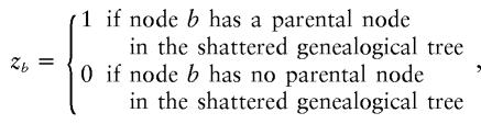 |
over all leaf nodes and internal nodes of the tree. A realization of this process is illustrated in figure 3. Singleton leaf nodes with zb=0 correspond to sporadic case chromosomes (phenocopies) bearing the more ancient, normal allele at locus x. Disconnected subtrees, in which zb=0 for an internal node of the tree, correspond to founders for independent disease-mutation events at locus x.
Figure 3.

Realization of the shattered coalescent process from an unshattered genealogy underlying a sample of 16 case chromosomes. The branches indicated by dashed lines are removed from the unshattered genealogy by setting the indicator variable, zb=0, for their offspring nodes (top). The resulting shattered genealogy (bottom) yields two unrelated subtrees, each corresponding to independent mutations at the disease locus, and two sporadic case chromosomes.
The shattered coalescent process does not explicitly address the problems of ascertainment. However, below we present data analyses and simulation studies to provide evidence that inferences about x are robust to these modeling assumptions. Under this model for the prior distribution of genealogies underlying the sample of case chromosomes,
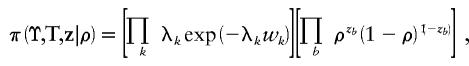 |
where the products are over coalescence times, k, and nodes, b. Under this model, each node has, independently, probability ρ of having a parent node in the genealogical tree. A low value of ρ corresponds to a high level of genetic heterogeneity at x among case chromosomes, with many singleton leaves and small clusters in the genealogy. Higher values of ρ often lead to a single major subtree, with the standard-coalescent process recovered for ρ=1. We assume a Beta(2,1) distribution, a priori, for the shattering parameter, ρ, given by  .
.
Assignment of an informative prior to N is difficult, because the interpretation of this parameter is not clear in the context of the ascertainment problem. Thus, we take π(N) to be both uniform over a wide interval and independent of the genealogical tree. Posterior probability density function (3) can then be written as
 |
Augmenting the Data
The likelihood  arising in posterior probability density function (4) could be calculated directly but would require summation over all possible configurations of marker haplotypes at internal nodes of the genealogical tree, denoted “I.” This computationally demanding summation can be avoided by treating I as augmented data. In brief, within an MCMC framework, we simulate over possible values for the augmented data, in the same way as for the model parameters described above, according to the appropriate posterior distribution. Missing marker information at leaf nodes can be easily treated in the same way, by simulating over the possible values for untyped alleles, according to the appropriate posterior probability distribution.
Extending posterior probability density function (4) further, to incorporate augmented data and missing marker information, we obtain an expression for the target posterior density,
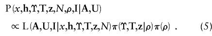 |
The key advantage of posterior probability density function (5) over posterior probability density function (4) is that  is readily calculated, as we now describe.
Computing the Likelihood
Most of our attention has been focused on modeling the genealogy of the sample of case chromosomes, at x. The control chromosomes are also affected by their genealogical history. However, since these chromosomes do not share a recent disease mutation, their shared ancestry is expected to extend much farther into the past than that of the case chromosomes, an expectation that is supported, below (see the “Relative Depth of Case and Control Genealogies” subsection), by simulation. The effects of shared ancestry among the sample of control chromosomes are thus less important, and we adopt a more simple model. We assume that, given h, the set of control marker haplotypes, U, is independent of the other data and model parameters, so that
The most trivial model for L assumes no LD in the population of normal chromosomes, with the likelihood contribution of each control chromosome given by the product of population proportions, p, for the constituent marker alleles. We consider a more realistic model for L
 , also incorporating an LD parameter, Δ, between each pair of adjacent marker loci, via a first-order Markov process (Liu et al. 2001).
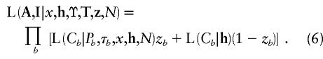
For the sample of case chromosomes, consider a particular node, b, of the underlying genealogy, bearing marker haplotype Cb. We consider two scenarios:
-
1.
Node b has no parent node in the underlying genealogy, zb=0, corresponding either to a founder for a disease mutation at x (i.e., internal node) or to a sporadic case (i.e., leaf node). Founding mutation events and sporadic cases are assumed to occur on random chromosomes from the population and thus can be modeled in the same way as control marker haplotypes.
-
2.
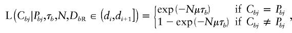
Node b has a parent node in the underlying genealogy, indicated by zb=1. The distribution of Cb now depends on both the marker haplotype of the parental node, Pb, and the occurrence of recombination and marker-mutation events along the connecting branch, of length τb (scaled coalescent time units).
Recombination and marker-mutation events are assumed to occur independently across the branches of the tree, so that
 |
Conditional on the marker haplotype of the parental node, Pb, the distribution of Cb is determined by the location, relative to the disease locus, of the nearest recombination event (NRE), on either side of x. The haplotype between the two NREs will be preserved from the parental node to the offspring node, unless mutation events occur at the marker loci. The haplotype extending beyond the preserved region, on either side of x, is assumed to have occurred as a result of recombination with a random chromosome from the population. Case chromosomes are assumed to be sufficiently rare that the possibility of recombination between two ancestral chromosomes bearing a disease mutation at x can be neglected. Thus, in nonpreserved regions, marker haplotypes are modeled independently according to the population allele proportions and first-order LD parameters, p and Δ, in the same way as control chromosomes. The problem here is that the locations of the NREs on either side of x are unknown. Calculation of the likelihood thus requires, as detailed in Appendix B, summation over all intermarker intervals that are possible locations of the NREs, according to appropriate models for the processes of recombination and marker mutation.
Recombination events are assumed to occur at a rate Nκ per Mb, per scaled unit of coalescent time, a rate that is assumed to be constant both over time and across the candidate region. Thus, the probability of no recombination in a region of y Mb along a branch of length τ is approximated by  . Although recombination rates may vary across the candidate region, we regard this uniform assumption as providing an appropriate, weak prior model for the location of recombination breakpoints, which can be easily overtaken by the data. Mutation is assumed to occur at a rate Nμ per locus, per scaled unit of coalescent time, a rate that, again, is assumed to be constant over time and across loci in the candidate region. Thus, the probability of no mutation along a branch of length τ at a given marker locus is approximated by
  . Subsequently, both κ and μ are assumed to be known constants, obtained from genetic and physical maps of the region and from an understanding of the marker mutation process. These rates could be incorporated as parameters to be estimated. However, the likelihood depends only on the products Nκ and Nμ, so that κ and μ cannot, in practice, be estimated if N is unknown.
Metropolis Algorithm
We have developed an MCMC algorithm of the Metropolis type (Metropolis et al. 1953), to approximate posterior probability density function (5). Let “𝒮” denote the set of unknown parameters and augmented data,  , and let “𝒟” denote the observed marker-haplotype data,
  , so that the target posterior distribution can be written as P
 . At each step of the algorithm, a candidate new value 𝒮′ is proposed, and is accepted in place of 𝒮, with probability
  . If 𝒮′ is not accepted, then the current value 𝒮 is retained. The posterior probabilities can be calculated from posterior probability density function (5), except for a normalizing constant. However, since this constant cancels in the ratio, it is not required; this is one of the principal advantages of a Metropolis algorithm.
The algorithm is run for an initial burn-in period, to allow it to “forget” the randomly selected starting value of 𝒮. Subsequently, each state of 𝒮 accepted by the algorithm represents a random draw from the target posterior distribution. Although these draws will, in general, be correlated, the correlation can be reduced by taking only every rth output, for some suitably large r. The choice of proposal mechanism for the generation of 𝒮′ from 𝒮 is subject to only weak restrictions to ensure validity of the algorithm. However, computational efficiency can be greatly affected by this choice. The multistep proposal procedure used here is summarized in Appendix C.
Interpretation of output from the algorithm is extremely straightforward: to approximate the probability that the unknown 𝒮 lies in some set ℛ, we calculate the proportion of MCMC outputs that lie in ℛ. If ℛ involves only some of the parameters, then the calculated proportion involves only the corresponding columns of the MCMC output.
We have emphasized x as being the primary parameter of interest, but our algorithm generates approximations to many other unknowns which may be of practical use. These include the marker-allele–population proportions and the background LD parameters. For missing marker information, an approximate posterior distribution for each untyped allele can be extracted from the output. In addition, the posterior probability that any pair of case chromosomes shares the same disease mutation can be approximated by the proportion of outputs in which they appear in the same subtree of the shattered genealogy. On the basis of a standard hierarchical clustering algorithm with average linkage (Hartigan 1975), these probabilities can be used to construct a cladogram representing genetic heterogeneity at the disease locus, from which clades of chromosomes bearing the same mutation can be identified. Furthermore, the mean time since the MRCA of each pair of case chromosomes within the same clade can be estimated. With the same type of algorithm, these times can be used to construct a consensus subtree, representing a point estimate of the underlying genealogy of the shared mutation at the disease locus.
The Metropolis algorithm developed here has been implemented in the program COLDMAP, available as UNIX or LINUX executables. The software and accompanying documentation is available, on request, from the corresponding author (A.P.M.).
Simulation Study
We present some of the results of a detailed simulation study designed to compare the performance of our Metropolis algorithm with that of existing methods, which do not explicitly model the genealogy underlying the sample of case chromosomes. The study allows us to check the validity of a number of model assumptions, including robustness to ascertainment and the effects of relatively high rates of sporadic-case chromosomes. We have not considered the case of multiple disease mutations at the same locus. In this setting, we would expect both our method, proposed here, and that of Liu et al. (2001) to outperform existing methods.
To make a fair and direct comparison with our proposed method, denoted “TREE,” we reformulate versions of existing methodology, in a Bayesian MCMC framework. Our Metropolis algorithm is then adapted to estimate the target posterior distribution of the same set of model parameters, outlined below, for each method. The methods considered here are denoted “COMP,” “STAR,” “PAIR,” and “LIU,” each developed under the assumption of a star genealogy. Under this model, the topology of the tree, T, is fixed, with all branch lengths equal to τ, say. Likelihood (6) is then replaced by
 |
where the product is over all leaf nodes of the star genealogy, I is the marker haplotype borne by the single internal node of the tree, and G≡Nτ is the number of generations since this founder. Full details of the likelihood expressions for the four methods are presented in Appendix D.
The method COMP is based on a composite likelihood, assuming the marker loci to be independent. It can be thought of as a fully Bayesian implementation of the method of Terwilliger (1995), allowing for mutation at the marker loci. PAIR and STAR are the same as methods presented by Morris et al. (2000), based on a likelihood for complete marker haplotypes, except that the recombination rate, κ, is assumed to be fixed. The method PAIR incorporates the correction factor proposed by McPeek and Strahs (1999), accounting for the pairwise correlation between case-marker haplotypes resulting from recent shared ancestry.
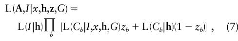
For each of these three methods, the star genealogy is assumed to be unshattered, not explicitly permitting genetic heterogeneity at the disease locus among case chromosomes. However, these methods overcome this problem by incorporating a heterogeneity parameter, φ, corresponding to the probability that a case chromosome bears the disease mutation at x. Under this model, zb=φ in equation (7), for each case chromosome b. Within the Bayesian framework, we approximate the posterior distribution of φ on the basis of the MCMC output, assuming a Beta(2,1) prior probability distribution.
The disadvantage of this approach to dealing with genetic heterogeneity is that the same probability, φ, of bearing the disease mutation is assigned to each case chromosome, regardless of the observed marker haplotype. This is in contrast to the method, LIU, presented by Liu et al. (2001). Although the likelihood expression L is the same as that for STAR, the parameter zb is not assumed to be fixed across case chromosomes. As in the shattered coalescent model, z represents a vector of indicator variables, where zb takes the value 1 if case chromosome b bears the disease mutation at the disease locus and takes the value 0 otherwise. On the basis of the output of the MCMC algorithm, the posterior probability P
 is estimated, independently for each leaf node of the star genealogy. As with our shattered coalescent model, we assume
  for the method LIU, given a Beta(2,1) prior probability distribution for ρ.
We have not included comparisons with the method of Rannala and Reeve (2001), since these authors do not allow for genetic heterogeneity at the disease locus, at any level, among the sample of case chromosomes. Their method is expected to have properties similar to those of TREE, but only for samples of case chromosomes that are genetically homogeneous at the disease locus.
For the methods COMP, STAR, and PAIR, no LD is assumed in the background population of chromosomes. Thus, control marker haplotypes are modeled by the product of constituent population allele proportions, p. In contrast, a first-order Markov process is used to model control marker haplotypes for the methods LIU and TREE, which requires additional pairwise LD parameters Δ.
Data Generation via the Ancestral Recombination Graph
Consider a 2.25-Mb candidate region for a disease locus, spanned by 10 equally spaced SNPs. We investigate the effects that the recombination rate, κ, and the relative frequency of the disease mutation in the population, q, have on inferences that the five methods make about location (table 2).
Table 2.
Summary of Parameter Values for Simulation Study
|
Mean Time to MRCAa(generations) |
||||
| Parameter Set | κ | q | 50 Cases | 50 Controls |
| 1 | .01 | .01 | 161.8 | 19,604.4 |
| 2 | .02 | .01 | 173.4 | 19,244.5 |
| 3 | .01 | .025 | 387.7 | 20,151.8 |
| 4 | .02 | .025 | 392.0 | 19,073.6 |
Based on 1,000 replicates of coalescent process with recombination, for a population of 10,000 chromosomes.
For each replicate, the location of the disease locus is generated at random from within the candidate region. We have developed an algorithm to simulate the joint ancestry of the 10 SNPs and the disease locus, for a population of 10,000 chromosomes, under the standard-coalescent process with recombination (Hudson 1983; Griffiths and Marjoram 1996, 1997), assuming a fixed recombination rate of κ Morgans per Mb across the candidate region. For each SNP, we select at random the position of a single mutation event in the ancestral recombination graph, subject to the constraint that the relative frequency of the mutation must lie in the interval [0.1,0.9] in the population of 10,000 chromosomes. This reflects the nonascertainment of rare SNPs. For the disease locus, we select at random the position of a single mutation event in the ancestral recombination graph, subject to the constraint that q is the relative frequency of the mutation in the population of 10,000 chromosomes. We then select a sample of 50 case chromosomes from the leaves of the ancestral recombination graph that bear the mutation at the disease locus; similarly, a sample of 50 control chromosomes is selected from the leaves of the ancestral recombination graph that do not bear the disease mutation.
For each replicate, the true location of the disease locus is recorded, together with both the time to the MRCA of the sample of case chromosomes and the time to the MRCA of the sample of control chromosomes. Approximations to the posterior distribution of location are then obtained from the output of the Metropolis algorithm for each of the five methods, starting from the same random parameter configuration. For each method, a mutation rate of μ=5×10⁻⁵ per locus, per generation, is assumed for analysis. The median estimate of location is then extracted from the approximate posterior distribution, together with 50% and 95% credibility intervals.
Relative Depth of Case and Control Genealogies
Table 2 presents the mean time (in generations) to the MRCAs of the sample of 50 case chromosomes and 50 control chromosomes, for 1,000 replicates of the coalescent process with recombination under parameter sets 1–4. For a disease mutation with relative population frequency q⩽0.025, the height of the case genealogy is several orders of magnitude less than that of the control genealogy. This would appear to provide support for our choice to neglect the shared ancestry of control chromosomes and to focus, instead, on the genealogy underlying the sample of case chromosomes, at least for relatively rare disease mutations.
Bias and Mean Square Error of Estimated Location
Unbiased estimates of the location of the disease locus were obtained for all five methods, over parameter sets 1–4 (results not presented). Figure 4 presents the mean square error associated with these estimates for the five methods, over 1,000 replicates of the coalescent process with recombination. For all five methods, an increase in the recombination rate κ results in reduced mean square error associated with estimated location. This would be expected, since an increased frequency of recombination events will narrow down the preserved founder marker haplotype in the vicinity of the disease locus, increasing the accuracy of the estimate of location. A similar reduction in mean square error is observed for an increase in the relative population frequency q. This is due to the fact that a more common disease mutation tends to have a more ancient MRCA (table 2), providing greater opportunity for recombination events to occur in the descent of the sample of case chromosomes.
Figure 4.

Mean square error of estimates of the location of the disease locus for parameter sets 1–4, defined in table 2, for five methods of fine-scale LD mapping. COMP = composite likelihood under unshattered star genealogy; STAR = multipoint likelihood under unshattered star genealogy; PAIR = multipoint likelihood under pairwise model of correlation; LIU = multipoint likelihood under shattered star genealogy; TREE = multipoint likelihood with explicit modeling of shattered genealogy.
COMP consistently has the highest mean square error. For parameter sets 1–3, there is little difference between the mean square errors observed for STAR, PAIR, LIU, and TREE. For these parameter sets, the probability of recombination within the candidate region, in the descent of the sample of case chromosomes from their MRCA, is relatively low. As a result, many of the simulated case marker haplotypes are identical, a situation for which the star genealogy is a reasonable fit. However, for parameter set 4, there is greater opportunity for recombination in the candidate region, resulting in greater variability in simulated case marker haplotypes within replicates. In this setting, a bifurcating genealogy is a better fit than a star-shaped tree, and, in terms of mean square error, there some gains for PAIR but more noticeable improvements for TREE.
Coverage of Credibility Intervals for Location
Figure 5 presents, for the five methods, the coverage of 50% and 95% credibility intervals for the location of the disease locus, over 1,000 replicates of the coalescent process with recombination under parameter sets 1–4. The coverage of COMP, STAR, and LIU is too low, at ∼40%–60% of the correct coverage probability. Since the estimates of the location of the disease locus are unbiased, this corresponds to credibility intervals that are too narrow, resulting from the overconfidence incurred by ignoring the structure of the underlying genealogical tree. Coverage of PAIR is much better, reflecting the increased width of intervals attained by modeling the pairwise correlation structure (McPeek and Strahs 1999) between case marker haplotypes. Similar results would be expected for LIU if the same correction factor were to be applied. However, only TREE consistently yields intervals with the correct coverage properties for location, even though the standard shattered coalescent prior-probability model for genealogy does not take account of ascertainment.
Figure 5.

Coverage of 50% and 95% credibility intervals (equal tailed) associated with estimates of the location of the disease locus for parameter sets 1–4, defined in table 2, for five methods of fine-scale LD mapping. Notation is as defined in the legend to figure 4.
Effects of Sporadic Case Chromosomes
In the simulations presented above, we have assumed that each case chromosome bears the same mutation at the disease locus. To investigate the effects that genetic heterogeneity has on the performance of the five methods, we have simulated 1,000 replicates of the coalescent process with recombination under parameter set 2, replacing case chromosomes, at random, with sporadics sampled from the leaves of the ancestral recombination graph that do not bear the disease mutation.
Table 3 presents the mean square error and coverage of the 50% credibility intervals for the location of the disease locus, as a function of the probability of sporadic cases of disease, for each of the five methods. As genetic heterogeneity increases, the mean square error associated with estimates of location increases. This is expected, since fewer chromosomes in the case sample contribute to the estimated location. There is evidence of improved relative performance of LIU and TREE over other methods, because of their explicit modeling of genetic heterogeneity at the disease locus. There is also evidence of improvements in the coverage properties of COMP, FULL, PAIR, and LIU. This is presumably due to the fact that shared ancestry among the case chromosomes is of less relative importance as the proportion of sporadic cases increases. However, despite these improvements, coverage properties are correct only for TREE.
Table 3.
Effect That Increased Frequency of Sporadics Has on Mean Square Error and on Coverage of 50% Credibility Intervals, for Estimated Location of Disease Locus for Parameter Set 2
|
Mean Square Error (Coverageof 50% Credibility Interval) |
|||||
| Probability ofSporadic Case | COMP | FULL | PAIR | LIU | TREE |
| 0 | .21 (.23) | .16 (.27) | .16 (.44) | .16 (.28) | .15 (.51) |
| .1 | .25 (.23) | .17 (.29) | .17 (.45) | .17 (.31) | .16 (.50) |
| .2 | .28 (.24) | .22 (.29) | .21 (.45) | .20 (.33) | .19 (.50) |
| .3 | .31 (.25) | .23 (.30) | .22 (.46) | .21 (.34) | .20 (.50) |
| .4 | .33 (.28) | .26 (.32) | .26 (.46) | .23 (.37) | .23 (.51) |
Example Application
To illustrate our proposed method, we consider an application to a sample of case-control data (Kerem et al. 1989), relating to the location of the ΔF508 mutation for cystic fibrosis (CF). CF is a well-understood, fully penetrant recessive disorder. The incidence of the disease in white populations is ∼1/2,500 live births, but it is much less common in other populations. Preliminary linkage analysis had suggested a 1.8-Mb candidate region for a single CF gene, on chromosome 7q31, between the MET locus and marker D7S426. More recently, a 3-bp deletion, ΔF508, has been identified within this region, in the CFTR gene, at 0.88 Mb from the MET locus. It is now known that ΔF508 accounts for ∼66% of all chromosomal mutations in individuals with CF, with the remainder of cases being due to many other, rarer mutations in the same gene (Bertranpetit and Calafell 1996).
Kerem et al. (1989) obtained marker haplotypes from 94 case chromosomes and 92 control chromosomes, using 23 RFLPs in the candidate region. Of the case chromosomes, 62 have now been confirmed as bearing the ΔF508 mutation. Figure 6 presents odds ratios of disease for each RFLP across the candidate region, for which the strongest evidence of LD extends from 0.6 to 0.9 Mb from the MET locus.
Figure 6.

Single-locus odds ratios for association with CF, at 23 RFLPs in the region of the CFTR gene on chromosome 7q31 (Kerem et al. 1989). The actual location of the ΔF508 mutation in the CFTR gene indicated by the vertical line in the center.
There are two challenging aspects of this data set. First, the ΔF508 locus does not lie in the center of the region of strongest LD, and, moreover, the closest RFLP displays a low level of LD. This may have occurred as a result of either an ancestral recombination event or a recent mutation at the RFLP. Second, each non-ΔF508 mutation is expected to occur independently, on a different background RFLP haplotype. Thus, the 32 case chromosomes not bearing ΔF508 are not expected to share the same founder marker haplotype, adding considerable noise to the pattern of LD across the candidate region.
In previous studies, a number of existing methods for fine-scale mapping have been applied to the CF data, yielding a variety of results (table 4). Terwilliger (1995) estimated the location of ΔF508 as being 0.77 Mb from the MET locus, with a 99.9% support interval of 0.69–0.87 Mb, not including the true location of the mutation. Xiong and Guo (1997) obtained an improved estimate of the location of ΔF508, at 0.80 Mb, although this is derived from only a selected subset of the CF data, for which any case chromosome not bearing the ΔF508 mutation is excluded from the analysis. They do not report a confidence interval for this estimate, but inspection of their profile log likelihood excludes the true location of the mutation, at the 99%-confidence-interval level. Collins and Morton (1998) analyzed the same subset, but with information on additional markers in the region of the mutation (Morral et al. 1994), which estimated the location of ΔF508 as being 0.83 Mb. On the basis of the reported variance of this estimate, the corresponding 99% confidence interval would not include the true location of ΔF508. For each of these methods, the estimated location is consistent with the data. However, by ignoring the shared ancestry of the case chromosomes, they do not adequately account for uncertainty in the location estimate.
Table 4.
Estimates of Location of ΔF508 Mutation for Cystic Fibrosis, from Data Reported by Kerem et al. (1989), under a Variety of Methods for LD Mapping
| Method | Estimated Location [Variability]a(Mb) | Comments |
| Terwilliger (1995) | .77 [99.9% support interval = .69–.87] | Complete sample |
| Xiong and Guo (1997) | .80 […] | ΔF508 subset of data |
| Collins and Morton (1998) | .83 […] | ΔF508 subset of data; additional marker information |
| McPeek and Strahs (1999) | .95 [95% confidence interval = .44–1.46] | Complete sample; pairwise correction |
| Morris et al. (2000) | .80 [95% credibility interval = .61–1.07] | Complete sample; pairwise correction |
| Liu et al. (2001) | … [95% credibility interval = .82–.93] | Complete sample |
| Shattered coalescent | .86 [95% credibility interval = .65–1.04] | ΔF508 subset of data |
| Shattered coalescent | .85 [95% credibility interval = .65–1.00] | Complete sample |
Estimates of location are expressed with reference to the MET locus as origin. The correct location of ΔF508 is at 0.88 Mb
McPeek and Strahs (1999) have also analyzed the complete sample of CF data for which the estimated location of ΔF508 is 0.95 Mb from the MET locus. Correcting the variance of the estimated location by means of their pairwise model of correlation yields a 95% confidence interval of 0.44–1.46 Mb, covering ΔF508 but including more than half of the candidate region. Morris et al. (2000) estimated the location of ΔF508 as being 0.80 Mb. When the same correction factor is used in a Bayesian framework, a much narrower 95% credibility interval, 0.61–1.07 Mb, is obtained for the location, which still includes the true location of ΔF508. A possible explanation for the different results obtained by these two methods is their treatment of the rate of recombination across the candidate region. McPeek and Strahs (1999) assume a fixed recombination rate of 1 cM per Mb (κ=0.01). However, Morris et al. (2000) allow recombination to vary according to a first-order Gaussian autoregressive process with a mean rate of 0.5 cM per Mb (κ=5×10⁻³), consistent with published genetic and physical maps of the region (Collins et al. 1996).
Finally, Liu et al. (2001) have analyzed the complete sample of CF data, assuming a single disease-mutation event but allowing for the possibility of sporadic cases. On the basis of the output of their MCMC algorithm, 67 of the 94 case chromosomes were assigned to the ΔF508 clade, with the remaining chromosomes being classified as phenocopies. Increasing the number of independent disease-mutation events to two or three did not substantially improve the fit of their model to the data. The 95% credibility interval that they obtain for the location of ΔF508 is 0.82–0.93 Mb, which includes the true location of the mutation. Their analysis is based on an assumed recombination rate of 1 cM per Mb (κ=0.01). A lower recombination rate, consistent with this region, would be expected to increase the width of the credibility interval.
For the analyses below, a fixed recombination rate of 0.5 cM per Mb (κ=5×10⁻³) is assumed across the candidate region, along with a marker-mutation rate of μ=2.5×10⁻⁵ per locus, per generation. Each run of the Metropolis algorithm commences with a 20,000-iteration burn-in period to allow convergence from a randomly selected initial parameter set, including a random tree. Each iteration consists of 1,815 single-parameter changes to the current parameter set for the ΔF508 subset of CF data and of 2,743 such changes for the complete CF sample (Appendix C). In the subsequent, 200,000-iteration sampling period, realizations of the parameter set are recorded every 50th iteration.
Analysis of the ΔF508 Subset
First, we present the results of our analysis of the ΔF508 subset of the CF data, initially under the assumption of a standard shattered coalescent model. A number of initial random-parameter sets were considered, each resulting in convergence to similar parameter values (results not shown). Each run of the algorithm takes ∼48 h on a dedicated Pentium III processor. The acceptance rate of the algorithm is 5%–10%, which is reasonable for traversing such a complex parameter space.
The subset of CF data considered here consists only of those case chromosomes bearing the ΔF508 mutation. As a result, we would expect an unshattered genealogy, with all 62 chromosomes present in a single tree, for the ΔF508 mutation. Over the sampling period of a single run of the Metropolis algorithm, the median estimate of the shattering parameter, ρ, is 0.935, with a 95% credibility interval of 0.857–0.985, providing little evidence of heterogeneity at the disease locus, as would be expected within the ΔF508 subset of case chromosomes. From the subset of CF data, it is not possible to extract chromosomes with significant posterior probability of bearing a non-ΔF508 mutation.
The approximate posterior distribution of marker haplotypes borne by the MRCA of the ΔF508 subset of CF chromosomes is remarkably concentrated. Six haplotypes account for 93% of the posterior probability, all sharing a common combination of alleles across 17 of the 23 RFLPs, 0.524–0.949 Mb from the MET locus. The median estimate of the location of the disease locus is at 0.864 Mb, with a 95% credibility interval of 0.654–1.040 Mb, including the true location of ΔF508 (fig. 8). The median time to the MRCA of the sample of ΔF508 chromosomes is 595 generations, with a 95% credibility interval of 183–1,877 generations. This is a lower limit for the age of the ΔF508 mutation, but it is still consistent with published estimates of 100–2,000 generations (Serre et al. 1990; Morral et al. 1994).
Figure 8.

Sensitivity of the consensus tree for the ΔF508 subset of case chromosomes from the CF data set to changes in the exponential-growth-rate parameter, β, assumed for the prior probability distribution of genealogies. The standard-coalescent model corresponds to a growth rate of β=0.
Sensitivity to the Choice of Prior Distribution for Genealogy
Next, we investigate sensitivity to the choice of prior probability model for the distribution of genealogical trees, by application to the ΔF508 subset of CF data. The standard shattered coalescent process is embedded in a one-parameter family of exponential-population-growth models. For a population exponentially expanding at scaled rate β, the current population size is exp[βt] times larger than that which existed Nt generations ago. The coalescence rate at scaled time t (coalescent units) is then given by λk(t)={[k(k-1)]/2}eβt, where there are k distinct lineages in the tree. When β is small, genealogies are typified by short branches to the leaves of the tree, with more-ancient branches of greater length. Conversely, for rapidly expanding populations, with large β, the more-ancient branches are relatively short. In the limit, as β tends to infinity, all internal branches vanish from the tree, corresponding to a star genealogy. Thus, the family of shattered coalescent models with exponential growth encompasses a wide range of probability distributions for genealogies and, hence, provides a good basis for investigation of the sensitivity of inferences to prior assumptions.
Table 5 presents the median estimate and corresponding 95% credibility interval for model parameters, over a range of population-growth rates, each for a single run of the Metropolis algorithm. The median estimate of the time to the MRCA of the sample of ΔF508 chromosomes decreases with growth rate. This agrees with what would be expected on the basis of intuition, since, as the population growth rate increases, the prior distribution of genealogies becomes more star shaped. This is evident in the consensus tree, reflecting the posterior distribution of genealogies for the ΔF508 subset of case chromosomes (fig. 8). Since the ratio of branch length to tree height is greatest for a star genealogy, fewer generations are required in order to accrue the number of recombination events necessary in order to be consistent with the observed sample of data. These results suggest that the estimated time to the MRCA of the sample of case chromosomes is dependent on prior assumptions about population history and, thus, should be interpreted with caution. However, more encouragingly, the posterior distributions of both the shattering parameter, ρ, and the location of the disease locus change little over the range of population growth rates considered here (table 5).
Table 5.
Sensitivity of Estimated ρ, Estimated x, and Estimated Time to MRCA of ΔF508 Subset of Case Chromosomes, for CF Data
|
Median (95% Credibility Interval)b |
|||
| GrowthRate βa | Time to MRCA(generations) | ρ | x(Mb) |
| 0 | 595 (183–1,877) | .935 (.857–.985) | .864 (.654–1.040) |
| 1 | 474 (180–1,146) | .940 (.865–.987) | .867 (.671–1.040) |
| 2 | 424 (169–1,000) | .942 (.864–.988) | .862 (.669–1.050) |
| 4 | 349 (146–759) | .937 (.857–.985) | .869 (.661–1.053) |
| 8 | 299 (129–611) | .942 (.863–.988) | .864 (.667–1.054) |
| 16 | 262 (122–485) | .948 (.874–.990) | .867 (.673–1.038) |
| 32 | 206 (95–377) | .943 (.870–.987) | .871 (.684–1.061) |
| 64 | 189 (92–332) | .949 (.878–.991) | .867 (.676–1.041) |
The standard-coalescent model corresponds to a growth rate of β=0.
Obtained from a single run of the Metropolis algorithm, for each of a range of exponential population-expansion models, parameterized in terms of the growth rate β.
Analysis of the Complete CF Sample
Finally, we present the results of our analysis of the complete sample of CF data, again under the assumption of a standard shattered coalescent model for the prior-probability distribution of genealogical trees. The complete sample includes 32 case chromosomes known not to bear ΔF508 but known to bear, instead, one of a number of less-frequent mutations in the CFTR gene. In the shattered coalescent model for genealogies, each cluster of chromosomes bearing the same disease mutation would be expected to correspond to an independent subtree for the CFTR gene.
Over the sampling period of a single run of the Metropolis algorithm, the median shattering parameter, ρ, is 0.829, with a 95% credibility interval of 0.746–0.892. As expected, this represents greater evidence of genetic heterogeneity, at the disease locus, among the sample of case chromosomes than among the ΔF508 subset. Using the estimated posterior probability of appearing in the same subtree of the shattered genealogy for each pair of case chromosomes, figure 9a presents a cladogram to reflect this genetic heterogeneity. A large cluster of 69 chromosomes can be extracted, corresponding to the ΔF508 subset (IDs 1–62) but also to an additional 7 non-ΔF508 chromosomes (IDs 63–69). These chromosomes share much of their marker haplotype in common with the ΔF508 subset. This would suggest that the mutation(s) borne by chromosomes 63–69 have occurred on a background marker haplotype similar to that for ΔF508. Further evidence of the relatedness of this group of seven chromosomes to the ΔF508 subset is provided by the consensus tree (fig. 9b), which is based on the mean times to the MRCA of each pair of case chromosomes in the cluster, over the sampling period of the algorithm.
Figure 9.

A, Cladogram representing genetic heterogeneity, at the disease locus, among the complete sample of case chromosomes from the CF data set. B, Consensus tree representing the posterior distribution of genealogies underlying the cluster of case chromosomes, ID 1–69. Both panels have been constructed via hierarchical clustering with average linkage, based on (A) the estimated probability of appearing in the same subtree of the shattered genealogy for each pair of case chromosomes, ID 1–94, and (B) the mean time to the MRCA of each pair of case chromosomes, ID 1–69, forming the ΔF508 cluster, from a single run of the Metropolis algorithm. Asterisks (*) indicate chromosomes bearing the ΔF508 mutation.
The approximate posterior distribution of marker haplotypes borne by the MRCA of the cluster of 69 CF chromosomes is also extremely concentrated. Five haplotypes, sharing the same combination of 17 alleles as are shared by the ΔF508 subset, account for 74% of the posterior probability. One further haplotype, not observed in the posterior distribution for the ΔF508 subset, accounts for an additional 18% of the posterior probability, presumably reflecting the inclusion of non-ΔF508 chromosomes in this cluster. The median estimate of the location of the disease locus is 0.851 Mb, with a 95% credibility interval of 0.650–1.003 Mb, including the true location of ΔF508, and is consistent with the results of the analysis of the ΔF508 subset (fig. 7). The median time to the MRCA of the cluster of 69 case chromosomes is 824 generations, with a 95% credibility interval of 246–3,257 generations; this is higher than the estimate obtained for the ΔF508 subset, as would be expected, given that this cluster includes seven additional, non-ΔF508 chromosomes.
Figure 7.

Approximate posterior distribution of the location of the disease locus for the ΔF508 subset and for the complete sample of CF data. The true location of the ΔF508 mutation is at 0.88 Mb, indicated by the vertical line in the center.
Discussion
We have proposed a new method for fine-scale LD gene mapping using high-density marker maps. It incorporates a multipoint model for complete marker haplotypes, conditional on the genealogy underlying a sample of case chromosomes. Uncertainty about ancestry is addressed in a Bayesian MCMC framework, by simulating over the distribution of ancestral marker haplotypes and genealogical trees. The results of our simulation study highlight the importance of explicit modeling of the shared ancestry of the sample of case chromosomes. The simple correction factor (i.e., PAIR) that McPeek and Strahs (1999) have provided for the pairwise correlation between case chromosomes reduces the mean square error associated with the location of the disease locus, compared with that for the uncorrected star genealogy (i.e., STAR). However, our proposed method, TREE, has minimal mean square error and is unique in yielding corresponding credibility intervals with the appropriate coverage probabilities.
We have assumed a shattered coalescent model for the prior-probability distribution of genealogical trees, in contrast to the intra-allelic coalescent process preferred by Rannala and Reeve (2001). It is clear that neither of these simple models can fully capture the reality underlying the actual genealogy, which will be further complicated by factors including selection, population substructure, and ascertainment. However, analysis of the CF data of Kerem et al. (1989) indicates that the estimated location of the disease locus is insensitive to the choice of exponential–population-growth-rate parameter, which incorporates a wide range of probability distributions for genealogical trees. This encourages optimism that our method is robust to prior assumptions about genealogy.
The key advantage of the shattered coalescent model over the intra-allelic coalescent process is that it explicitly allows for genetic heterogeneity at the disease locus among the sample of case chromosomes. Multiple mutations and sporadic cases of disease are expected to occur for the majority of complex disorders (Pennisi 1998), so it is vital to allow for heterogeneity to be of practical use in gene mapping. Application of our method to the CF data of Kerem et al. (1989) demonstrates the importance of modeling multiple mutations at the disease locus. One major cluster of chromosomes sharing a common mutation is identified in the MCMC output, with many other singletons or small clusters, which are likely to correspond to independent mutations in the CFTR gene. Within the major cluster, a group of seven non-ΔF508 chromosomes are identified that share, with the ΔF508 subset, a common marker haplotype in the CFTR gene. A similar group of non-ΔF508 chromosomes has been identified by Liu et al. (2001) in their analysis of the same sample of data. The marker haplotype shared by the two groups of chromosomes does not occur with high frequency in the population. The mechanism generating the clustering of this group of chromosomes and the ΔF508 subset—clusters that, a priori, had been thought to be unrelated—warrants further investigation.
The importance of explicitly modeling genetic heterogeneity is demonstrated by the results of our simulation study. We have simulated high rates of sporadic cases of disease, for which TREE (i.e., the shattered coalescent) and LIU (i.e., the shattered star genealogy) have lower mean square error associated with the estimated location of the mutation, although only TREE has the correct coverage properties for the corresponding credibility intervals. We would expect these two methods to further outperform existing methods for populations in which there are two or more distinct clusters of case chromosomes, each corresponding to an independent disease-mutation event at the same locus, on distinct background founder marker haplotypes.
Explicit modeling of the genealogy underlying a sample of case chromosomes by means of the shattered coalescent process represents a step forward from existing methodology. However, there is still much progress to be made. The Bayesian modeling framework is extremely flexible: our algorithm is currently being extended to allow for phase-unknown genotype data, for instance. More complicated is the issue of multiple mutations at different sites within the same gene, which requires modeling the history of the entire region by means of ancestral recombination graphs (Griffiths and Marjoram 1996, 1997); this poses a significant computational challenge and remains an exciting area for future research.
Acknowledgments
A.P.M. acknowledges financial support from the Wellcome Trust and Pfizer Ltd.
Appendix A: Glossary of Notation
| Parameter | Description |
| x | Location of disease locus |
| h | Background population marker-haplotype proportions |
| p | Background population marker-allele proportions |
| Δ | First-order LD parameters |
| nA, nU | Sample frequency of case chromosomes, control chromosomes |
| A, U | Observed marker haplotypes borne by case and control chromosomes |
| T | Topology (branching pattern) of genealogical tree |
| ϒ | Branch lengths of genealogical tree |
| N | Effective population size (time scaling parameter) |
| z | Parental-status indicators |
| I | Internal-node–marker haplotypes |
| κ | Recombination rate (Morgans/Mb) |
| μ | Marker mutation rate (per locus, per generation) |
| ρ | Prior probability that node has a parent in shattered genealogy |
Appendix B: Calculation of the Branch Likelihood 
Consider a node, b, from the genealogy underlying the sample of case chromosomes, bearing marker haplotype Cb. Conditional on the marker haplotype of the parental node, Pb, the distribution of Cb is determined by the location of the NRE on each side of x. Under the assumption of no interference, the NREs occur independently. Therefore,
where τb is the length of the connecting branch and where the subscripts L and R are marker haplotypes to the left and right of the disease locus, respectively.
Consider the distance to the NRE to the right of the susceptibility locus, denoted “DbR.” The location of the NRE is unknown, so that
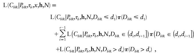 |
where d1<d2<…<dr are the ordered distances from x (in Mb) of the marker loci to the right of the disease locus. Given that recombination events occur at rate Nκ per Mb, per scaled unit of coalescent time,  , and
, and
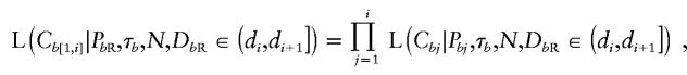
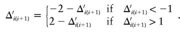
The marker haplotype between x and the NRE will be inherited, IBD, from the parental node to the offspring node, unless mutation occurs. The marker haplotype extending beyond the preserved region is assumed to have occurred as a result of recombination with a random chromosome from the population and thus occurs independently, according to the population proportions, h, in the same way as do the control chromosomes. Thus,
where Cb[i,j] is the offspring-node marker haplotype between loci i and j, inclusive. Given that marker-mutation events occur independently at rate Nμ per locus, per unit of coalescent time, it follows that
 |
where
 |
for each marker locus j⩽i.
Appendix C: Details of Metropolis Algorithm
Table C1.
Weights of Possible Changes to Current Parameter Set
| Change | Proposal | Parameter | Weighta |
| 1 | Location | x | 1 |
| 2 | Effective population size | N | 1 |
| 3 | Population allele proportion | p | m |
| 4 | Population LD parameter | Δ | m − 1 |
| 5 | Parental-status indicator | z | 2(nA − 1) |
| 6 | Ancestral haplotype | I | m(nA − 1) |
| 7 | Parental-node position | T and ϒ | 2(nA − 1) |
| 8 | Ordering of coalescent events | ϒ | nA − 2 |
| 9 | Waiting time | ϒ | nA − 1 |
| 10 | Missing information | u | |
| Overall | nA(6 + m) + m + u − 6 |
m = no. of diallelic marker loci; u = no. of untyped marker alleles, across sample of case and control chromosomes.
Each iteration of the Metropolis algorithm consists of a multistep proposal procedure. The current set of unknown model parameters and augmented data is denoted “ .” At each step, a new parameter set, 𝒮′, is proposed. To ensure reversibility, each proposal then consists of 1 of 10 possible changes to the parameter space, selected at random, according to predetermined weights (table C1). The new parameter set is substituted for the current parameter set, provided that
  for observed marker haplotypes
  , where α is a standard uniform random variable.
The possible changes to the current parameter set are summarized below, for a map of diallelic marker loci, with alleles coded “1” and “2” at each locus. For each proposed change, ε is a standard uniform random variable, and f is a constant that controls the maximum change in the parameter value.
Change 1: Propose a New Location for the Disease Locus
The proposed location is given by  . To ensure reversibility,
 |
where xL and xR denote the locations (in Mb) of the extremes of the candidate region.
Change 2: Propose a New Effective Population Size
The proposed population size is given by  . To ensure reversibility, N′=-N′ if the proposed population size is negative. A similar reflective boundary can be incorporated for an upper limit to effective population size, if necessary.
Change 3: Propose a New Population Marker-Allele Proportion
Select, at random, a marker, i, for the proposed proportion change. The proposed proportion of allele 1 at the selected marker is given by  . To ensure reversibility,
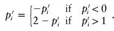 |
Change 4: Propose a New Population LD Parameter
Select, at random, a pair of adjacent markers, i and i+1, for the proposed parameter change. The proposed parameter is given by  . To ensure reversibility,
 |
Change 5: Propose a New Parental Status Indicator
Select, at random, a node, b, from the genealogical tree. The proposed parental state for the selected node is given by z′b=1-zb.
Change 6: Propose a New Allele for a Single Internal Node Marker Haplotype
Select at random, an internal node, b, from the tree. Select, at random, a marker, i, for the proposed change. The proposed allele, I′bi at the selected marker is given by I′bi=3-Ibi.
Change 7: Propose a New Position for the Parental Node of a Single Branch of the Tree
Figure C1.

Proposal of a new position for the parental node, Pb, on a selected branch of the genealogy, indicated by the dotted line (Change 6).
Figure C2.

Proposed new ordering for merging events between the most recent offspring node, O1b, and the parental node, Pb, of node b (i.e., Change 7).
Select, at random, a node, b, from the tree. The parent node of b is denoted “Pb”; the offspring node of the second branch descending from node Pb is denoted “Sb,” with “Ab” denoting the parent node of Pb. The current configuration is illustrated in figure C1. A new position for the parent node is chosen by selecting, at random, a branch from the tree. Equal weight is given to each branch, except for the following branches, which are all assigned weight zero:
the branch above node b;
the branch above node Pb;
the branch above node Sb;
any branch with the parental node below Pb ;
any branch with the offspring node above Pb.
By selecting a branch in this way, the time of the merging event corresponding to node Pb is preserved, with Ab and Sb replaced by A′b and S′b, the parent and offspring nodes of the selected branch.
Change 8: Propose a New Ordering for Merging Events between a Pair of Internal Nodes
Select, at random, an internal node, b, from the tree, a node corresponding to the merging event at time tb. We denote the parental node of b as “Pb,” occurring at time tPb. The two offspring nodes of b are denoted by “Ob1” and “Ob2,” with “tOb” denoting the time corresponding to the more ancient of these two merging events (fig. C2). The times corresponding to the merging events between tOb and tPb are denoted “ .” To choose a new ordering for the merging events, an internal node, S, is selected at random from those corresponding to the times t. The proposed ordering of waiting times is given by
  , where
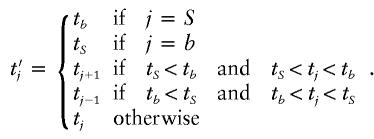 |
Change 9: Propose a New Waiting Time between Coalescent Events
Select an interval between adjacent coalescent events during which the tree has k distinct lineages. The proposed waiting time for the selected interval is given by  . To ensure reversibility, w′k=-wk if the proposed waiting time is negative.
Change 10: Propose a New Allele for Missing Marker Information
Select, at random, a chromosome, j, with missing marker information. Select, at random, a marker locus, i, from the missing information for chromosome j. The proposed allele is given by A′ji=3-Aji, for missing information from a case chromosome, and by U′ji=3-Uji, for missing information from a control chromosome.
Appendix D : Models for LD under a Star Genealogy
For the likelihood,  , in equation (7), we consider four models, which, on the basis of existing methods for fine-scale LD mapping, are denoted “COMP,” “STAR,” “PAIR,” and “LIU.”
COMP corresponds to a composite likelihood for independent markers, a likelihood for which
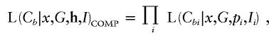 |
over all loci, i. The likelihood  can be calculated by noticing that Pb≡I for all leaf nodes and that Nτb≡G in equation (B1) and by following the probability arguments presented in Appendix B, under the assumption that only one marker locus is present to the right (or left) of the disease locus.
STAR and LIU correspond to a genuinely multipoint likelihood for complete marker haplotypes. This likelihood,
is calculated directly from the arguments presented in Appendix B, again by noticing that Pb≡I for all leaf nodes and that Nτb≡G in equation (B1).
PAIR corresponds to an approximate multipoint likelihood, which allows for pairwise correlation between case chromosomes and which is given by
The correction factor, c, depends only on the sample frequency of case chromosomes and is as derived by McPeek and Strahs (1999).
References
- Bertranpetit J, Calafell F (1996) Genetic and geographical variability in cystic fibrosis: evolutionary considerations. In: Weiss K (ed) Variation in the human genome. Wiley, Chichester, England, pp 97–114 [DOI] [PubMed] [Google Scholar]
- Clayton D (2000) Linkage disequilibrium mapping of disease susceptibility genes in human populations. Int Stat Rev 68:23–43 [Google Scholar]
- Collins A, Frezal J, Teague J, Morton NE (1996) A metric map of humans: 23,500 loci in 850 bands. Proc Natl Acad Sci USA 93:14771–14775 [DOI] [PMC free article] [PubMed] [Google Scholar]
- Collins A, Morton NE (1998) Mapping a disease locus by allelic association. Proc Natl Acad Sci USA 95:1741–1745 [DOI] [PMC free article] [PubMed] [Google Scholar]
- Donnelly P, Tavaré S (1995) Coalescents and genealogical structure under neutrality. Annu Rev Genet 29:401–421 [DOI] [PubMed] [Google Scholar]
- Graham J, Thompson EA (1998) Disequilibrium likelihoods for fine-scale mapping of a rare allele. Am J Hum Genet 63:1517–1530 [DOI] [PMC free article] [PubMed] [Google Scholar]
- Griffiths RC, Marjoram P (1996) Ancestral inference from samples of DNA sequences with recombination. J Comput Biol 3:479–502 [DOI] [PubMed] [Google Scholar]
- ——— (1997) An ancestral recombination graph. In: Donnelly P, Tavare S (eds) Progress in population genetics and human evolution. Springer-Verlag, New York, pp 257–270 [Google Scholar]
- Hartigan JA (1975) Clustering algorithms. Wiley, New York [Google Scholar]
- Hudson RR (1983) Properties of a neutral allele model with intragenic recombination. Theor Popul Biol 23:183–201 [DOI] [PubMed] [Google Scholar]
- ——— (1991) Gene genealogies and the coalescent process. In: Futuyma D, Antonovics J (eds) Oxford surveys in evolutionary biology. Oxford University Press, Oxford, pp 1–43 [Google Scholar]
- International Human Genome Sequence Consortium (2001) Initial sequencing and analysis of the human genome. Nature 409:860–921 [DOI] [PubMed] [Google Scholar]
- International SNP Map Working Group (2001) A map of the human genome sequence variation contain 1.42 million single nucleotide polymorphisms. Nature 409:928–933 [DOI] [PubMed] [Google Scholar]
- Kerem B, Rommens JM, Buchanan JA, Markiewicz D, Cox TK, Chakravarti A, Buchwald M, et al (1989) Identification of the cystic fibrosis gene: genetic analysis. Science 245:1073–1080 [DOI] [PubMed] [Google Scholar]
- Kingman JFC (1982) The coalescent. Stoch Proc Appl 13:235–248 [Google Scholar]
- Lam JC, Roeder K, Devlin B (2000) Haplotype fine mapping by evolutionary trees. Am J Hum Genet 66:659–673 [DOI] [PMC free article] [PubMed] [Google Scholar]
- Liu JS, Sabatti C, Teng J, Keats BJB, Risch N (2001) Bayesian analysis of haplotypes for linkage disequilibrium mapping. Genome Res 11:1716–1724 [DOI] [PMC free article] [PubMed] [Google Scholar]
- McCullagh P, Nelder J (1989) Generalized linear models, 2d ed. Chapman & Hall, London [Google Scholar]
- McPeek MS, Strahs A (1999) Assessment of linkage disequilibrium by the decay of haplotype sharing, with application to fine scale genetic mapping. Am J Hum Genet 65:858–875 [DOI] [PMC free article] [PubMed] [Google Scholar]
- Metropolis N, Rosenbluth AW, Rosenbluth MN, Teller AH, Teller E (1953) Equation of state calculations by fast computing machines. J Chem Phys 21:1087–1092 [Google Scholar]
- Moran P (1962) The statistical processes of evolutionary theory. Clarendon Press, Oxford [Google Scholar]
- Morral N, Bertranpetit J, Estivil X, Nunues V, Casals T, Gimenez J, Reis A, et al (1994) The origin of the major cystic fibrosis mutation (Delta-F508) in European populations. Nat Genet 7:169–175 [DOI] [PubMed] [Google Scholar]
- Morris AP, Whittaker JC, Balding DJ (2000) Bayesian mapping of disease loci using hidden Markov models. Am J Hum Genet 67:155–169 [DOI] [PMC free article] [PubMed] [Google Scholar]
- Nordborg M (2001) Coalescent theory. In: Balding DJ, Bishop M, Cannings C (eds) Handbook of statistical genetics. Wiley, Chichester, pp 179–212 [Google Scholar]
- Pennisi E (1998) A closer look at SNPs suggests difficulties. Science 281:1787–1789 [DOI] [PubMed] [Google Scholar]
- Rannala B, Reeve JP (2001) High-resolution multipoint linkage disequilibrium mapping in the context of a human genome sequence. Am J Hum Genet 69:159–178 [DOI] [PMC free article] [PubMed] [Google Scholar]
- Rannala B, Slatkin M (2000) Methods for multipoint disease mapping using linkage disequilibrium. Genet Epidemiol 19 Suppl 1:S71–S77 [DOI] [PubMed] [Google Scholar]
- Serre JL, Simon-Buoy B, Morret E, Jaume-Roig B, Balassopoulou A, Schwartz M, Taillander A (1990) Studies of RFLPs closely linked to the cystic-fibrosis locus throughout Europe lead to new considerations in population genetics. Hum Genet 84:449–454 [DOI] [PubMed] [Google Scholar]
- Slatkin M (1996) Gene genealogies within mutant allelic classes. Genetics 143:579–587 [DOI] [PMC free article] [PubMed] [Google Scholar]
- Slatkin M, Rannala B (1997) Estimating the age of alleles by use of intraallelic variability. Am J Hum Genet 60:447–458 [PMC free article] [PubMed] [Google Scholar]
- Terwilliger J (1995) A powerful likelihood method for the analysis of linkage disequilibrium between trait loci and one or more polymorphic marker loci. Am J Hum Genet 56:777–787 [PMC free article] [PubMed] [Google Scholar]
- Wedderburn RWM (1974) Quasi-likelihood functions, generalised models, and the Gauss-Newton method. Biometrika 61:439–447 [Google Scholar]
- Wiuf C, Donnelly P (1999) Conditional genealogies and the age of a neutral mutant. Theor Popul Biol 56:183–201 [DOI] [PubMed] [Google Scholar]
- Xiong M, Guo S-W (1997) Fine scale genetic mapping based on linkage disequilibrium: theory and applications. Am J Hum Genet 60:1513–1531 [DOI] [PMC free article] [PubMed] [Google Scholar]