

Abstract
Calcium puffs are local transient Ca2+ releases from internal Ca2+ stores such as the endoplasmic reticulum or the sarcoplasmic reticulum. Such release occurs through a cluster of inositol 1,4,5-trisphosphate receptors (IP3Rs). Based on the IP3R model (which is determined by fitting to stationary single-channel data) and nonstationary single-channel data, we construct a new IP3R model that includes time-dependent rates of mode switches. A point-source model of Ca2+ puffs is then constructed based on the new IP3R model and is solved by a hybrid Gillespie method with adaptive timing. Model results show that a relatively slow recovery of an IP3R from Ca2+ inhibition is necessary to reproduce most of the experimental outcomes, especially the nonexponential interpuff interval distributions. The number of receptors in a cluster could be severely underestimated when the recovery is sufficiently slow. Furthermore, we find that, as the number of IP3Rs increases, the average duration of puffs initially increases but then becomes saturated, whereas the average decay time keeps increasing linearly. This gives rise to the observed asymmetric puff shape.
Introduction
Intracellular Ca2+ signals, such as Ca2+ oscillations or waves, play a significant role in regulating many cellular activities, such as synaptic transmission, muscle contraction, saliva secretion, and cell fertilization and division (1–4). In many cell types, Ca2+ waves and oscillations are the result of Ca2+ liberation through clustered inositol 1,4,5-trisphosphate receptors (IP3Rs) located in the membrane of the endoplasmic reticulum (ER) or the sarcoplasmic reticulum (SR).
Ca2+ signaling is organized in a hierarchical manner (5). At the lowest level, stochastic release of Ca2+ through a single IP3R results in a small localized increase in cytoplasmic Ca2+ concentration ([Ca2+]), called a Ca2+ “blip.” Given the tightly clustered arrangement of IP3R, a Ca2+ blip can stimulate the release of additional Ca2+ through neighboring IP3Rs to cause release from a cluster of IP3Rs, giving a larger, but still localized, increase in [Ca2+], called a Ca2+ “puff.” At the highest level of organization, if enough puffs are generated, they can form a propagating wave of increased [Ca2+] across an entire cell.
Thus, a detailed study of Ca2+ puffs is necessary for understanding the dynamics of Ca2+ waves. Furthermore, an understanding of Ca2+ puffs relies on an accurate model of the IP3R, a model that can generate the correct statistical properties of the openings and closings of a single IP3R.
Until relatively recently, such a model was not available. Early IP3R models, such as the DeYoung–Keizer model (6) or the Atri model (7), reproduced such approximate statistics as the mean open time, or the steady-state open probability, but were based either on steady-state data alone or on single-channel data from lipid bilayers (8). In the years following those two initial models, many attempts were made to improve the IP3R models, including such features as time-dependent IP3R inactivation and multiple inactivated or inhibited states (9,10).
However, the field of IP3R modeling was dramatically changed by the appearance of new data, to our knowledge, of single-channel openings and closings from IP3R in vivo (11–13). For the first time, modelers were able to construct models of a single IP3R that could reproduce the correct statistical single-channel behavior in vivo (14–16). To our knowledge, these new data show that a single IP3R behaves in ways that cannot be reproduced by the older models. In particular, it appears that IP3Rs exist in different modes, each of which has a different open probability, and that activation of the IP3R is caused by a switch from one mode to another.
There are a number of studies of Ca2+ puffs already in the literature (17–27). Without exception, they are all based on older IP3R models, and thus fail to capture important aspects of the stationary behavior of a single IP3R. Hence, in light of recent data and models, it is necessary to reexamine the question of Ca2+ puff formation and how the hierarchy of Ca2+ signaling is constructed.
In particular, we wish to address some outstanding questions in the field. There are a number of such questions, but the ones we address here are as follows:
-
•
What is the mechanism of puff termination? Do the IP3Rs close due to inhibition by Ca2+, by stochastic attrition, or by some other inherent process?
-
•
What determines the distribution of interpuff intervals? Thurley et al. (28) performed a detailed analysis of interpuff intervals (IPI), that is, the waiting time between successive puffs, and found that some puff sites exhibit exponential IPI distributions but most sites have nonexponential distributions with a maximum at times larger than 0 s. This shows the stochastic occurrence of puffs is usually but not necessarily influenced by an inhibitory effect from the previous puffs, implying that the time constant of the inhibitory effect could be different for different puff sites. What kind of mechanism can generate both exponential and nonexponential IPI distributions? Is it possible that the mechanism is intrinsic to the IP3R instead of local depletion of the ER/SR, which has been shown to be unlikely by Ullah et al. (27)?
The most recent IP3R model is due to Siekmann et al. (16). The advantage of the Siekmann model is that its topological structure and transition rates are determined by Markov chain Monte Carlo (MCMC) fitting (29) directly to the stationary single-channel current traces instead of fitting only to statistical distributions. However, the Siekmann model fails to describe some earlier findings of transient behaviors shown in Mak et al. (13). To overcome this problem, we develop a new IP3R model with time-dependent state transitions by incorporating the recent nonstationary single-channel data from Mak et al. into the Siekmann model. Both of these data sets are measured from intact cells, and thus represent a significant improvement on the data used to construct previous models of the IP3R.
The Model
The Siekmann IP3R model
The Siekmann IP3R model is a six-state Markov model (Fig. 1) comprising two modes, park and drive, each of which has multiple closed and open states. When in park mode, the IP3R is mostly closed. When in drive mode, the IP3R is mostly open.
Figure 1.
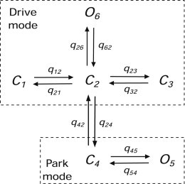
The structure of the Siekmann IP3R model. C represents closed state and O is open state; qs are transition rates connecting two adjacent states and indicating how fast an IP3R switches between the two states. The entire structure comprises two parts: One is the high-activity part or drive mode, containing three closed states , , , and one open state . The other is the low-activity part or park mode, which includes one closed state and one open state .
This model can be applied to two different isoforms of the IP3R, IP3R-1 and IP3R-2, by fitting the model to the corresponding single-channel data. Here, we focus on IP3R-1.
All the transition rates are constants except q24 and q42, and are given in Table S1 in the Supporting Material. In park mode, because q54 is ∼300 times greater than q45, the steady-state open probability of IP3R is almost zero. Conversely, in drive mode, the steady-state open probability is around 70% because of the fast transition pair of q26 and q62. The transitions q24 and q42 connecting the park and drive modes determine the open probability of the IP3R and are dependent on [Ca2+], [IP3], and [ATP] (12). For given [ATP] and [IP3], steady-state values of q24 and q42 are computed for different [Ca2+] (see symbols in Fig. S1). The stationary data were measured only at 0.1 mM and 5 mM [ATP]s (12,16). We use 0.1 mM [ATP] because it is closer to the [ATP] of 0.5 mM used for obtaining the dynamic data of Mak et al. (13). Investigating the effect of varying [ATP] needs more data and is beyond our current scope.
Incorporation of nonstationary data
Although, in theory, the openings and closing of the IP3R (in a stationary state) will contain enough information to characterize completely the rate constants in the Markov model, and thus determine the nonstationary behavior as well, in practice this is not the case here. Our stationary data, although sufficient to characterize the stationary behavior of the IP3R, do not contain enough information to also determine the transient behavior of the receptor (see Discussion).
We get around this difficulty by using additional data on transient responses and incorporate these data in a heuristic fashion rather than by the addition of states to the Markov model. Mak et al. (13) measured dynamic properties of the response of the IP3R to step changes in [Ca2+] or [IP3], and we modify the Siekmann model to incorporate these dynamic data. We accomplish this by assuming that q24 and q42 are controlled by gating variables that evolve on different timescales, which can be determined from the data of Mak et al. without changing their steady-state properties, which are determined by the data of Siekmann et al. (16).
Incorporation of these dynamic properties does not change the stationary behavior of the IP3R model. Hence, the fact that q24 and q42 are saturating functions of [Ca2+], which was an important feature of the Siekmann model, is preserved in our new model.
It turns out that these dynamic data are in fact crucial for the proper behavior of puffs in the model; the original Siekmann model does not provide an adequate description of puff behavior.
It is important to note that this modification of the Siekmann model is not based on rigorous MCMC fits to the data of Mak et al. (13). Instead, we choose the gating variables so as to give approximately correct distributions for the response to step changes of [Ca2+]. It is left for future work to do rigorous MCMC fits to both the steady-state and dynamic data simultaneously. Full details of the new model are given in the Supporting Material.
The transition rates q24 and q42 are given by
| (1) |
| (2) |
where , , , and are the gating variables that determine the values of q24 and q42; , , , and are either functions of [IP3] or constants, and are given in the Supporting Material.
We assume they obey the following differential equations:
| (3) |
where is the equilibrium and is the rate at which the equilibrium is approached. The are functions of [Ca2+] and are given by the following:
| (4) |
| (5) |
| (6) |
| (7) |
where the ns and ks are functions of [IP3] and are given in the Supporting Material. We emphasize that there are purely heuristic fits, with no biophysical basis. Hence, we have
| (8) |
| (9) |
which are used to fit to stationary single channel data from (16). Results are shown in Fig. S1 using a set of parameters given in the Supporting Material. For the case of 10 μM IP3, the MCMC method fails to work out convergent distributions of qs when [Ca2+] is between 1 and ∼50 μM, as the receptor is almost always in the drive mode so that very few mode switches can be detected (16). Therefore, for this range, we assume a saturated large q42 and a saturated small q24.
The rates , , and are constant, and are given in the Supporting Material. However, is not well determined by the data of Mak et al. (13). This could be due to the simplicity of the model wherein only two modes are considered. On the other hand, it is also possible that some unusual modes mislead the estimation of , as the experiments in Mak et al. use a wider range of [Ca2+] than that in Wagner and Yule (12) and Siekmann et al. (16), which constrain it to a physiological range. Because only two modes are unambiguously found by the MCMC methods (for the physiological range of [Ca2+]), we will not add any more states or modes to the Siekmann model. Instead, we shall estimate from puff data in Smith and Parker (30), in which it is found that most puffs exhibit fast increases from baseline to the peak, with sharp peaks instead of plateaus. This reveals that IP3Rs are inhibited by high [Ca2+] very quickly and are hard to reopen immediately, telling us that is relatively small for low [Ca2+] but relatively large for high [Ca2+]. Therefore, we model by the following:
| (10) |
This is merely a heuristic way of modeling a stepwise rate that is low at low [Ca2+] and high at high [Ca2+]. Because we have no information about the exact concentration at which this transition occurs, we arbitrarily assume it to occur at 20 μM. In addition, we choose s−1 to represent fast inhibition by Ca2+. Because dominates the recovery rate of an IP3R inhibited by Ca2+, and in turn has a significant effect on IPIs, we use it as a parameter instead of a constant to investigate how it alters the IPI distributions.
Modeling Ca2+ puffs using two different Ca2+ concentrations
Rüdiger et al. (25) used two different [Ca2+]s to model puffs: a high constant [Ca2+] at each open channel mouth and a low average [Ca2+] for all the closed channels. This method ignores Ca2+ diffusion and the spatial distribution of the IP3Rs, and therefore dramatically increases the computational efficiency. Here, we apply the same idea to build our puff model. A detailed justification of this assumption is given in Rüdiger et al. (24,25) and Nguyen et al. (26).
Let c be the average low [Ca2+] and let be the [Ca2+] at the IP3R mouth. Before formulating the model, some assumptions need to be made:
-
•
Ca2+ fluxes through the plasma membrane do not influence Ca2+ puffs.
-
•
The rate of Ca2+ release through single IP3R is a constant. In other words, there is sufficiently high [Ca2+] in the ER/SR to keep a nearly constant flux. Although local depletion of the ER/SR is possible for some types of cells, it should not be the case for puffs observed in Dickinson et al. (18) and Smith and Parker (30), as [Ca2+] can be kept at an elevated level when the channel is sustainedly open and the stepwise increments of those puffs do not get progressively smaller.
-
•
The endogenous fast buffers are immobile, unsaturated, and in quasi-steady state. We have shown that relaxation of these assumptions does not qualitatively change the puff statistics, especially in some important aspects such as the IPI distribution and puff duration distribution (results not shown).
-
•
The limited effect of endogenous slow buffers on puff dynamics is ignored. We also ignore the effect of EGTA, a slow buffer used in the experiments to isolate different puff sites by decreasing the effective Ca2+ diffusivity (30).
With these assumptions, the differential equations governing the dynamics of c are
| (11) |
| (12) |
is the Ca2+ flux contributing to the increase of c. represents the flux (mainly via diffusion and sarcoplasmic/endoplasmic reticulum Ca2+-ATPase ) removing Ca2+ from the puff site and is modeled by , where and are constants. In addition, a linear model of with an appropriate conductance can also be used (result not shown). is Ca2+ leakage from the ER/SR, and is necessary for establishing a stable resting cytosolic [Ca2+]. A Ca2+ dye (fluo-4) is added to the model, as all the experimental statistical analyses are done by using the fluorescence ratio instead of [Ca2+]. and bfluo4 represent the total fluo-4 concentration and Ca2+-bound fluo-4 concentration, respectively.
denotes the number of open IP3Rs and satisfies (total number of functional IP3Rs). It is computed by direct counting of the IP3R states, and then is used to calculate c by integrating Eq. 11. To determine the state of each IP3R, we use , which is modeled by
| (13) |
where δ indicates whether the IP3R is open (δ = 1) or closed (δ = 0). is the constant high [Ca2+] at the receptor mouth. δ is a stochastic variable that depends on via the stochastic solution of the IP3R model. All the parameter values are given in Table S2.
Numerical methods
We solve Eqs. 11 and 12 in a deterministic way but apply a stochastic solver to the IP3R dynamics. Eqs. 11 and 12 are solved by the fourth-order Runge–Kutta method. To solve the stochastic IP3R model, a hybrid Gillespie method with adaptive timing is used to take into account the Ca2+ dependencies of transitions q24 and q42 (31). We choose a maximum time step size of 10−4 s to guarantee the accuracy. In addition, the four differential equations in Eq. 3 are solved by the fourth-order Runge–Kutta method as well. All the numerical results are obtained using the software MATLAB (The MathWorks, Natick, MA).
Results
We focus on investigating how the puff statistics are influenced by the following three parameters:
-
•
[IP3] (p),
-
•
recovery rate of an IP3R from Ca2+ inhibition , and
-
•
the number of IP3Rs at a puff site
as they are found experimentally to be important to the puff dynamics.
Calcium puffs
Fig. 2 shows an example of simulated puff traces. represents the ratio of to its resting value. We can see that a large puff usually needs openings of sufficiently many receptors. To investigate how puffs are initiated and terminated, we rescale the puff amplitude and plot it, together with and , in Fig. 3 ( and are calculated by averaging over all the IP3Rs). In the lower panel of Fig. 3, we can see a “trigger” event at the beginning of the puff, which leads to a fast upstroke of the activation variable , which then further increases the open probability of IP3Rs. This trigger event has been found experimentally (32). Termination of Ca2+ release is achieved when gets close to zero. During the falling phase, open IP3Rs close randomly and independently with an average open time determined by and (results not shown), as they are hard to open again when is very small. The slow recovery of , which is due to the small value of used, influences the average IPI and the next puff amplitude. This is investigated in the Supporting Material.
Figure 2.
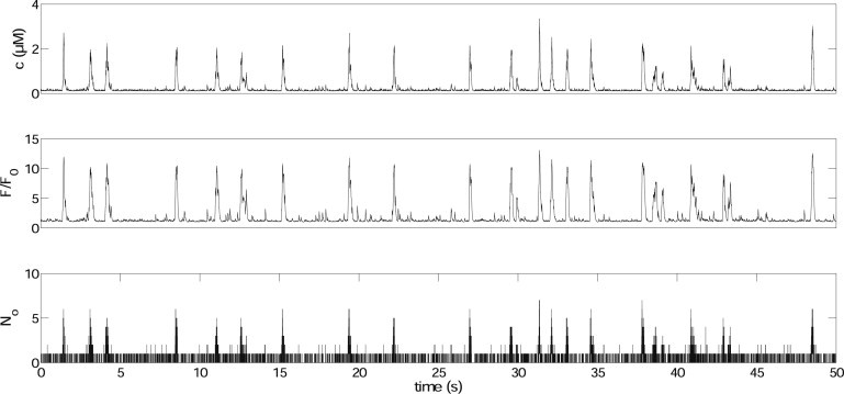
An example of simulation results of calcium puff traces. The top panel shows an example of the [Ca2+] trace (variable c in Eq. 11). represents the ratio of to its resting value. We set , μM, and s−1.
Figure 3.
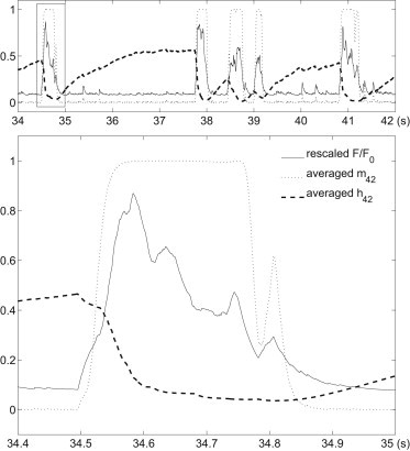
A close-up of some puffs in Fig. 2. The lower panel is an enlargement of the rectangular portion of the upper panel. The ratio (solid curve) is rescaled into the interval [0,1] for ease of comparison with and .
We can see in Fig. 2 that there are many small blips and other noise in the puff trace. To eliminate this noise, we choose puffs with amplitude larger than 3, that is, . The choice of this value is based on the simulated blip amplitude distribution and the mean blip amplitude of 1.6. Details are given in the Supporting Material.
Dependence of IPI distribution on ah42
Experimental IPI distributions exhibit two different shapes, exponential and nonexponential (28). The former indicates that there is no (or very little) refractoriness during the IPIs, whereas the latter implies an apparent refractory phase after each puff. A formula that gives excellent fits to experimental IPI distributions has been proposed by Thurley et al. (28) as follows:
| (14) |
where λ is the puff rate, a measure of the typical IPI (similar to average puff frequency), and ξ is the recovery rate. This formula is derived based on the assumption that there is a refractory period after a puff. If , Eq. 14 can be reduced to a simple exponential distribution,
| (15) |
Refractoriness of simulated puffs comes from the slow recovery of from inhibition by Ca2+. This implies that varying could change the duration of refractoriness and, in turn, change the shape of IPI distribution. This is confirmed by Fig. 4, which shows that increasing from 0.1 s−1 to 5 s−1 leads to a change of the simulated IPI distribution from nonexponential to exponential. The details of the fits shown in Fig. 4 are given in Fig. S5, in which we can see that values for λ vary from 0.1 s−1 to 0.5 s−1 and values for ξ vary from 0.5 s−1 to 2.2 s−1. These results are quantitatively consistent with the experimental ranges of λ and ξ found in SH-SY5Y cells, that from 0.18 s−1 to 0.5 s−1 for λ and from 0.4 s−1 to 4 s−1 for ξ. Moreover, it is also found that in HEK 293 cells, values for λ and ξ are in the ranges from 0.5 s−1 to 3 s−1 and from 1 s−1 to 90 s−1, respectively (5,28).
Figure 4.
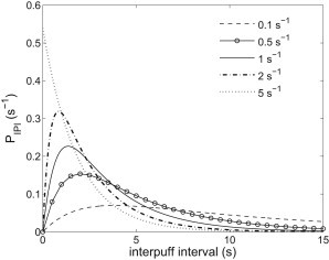
Various simulated IPI distributions for different . We set , μM. The values of are indicated in the legend. For a given , we choose appropriate values of λ and ξ to fit to the corresponding simulated IPI distributions using Eq. 14 or Eq. 15. Then the values of λ and ξ are used to plot these curves in the figure. Fitting details and results are given in the Supporting Material.
Coefficient of variation is independent of [IP3]
For a puff site, the IPI standard deviation has been shown to be linearly related to the IPI mean, regardless of [IP3] (28). A qualitatively consistent result occurs in the model (Fig. 5), in which we plot the IPI standard deviation against the IPI mean. The coefficient of variation (CV) is defined as the ratio of the standard deviation to the mean of IPIs. When , the IPI is a homogeneous Poisson process (the dashed line in Fig. 5), whereas when , the IPI is a constant, giving an entirely periodic series of puffs. Other values of the CV between 0 and 1 indicate an inhomogeneous Poisson process with refractoriness. In our model, the CV is 0.79, which is in reasonable agreement with experimental values (that vary from 0.42 to 0.94 for different types of cells (28)). Therefore, the model result not only confirms the nonexponential IPI distribution in Fig. 4, but also implies that a relatively slow recovery of IP3R from Ca2+ inhibition could be a key mechanism of modulating IPI. We also find that changing the value of can vary the CV between 0.65 and 0.95. The relation is not very clear, as can also change some other statistics, such as average IPI and puff amplitude, which could in turn influence the CV. This is left for future work.
Figure 5.
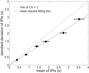
Relation of standard deviation and mean of IPI is linear and independent of [IP3]. Six [IP3]s, 0.05, 0.1, 0.15, 0.2, 0.3, and 0.5 (μM), are used to generate the six points (from right to left), respectively. The points are expressed as mean ± SE and are fit by a solid line with slope of 0.79 compared with the dashed line of CV = 1. We set and s−1.
Dependence of IPI on the number of IP3Rs at a puff site
It has been found experimentally and by model simulations that the IPI mean is a hyperbolic function of , the number of IP3Rs at a puff site (18). This implies a linear relationship between the IPI mean and . This relationship is reproduced by our model (Fig. 6). Moreover, we find that varying [IP3] changes the slope of the linear fit, but has little effect on the linearity of the relationship. We explain this as follows. If is the probability per unit time for opening of a single channel at baseline, then is the probability per unit time for opening of one of the channels. Hence, the average IPI is proportional to . Because a saturated low calcium sensitivity near the baseline of 0.1 μM is assumed in the IP3R model (Fig. S1), is nearly a constant for [Ca2+] close to baseline, which implies that the average IPI is simply proportional to .
Figure 6.
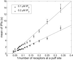
Linear relationship between mean of IPIs and , the reciprocal of the number of IP3R at a puff site. is chosen to be 3 ∼ 15, 20, and 25. For each value of , means of IPIs for two different [IP3]s, 0.1 μM and 0.2 μM, are computed and expressed as mean ± SE. For each [IP3], a least-square linear fitting is performed and plotted using a solid line. We set s−1.
For small numbers of IP3R, the model (Fig. 6) has longer IPIs than does the data (see Fig. 4E in Dickinson et al. (18)). There could be two reasons for this. One is that the applied [IP3] is different. The other is that the cluster size estimated in the experiments is severely underestimated because of a very slow recovery rate (Fig. S6). For either of these reasons, the discrepancy can be easily fixed by changing model parameters.
The relationship between IPI and latency
Puff latency is defined to be the waiting time from addition of to the occurrence of the first puff (18). The biggest difference between IPI and latency is that the former could contain some inhibition effect from the preceding puff, whereas the latter definitely does not contain such an effect. Similar to Fig. 4D in Dickinson et al. (18), we plot the IPI mean and latency for different (Fig. 7), and find that they are linearly related with a slope of ∼1.2 and a positive IPI-axis intercept of ∼0.35 s (which are close to the slope of 1.1 and intercept of 0.35 s found experimentally). The intercept gives the average effective time of the inhibitory effect of the preceding puffs on the next IPI. The quantitative agreement between model results and experimental data shows that the preceding puff has a clear inhibitory effect on the occurrence of the next puff. Moreover, by investigating the dependence of puff amplitude on the preceding IPI (see the Supporting Material), we find that the inhibitory effect is time-dependent, which is also found experimentally (33).
Figure 7.
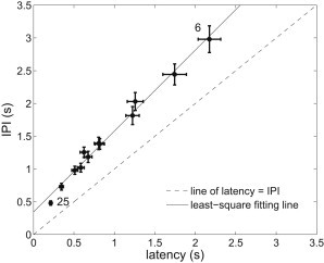
IPI is linearly dependent on puff latency. is chosen to be 6 ∼ 15, 20, and 25. Only are the points of 6 and 25 IP3R channels labeled. Small values of , such as 3 ∼ 5, are excluded in the figure for a better view because they will not change the linearity but significantly increase the scales of axes. Results are plotted as mean ± SE and fit by the solid line. The dashed line indicates where IPI is equal to latency. We set μM and s−1.
Dependence of puff amplitude on number of IP3Rs at a puff site
Fig. 8 shows the dependence of average puff amplitude and the largest puff amplitude (both normalized to mean blip amplitude) on the number of IP3Rs at a puff site . Both amplitudes increase as increases. The average amplitude is linearly related to for . However, when , it behaves like the square root of . Because our model assumes that the rate of Ca2+ release through a single channel is a constant, we rule out ER/SR depletion as a reason for the nonlinearity. To check whether it is due to the nonlinear relation between Ca2+ and buffer, we plot the puff [Ca2+] amplitude instead of the Ca2+-bound buffer (Fig. S9) and find that the average puff [Ca2+] amplitude is linearly dependent on . This result shows that the nonlinear relation of puff amplitude and in Fig. 8 is caused by using the Ca2+ buffer to indicate puff amplitude. Although no severe buffer saturation is observed, the nonlinearity of the buffering indicator inevitably affects the observed results, as the height of [Ca2+] for large puffs can easily become higher than the dissociation constant of fluo-4 of 2 μM.
Figure 8.
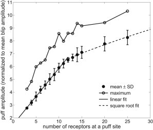
Dependence of average puff amplitude and the largest puff amplitude on the number of IP3R at a puff site. Amplitudes are normalized to mean blip amplitude, 1.6. A linear fit is performed for , whereas a square root function gives an excellent fit to the points of . The average puff amplitude is expressed as mean ± SD. We set μM and s−1.
Another important relationship obtained by combining Fig. 8 and Fig. S9 is that the average puff amplitude is nonlinearly related to the average maximum Ca2+ current in a similar way, as maximum Ca2+ current can be roughly assumed to be proportional to puff [Ca2+] amplitude.
Dependence of puff duration on the number of IP3Rs at a puff site
Experimental puffs usually exhibit a rapid increase to the peak but a relatively slow return to baseline (30). This property is also seen in the model (Fig. 9). As increases, the average rise time gets saturated to ∼130 ms, whereas the average decay time keeps increasing linearly. This gives rise to an asymmetric puff shape for larger . However, for smaller , the two times are close to each other, which indicates that small puffs are relatively symmetric. The linear dependence of average decay time on the number of receptors is primarily a consequence of the fact that the IP3Rs close randomly and independently (30). The saturation of rise time could be caused by two reasons. One is the puff amplitude saturation observed in Fig. 8. The other is that sufficient high average [Ca2+] (c) during Ca2+ release through a few initially activated channels prevents other closed channels from opening. The former seems not to be very convincing, as the amplitude saturation occurs when , whereas the rise time saturation takes place when is only ∼8. Hence, the latter is preferred to be a major reason for the phenomenon.
Figure 9.
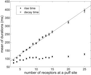
Puff rise time and decay time are differently dependent on the number of IP3R. Results are plotted as mean ± SE. Points of decay time are fit linearly (solid line). We set μM and s−1.
Discussion
Ca2+ puffs are local transient Ca2+ release events from internal Ca2+ stores such as the ER or the SR through a cluster of open IP3Rs. For a better understanding of the mechanisms underlying this physiological phenomenon, we first construct a new mathematical model of the IP3R, based mostly on the Siekmann IP3R model (16), but also incorporating the time-dependent data of Mak et al. (13). By construction, we know that our new model fits the stationary data equally as well as the original Siekmann model. It merely has additional time-dependencies to allow for the correct transient behavior. We then show how our model qualitatively and quantitatively reproduces experimentally observed puff statistics. The most important feature of our model is that the IP3R can recover from inhibition by Ca2+ only on a relatively slow timescale. This timescale cannot be identified from the stationary data of Siekmann et al., but depends on the nonstationary data of Mak et al.
This is an important point worth emphasizing. We know (theoretically) that a sufficiently long experimental trace will contain information about the behavior of the IP3R on both long and short timescales, and thus will be sufficient to determine both steady-state and transient behavior. However, the reality is more complex. In practice, such long traces are not obtainable, and, even if they were, fitting to the data would require unrealistically large amounts of computer time because of the rarity of the slow transitions. Thus, fitting the stationary data alone will determine only some of the important receptor properties.
Interestingly, it turns out that the slow processes are vital for controlling the inhibition of the IP3R; thus, puffs do not occur often enough (in the stationary state) to be characterized by stationary data using our methods.
There are thus two options. The first option would be to incorporate nonstationary data (i.e., the responses to steps of [IP3] and/or [Ca2+]) into the full fitting process, and thereby construct an extended Markov model, with more than the present 6 states. One would then continue to include additional states until the MCMC fits to the data indicated that additional states were unnecessary or that the additional rate constants could not be unambiguously determined. Ullah et al. (15) took an approach similar to this (although their method of fitting to data is different from that of Siekmann et al. (16)), constructing a Markov model with 12 states. However, the model of Ullah et al. cannot successfully reproduce calcium puffs. This failure is primarily due to lack of an effective transition from the inactivated state to the resting state, without which transition the receptors lose the excitability that is crucial for generating repetitive puffs and waves.
The second option, which we took, is to construct a hybrid model, partaking both of the nature of Markov models (such as the De Young–Keizer model) and of heuristic models (such as the Atri model). This has the advantage that we need not introduce any additional states into the Markov model, but it has the disadvantage that the time-dependent transitions we introduce have no biophysical basis. However, we have lost less than one might think. It is highly unlikely that an actual IP3R exists in exactly 6 states (or even 60 states), with well-defined transitions between them. In general, it is thus more accurate to interpret Markov models as useful descriptions rather than as exact biophysical reality, in which case a hybrid Markov/heuristic model is just as useful.
Finally, we note that although the new model still does not reproduce every aspect of the nonstationary data (i.e., it does not reproduce multimodal waiting time distributions), it still captures the most important features of the dynamic data by reproducing the most dominant modes of those distributions.
The hybrid nature of our model raises some interesting questions. Which part of our model is primarily responsible for the puff dynamics? We know that the Markov model, with time-independent rate constants, does not provide an adequate description of puff dynamics. This is why we introduced the heuristic time dependencies in the first place. However, can the Markov model skeleton be replaced by a simpler model (most likely with the incorrect stationary behavior) as long as the heuristic time dependencies are retained?
We can answer only some of these questions. For example, one implication of Fig. 4 is that the original Siekmann IP3R model (that fits only to stationary single-channel data) cannot be used to reproduce the nonexponential IPI distributions. In Eq. 3, if λG is sufficiently larger than the average change velocity of c, G can be reasonably assumed to follow its equilibrium at any time. Thus, , , and evolve nearly as their equilibria, whereas evolves on a much slower timescale indicated by a small value of . As increases, the evolution of becomes closer to its equilibrium. However, a consequence of this change is that the feature of the nonexponential IPI distribution gradually disappears and becomes closer to an exponential distribution. This implies that the inhomogeneity of the occurrence of puffs is primarily caused by the slow recovery of . Therefore, assuming that the IP3R can instantaneously follow the steady state cannot reproduce results that fully explain the experimental data, which confirms the necessity of introducing a relatively slow recovery rate .
However, we do not yet know the simplest possible version of our model that can generate correct IPI distributions or other puff statistics. Preliminary results indicate that the modal nature of the IP3R plays little role in the dynamics of puffs and can thus reasonably be ignored in studies of periodic Ca2+ waves. In this case, the simplest Markov scheme is just a two-state open/closed model, with time-dependent transitions. However, a complete study of this question is well beyond the scope of this article and is left for future work.
A major assumption in our model is that is heuristically modeled by Eq. 10 wherein an important parameter, , is introduced to indicate the recovery rate of a single IP3R from inhibition by Ca2+. This assumption is based on the appearance and statistics of observed puffs, rather than on nonstationary single-channel data in Mak et al. (13), because a relatively long (∼2.4 s) recovery time given by the data in Mak et al. cannot be achieved otherwise by our model. The failure is mainly due to the saturation of curves for high [Ca2+], as seen in Fig. S1b. To resolve the problem, we need to consider two aspects. One is whether the stationary single-channel data support a smaller value of for 300 μM [Ca2+]. The other is whether [Ca2+] at the channel mouth during Ca2+ release can reach 300 μM. The former needs more stationary data, whereas the latter is still not clearly known. If [Ca2+] can reach 300 μM, then we need to modify the existing model, especially the values of for high [Ca2+]. But if [Ca2+] can only reach ∼100 μM, the dynamic data for 300 μM are not sufficient to reveal the actual recovery rate. Because of this uncertainty, we use Eq. 10 as an alternative way of modeling the slow recovery process.
Our new model is, to our knowledge, the first to reproduce, simultaneously, the correct statistics of IP3R opening and closing, as well as the correct puff statistics. Although most of the model results, like Figs. 5–9, could qualitatively be reproduced by some older models (18,20–27), none of these older models demonstrate the correct IP3R statistical behavior. In addition, our model demonstrates that slow recovery of an IP3R from Ca2+ inhibition is a crucial feature for Ca2+ puffs, and shows also how the IPI distribution is affected by the recovery rate (Fig. 4). We find that various IPI distributions (either exponential or nonexponential, both of which are seen experimentally (28)) obtained by varying the recovery rate, , reveal that different puff sites could exhibit different average recovery rates. In addition, we also find that puff amplitude initially increases but then becomes saturated as increases (Fig. S6). This suggests that the number of IP3Rs at a puff site could be severely underestimated if the average recovery process is sufficiently slow.
We investigate the relation of puff amplitude and IPI in the Supporting Material (Fig. S8), based on which we find that a saturation in Fig. S8 occurs at about . This could be a way of estimating from experimental data. In addition, we find the following IPI seems to be independent on the preceding puff amplitude by looking at the scatterplot similar to Fig. S7 (results not shown). This could be explained by Fig. 3, in which we can see that the inactivation variable will quickly drop to be very close to zero during a puff regardless of the puff amplitude. Therefore, the inhibitory effect from preceding puffs with various amplitudes on the following IPIs is nearly identical.
Puff amplitude has been reported to be nonlinearly related to the maximum Ca2+ current such that, as maximum Ca2+ current increases, puff amplitude initially increases linearly but then becomes proportional to the square root of maximum Ca2+ current (19,34,35). Our model gives the same result. Thurley et al. (19) suggested that the nonlinearity is due to local Ca2+ depletion in the ER/SR. However, this conclusion was challenged by Solovey et al. (35), who showed that this nonlinearity could be generated by a mean field model or by using a stochastic model with a constant single-channel Ca2+ flux. They also concluded that the nonlinear relation was due to the dynamics of the Ca2+-bound dye. By comparing the nonlinear relation between average puff amplitude and the number of IP3Rs (Fig. 8) and the linear relation between average puff [Ca2+] amplitude and the number of IP3Rs (Fig. S9), our model supports the conclusion of Solovey et al. by showing that nonlinearity arises from the nonlinear relationship between [Ca2+] and Ca2+-bound buffer concentration, even when Ca2+-bound buffer is not saturated.
Ca2+ oscillations and waves usually exhibit a relatively long decay time and periods ranging from a few seconds to a few minutes. The mechanisms underlying long-period waves remain unclear; this is perhaps the most important unsolved problem in the theoretical study of Ca2+ waves. One can obtain stochastically generated long-period waves in models that do not have the correct puff statistics, but there is as yet no model that has the correct IP3R statistics and the correct puff statistics and can generate long-period waves. Our own preliminary computations indicate that our new model can generate short-period waves (around a few seconds) but not waves of longer period. However, we leave a detailed study of this question for a future article.
Supporting Material
References
- 1.Berridge M.J. Elementary and global aspects of calcium signalling. J. Physiol. 1997;499:291–306. doi: 10.1113/jphysiol.1997.sp021927. [DOI] [PMC free article] [PubMed] [Google Scholar]
- 2.Berridge M.J., Lipp P., Bootman M.D. The versatility and universality of calcium signalling. Nat. Rev. Mol. Cell Biol. 2000;1:11–21. doi: 10.1038/35036035. [DOI] [PubMed] [Google Scholar]
- 3.Keener J.P., Sneyd J. Springer-Verlag; New York: 2009. Mathematical Physiology. [Google Scholar]
- 4.Bergner A., Sanderson M.J. Acetylcholine-induced calcium signaling and contraction of airway smooth muscle cells in lung slices. J. Gen. Physiol. 2002;119:187–198. doi: 10.1085/jgp.119.2.187. [DOI] [PMC free article] [PubMed] [Google Scholar]
- 5.Thurley K., Skupin A., Falcke M. Fundamental properties of Ca2+ signals. Biochim. Biophys. Acta. 2012;1820:1185–1194. doi: 10.1016/j.bbagen.2011.10.007. [DOI] [PubMed] [Google Scholar]
- 6.De Young G.W., Keizer J. A single-pool inositol 1,4,5-trisphosphate-receptor-based model for agonist-stimulated oscillations in Ca2+ concentration. Proc. Natl. Acad. Sci. USA. 1992;89:9895–9899. doi: 10.1073/pnas.89.20.9895. [DOI] [PMC free article] [PubMed] [Google Scholar]
- 7.Atri A., Amundson J., Sneyd J. A single-pool model for intracellular calcium oscillations and waves in the Xenopus laevis oocyte. Biophys. J. 1993;65:1727–1739. doi: 10.1016/S0006-3495(93)81191-3. [DOI] [PMC free article] [PubMed] [Google Scholar]
- 8.Bezprozvanny I., Watras J., Ehrlich B.E. Bell-shaped calcium-response curves of ins(1,4,5)P3- and calcium-gated channels from endoplasmic reticulum of cerebellum. Nature. 1991;351:751–754. doi: 10.1038/351751a0. [DOI] [PubMed] [Google Scholar]
- 9.Sneyd J., Falcke M., Fox C. A comparison of three models of the inositol trisphosphate receptor. Prog. Biophys. Mol. Biol. 2004;85:121–140. doi: 10.1016/j.pbiomolbio.2004.01.013. [DOI] [PubMed] [Google Scholar]
- 10.Sneyd J., Falcke M. Models of the inositol trisphosphate receptor. Prog. Biophys. Mol. Biol. 2005;89:207–245. doi: 10.1016/j.pbiomolbio.2004.11.001. [DOI] [PubMed] [Google Scholar]
- 11.Foskett J.K., White C., Mak D.O.D. Inositol trisphosphate receptor Ca2+ release channels. Physiol. Rev. 2007;87:593–658. doi: 10.1152/physrev.00035.2006. [DOI] [PMC free article] [PubMed] [Google Scholar]
- 12.Wagner, L. E., and D. I. Yule. 2011. Differential regulation of the inositol 1,4,5-trisphosphate receptor type-1 and -2 single channel properties by InsP3, Ca2+ and ATP. J. Physiol.http://jp.physoc.org/content/early/2012/04/30/jphysiol.2012.228320. Abstract. [DOI] [PMC free article] [PubMed]
- 13.Mak D.O.D., Pearson J.E., Foskett J.K. Rapid ligand-regulated gating kinetics of single inositol 1,4,5-trisphosphate receptor Ca2+ release channels. EMBO Rep. 2007;8:1044–1051. doi: 10.1038/sj.embor.7401087. [DOI] [PMC free article] [PubMed] [Google Scholar]
- 14.Gin E., Falcke M., Sneyd J. A kinetic model of the inositol trisphosphate receptor based on single-channel data. Biophys. J. 2009;96:4053–4062. doi: 10.1016/j.bpj.2008.12.3964. [DOI] [PMC free article] [PubMed] [Google Scholar]
- 15.Ullah G., Mak D.O.D., Pearson J.E. A data-driven model of a modal gated ion channel: the inositol 1,4,5-trisphosphate receptor in insect Sf9 cells. J. Gen. Physiol. 2012;140:159–173. doi: 10.1085/jgp.201110753. [DOI] [PMC free article] [PubMed] [Google Scholar]
- 16.Siekmann I., Wagner L.E., 2nd, Sneyd J. A kinetic model for type I and II IP3R accounting for mode changes. Biophys. J. 2012;103:658–668. doi: 10.1016/j.bpj.2012.07.016. [DOI] [PMC free article] [PubMed] [Google Scholar]
- 17.Shuai J., Rose H.J., Parker I. The number and spatial distribution of IP3 receptors underlying calcium puffs in Xenopus oocytes. Biophys. J. 2006;91:4033–4044. doi: 10.1529/biophysj.106.088880. [DOI] [PMC free article] [PubMed] [Google Scholar]
- 18.Dickinson G.D., Swaminathan D., Parker I. The probability of triggering calcium puffs is linearly related to the number of inositol trisphosphate receptors in a cluster. Biophys. J. 2012;102:1826–1836. doi: 10.1016/j.bpj.2012.03.029. [DOI] [PMC free article] [PubMed] [Google Scholar]
- 19.Thul R., Falcke M. Release currents of IP(3) receptor channel clusters and concentration profiles. Biophys. J. 2004;86:2660–2673. doi: 10.1016/S0006-3495(04)74322-2. [DOI] [PMC free article] [PubMed] [Google Scholar]
- 20.Swaminathan D., Ullah G., Jung P. A simple sequential-binding model for calcium puffs. Chaos. 2009;19:037109. doi: 10.1063/1.3152227. [DOI] [PMC free article] [PubMed] [Google Scholar]
- 21.Shuai J., Pearson J.E., Parker I. A kinetic model of single and clustered IP3 receptors in the absence of Ca2+ feedback. Biophys. J. 2007;93:1151–1162. doi: 10.1529/biophysj.107.108795. [DOI] [PMC free article] [PubMed] [Google Scholar]
- 22.Solovey G., Fraiman D., Ponce Dawson S. Simplified model of cytosolic Ca2+ dynamics in the presence of one or several clusters of Ca2+-release channels. Phys. Rev. E Stat. Nonlin. Soft Matter Phys. 2008;78:041915. doi: 10.1103/PhysRevE.78.041915. [DOI] [PubMed] [Google Scholar]
- 23.Higgins E.R., Schmidle H., Falcke M. Waiting time distributions for clusters of IP3 receptors. J. Theor. Biol. 2009;259:338–349. doi: 10.1016/j.jtbi.2009.03.018. [DOI] [PubMed] [Google Scholar]
- 24.Rüdiger S., Shuai J.W., Sokolov I.M. Law of mass action, detailed balance, and the modeling of calcium puffs. Phys. Rev. Lett. 2010;105:048103. doi: 10.1103/PhysRevLett.105.048103. [DOI] [PubMed] [Google Scholar]
- 25.Rüdiger S., Jung P., Shuai J.W. Termination of Ca²+ release for clustered IP3R channels. PLoS Comput. Biol. 2012;8:e1002485. doi: 10.1371/journal.pcbi.1002485. [DOI] [PMC free article] [PubMed] [Google Scholar]
- 26.Nguyen V., Mathias R., Smith G.D. A stochastic automata network descriptor for Markov chain models of instantaneously coupled intracellular Ca2+ channels. Bull. Math. Biol. 2005;67:393–432. doi: 10.1016/j.bulm.2004.08.010. [DOI] [PubMed] [Google Scholar]
- 27.Ullah G., Parker I., Pearson J.E. Multi-scale data-driven modeling and observation of calcium puffs. Cell Calcium. 2012;52:152–160. doi: 10.1016/j.ceca.2012.04.018. [DOI] [PMC free article] [PubMed] [Google Scholar]
- 28.Thurley K., Smith I.F., Falcke M. Timescales of IP(3)-evoked Ca(2+) spikes emerge from Ca(2+) puffs only at the cellular level. Biophys. J. 2011;101:2638–2644. doi: 10.1016/j.bpj.2011.10.030. [DOI] [PMC free article] [PubMed] [Google Scholar]
- 29.Siekmann I., Wagner L.E., 2nd, Sneyd J. MCMC estimation of Markov models for ion channels. Biophys. J. 2011;100:1919–1929. doi: 10.1016/j.bpj.2011.02.059. [DOI] [PMC free article] [PubMed] [Google Scholar]
- 30.Smith I.F., Parker I. Imaging the quantal substructure of single IP3R channel activity during Ca2+ puffs in intact mammalian cells. Proc. Natl. Acad. Sci. USA. 2009;106:6404–6409. doi: 10.1073/pnas.0810799106. [DOI] [PMC free article] [PubMed] [Google Scholar]
- 31.Rüdiger S., Shuai J.W., Falcke M. Hybrid stochastic and deterministic simulations of calcium blips. Biophys. J. 2007;93:1847–1857. doi: 10.1529/biophysj.106.099879. [DOI] [PMC free article] [PubMed] [Google Scholar]
- 32.Rose H.J., Dargan S., Parker I. “Trigger” events precede calcium puffs in Xenopus oocytes. Biophys. J. 2006;91:4024–4032. doi: 10.1529/biophysj.106.088872. [DOI] [PMC free article] [PubMed] [Google Scholar]
- 33.Fraiman D., Pando B., Dawson S.P. Analysis of puff dynamics in oocytes: interdependence of puff amplitude and interpuff interval. Biophys. J. 2006;90:3897–3907. doi: 10.1529/biophysj.105.075911. [DOI] [PMC free article] [PubMed] [Google Scholar]
- 34.Bruno L., Solovey G., Dawson S.P. Quantifying calcium fluxes underlying calcium puffs in Xenopus laevis oocytes. Cell Calcium. 2010;47:273–286. doi: 10.1016/j.ceca.2009.12.012. [DOI] [PMC free article] [PubMed] [Google Scholar]
- 35.Solovey G., Fraiman D., Dawson S.P. Mean field strategies induce unrealistic non-linearities in calcium puffs. Front. Physiol. 2011;2:46. doi: 10.3389/fphys.2011.00046. [DOI] [PMC free article] [PubMed] [Google Scholar]
Associated Data
This section collects any data citations, data availability statements, or supplementary materials included in this article.