Lung Segmentation Refinement based on Optimal Surface Finding Utilizing a Hybrid Desktop/Virtual Reality User Interface

Abstract

Recently, the optimal surface finding (OSF) and layered optimal graph image segmentation of multiple objects and surfaces (LOGISMOS) approaches have been reported with applications to medical image segmentation tasks. While providing high levels of performance, these approaches may locally fail in the presence of pathology or other local challenges. Due to the image data variability, finding a suitable cost function that would be applicable to all image locations may not be feasible.

This paper presents a new interactive refinement approach for correcting local segmentation errors in the automated OSF-based segmentation. A hybrid desktop/virtual reality user interface was developed for efficient interaction with the segmentations utilizing state-of-the-art stereoscopic visualization technology and advanced interaction techniques. The user interface allows a natural and interactive manipulation on 3-D surfaces. The approach was evaluated on 30 test cases from 18 CT lung datasets, which showed local segmentation errors after employing an automated OSF-based lung segmentation. The performed experiments exhibited significant increase in performance in terms of mean absolute surface distance errors (2.54 ± 0.75 mm prior to refinement vs. 1.11 ± 0.43 mm post-refinement, p ≪ 0.001). Speed of the interactions is one of the most important aspects leading to the acceptance or rejection of the approach by users expecting real-time interaction experience. The average algorithm computing time per refinement iteration was 150 ms, and the average total user interaction time required for reaching complete operator satisfaction per case was about 2 min. This time was mostly spent on human-controlled manipulation of the object to identify whether additional refinement was necessary and to approve the final segmentation result. The reported principle is generally applicable to segmentation problems beyond lung segmentation in CT scans as long as the underlying segmentation utilizes the OSF framework. The two reported segmentation refinement tools were optimized for lung segmentation and might need some adaptation for other application domains.

1. Introduction

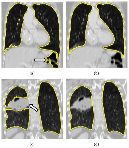
Quantitative analysis of medical images is essential for efficient utilization of medical image data in medicine. Medical image segmentation is often the first step of the quantitative analysis. Manual segmentation of organs in medical images requires the user to delineate/draw object boundaries. This is a tedious and time-consuming process. For example, manual lung segmentation in high-resolution multi-detector computed tomography (MDCT) images can take more than six hours. In the past, methods for automated segmentation were developed, but such methods can fail to produce correct segmentations of normal and especially diseased organs like for example the lungs depicted in Figs. 1(a) and 1(c). An important observation in this context is that segmentation errors are frequently bound to local regions. Consequently, it is accepted (best) practice in research and clinical applications to manually inspect and edit automatically generated segmentations to correct (local) segmentation errors (Figs. 1(b) and 1(d)). Doing so is more efficient than reverting to a pure manual segmentation. However, manual editing can still be time-consuming and is a limiting factor for utilization of quantitative lung image analysis in clinical and research applications.

Figure 1.

Example of fully automated lung segmentation results and corresponding results after manual slice-by-slice editing. (a) Normal lung where the segmentation leaked into the gas-filled colon (arrow) and (b) manually corrected segmentation. (c) Diseased lung with automatically generated segmentation result. The segmentation does not include cancer tissue (arrow) that is part of the lung. (d) Result after manual correction of this error.

In this paper, we address the issue of efficient editing of segmentations, which were generated by an automated graph-based optimal surface finding (OSF) method [1, 2]. Specifically, we propose a solution for more time-efficient editing of lung segmentations. The OSF-based segmentation approach guarantees global optimality of the resulting 3-D, 4-D, or generally n-D result according to a given cost function. In the literature, a number of OSF-based segmentation applications can be found. For example, methods for airway wall segmentation [2], simultaneous segmentations of bladder and prostate in 3-D CT scans [3], liver segmentation in 3-D CT scans [4, 5], segmentation of lungs with large lung cancer masses in 3-D CT scans [6], cartilage segmentation of the knee joint in 3-D MRI scans [7], femoral head and acetabulum segmentation [8], segmentations of retinal layers in 3-D retinal Optical Coherence Tomography (OCT) scans [9, 10], and finding of abnormalities in volumetric optical coherence tomography (OCT) images [11, 12] were reported. However, it is a nontrivial problem to find a suitable cost function for a specific segmentation problem. A cost function may work for the majority of cases, but some anatomical and pathological variation might cause the automated OSF segmentation to fail in a local region (Fig. 2). To correct the local failure of the automated OSF-based segmentation, effective interactive refinement methods are required. Once the initially problematic segmentation is refined, it can be utilized for further processing or analysis.

Figure 2.

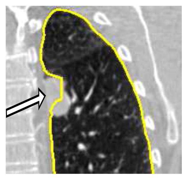
Example of a local OSF segmentation error (arrow) due to lung pathology (cancer). The employed OSF cost function is not well suited to successfully handle such pathology.

Interactive segmentation or segmentation refinement for 3-D medical data sets can be used when automated segmentation algorithms are not successful. A number of such techniques and tools were proposed in literature. For example, the 2-D live-wire segmentation method presented in [13] is a popular interactive segmentation approach, utilizing a conventional desktop (2-D) user interface. A 3-D extension of 2-D live-wire was presented in [14], but requires user interaction in many cross-sectional images. Slice-by-slice based interactive segmentation is tedious, time consuming and error prone, especially in the case of large image data sets. Schwarz et al. [15] proposed an interactive surface editing framework to refine the result of a 3-D Active Shape Model (ASM) segmentation utilizing a 2-D user interface.

In contrast to conventional user interfaces, a Virtual Reality (VR) based (3-D) user interface, which provides stereoscopic visualization and six degrees of freedom (6 DOF) input devices, allows true depth perception and natural interaction with objects or surfaces. A true 3-D interactive region growing approach presented in [16] is an early attempt to use a VR environment for segmentation. Harders et al. [17] performed tubular structure detection utilizing a desktop monitor based VR environment and tactile feedback. Deformable model based mesh surface editing tools with a hybrid VR/desktop user interface were introduced by Bornik et al. in [18]. As demonstrated in a recent study on liver segmentation [19], segmentation refinement performed with VR-based tools was found less time consuming compared to standard 2-D refinement. In [18] and [19], refinement is solely driven by the user without utilizing image segmentation algorithms during refinement. Thus, the user needs to manually “drive” the surface to match object boundaries visible in the image data.

In this work, we presented a novel interactive 3-D segmentation refinement method based on the OSF segmentation framework. The basic idea behind this method is that the user interacts directly with a segmentation algorithm to effectively correct potential errors in automatically generated OSF segmentation results. Our approach utilizes a hybrid desktop/VR user interface. The proposed method was validated in the context of lung segmentation in volumetric CT scans.

The paper is organized as follows. First, we briefly review the automated OSF segmentation framework. Second, we describe the utilized hybrid desktop/VR user interface used for refinement. Third, we present the interactive OSF-based refinement approach. Fourth, we evaluate our approach. Finally, we presented a discussion and conclusion.

2. Methods

2.1. OSF-based Segmentation

In the work presented in this paper, we assume that an initial segmentation was generated with an OSF segmentation approach that may yield local segmentation errors and thus may require refinement. The proposed refinement approach builds on the initially utilized OSF framework, but allows the user to locally guide the segmentation result.

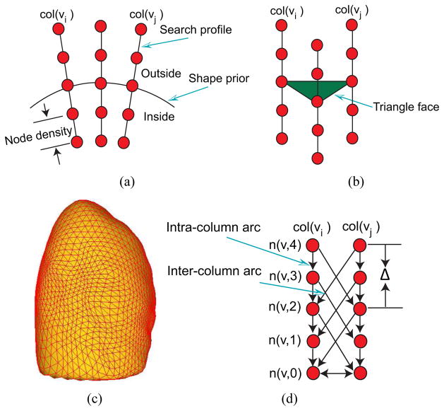
The main idea of the OSF-based segmentation algorithm is to transform the segmentation problem into a graph optimization problem. To utilize the OSF-based segmentation framework proposed by Li et al. [2], a weighted graph G(N, A) is built from an initial mesh surface M(V, F) (shape and topology prior) close to the target surface, where N represents a graph node set, A a graph arc set, V a triangle vertex set, and F a triangle face set, respectively. For each vertex v ∈ V, a graph column with l_p nodes is generated along the search profile. The direction of the search profile goes from inside to the outside of the segmented object. The node density on the profile is d_n and is adjusted to the given image resolution. Intra-column arcs are built to connect nodes n(v, k) to n(v, k − 1) on a column col(v) with infinity weights, where k is the column node index. Column col(v_i) and col(v_j) are adjacent columns, if vertices v_i and v_j are on the same triangle edge. For adjacent columns, inter-column arcs are built to connect the node n(v_i, k) to the node n(v_j, k − Δ) with infinity weights. Here Δ is the hard smoothness constraint, reflecting the largest allowed difference in nodes between two adjacent vertices. An example of such graph representation is shown in Fig. 3. The graph node weights C (cost function) are derived from volumetric image data to describe local image characteristics. The segmentation task is transformed to find a minimum-cost closed set by means of a maximum-flow algorithm [20]. To define a minimum-cost closed set problem, node costs are transformed into s-t arc capacities. A node weighted graph eventually becomes an arc weighted graph. The feasible surface is the envelope of the minimum-cost closed set.

Figure 3.

Graph construction of a single-surface segmentation problem in the OSF framework. (a) Search profiles are constructed starting from the shape prior. (b) Relation between search profiles and triangle face of the shape prior. (c) Example of the shape prior (pre-segmentation) used for OSF-based lung segmentation. (d) OSF graph structure with arcs enforcing the surface smoothness constraints.

2.2. User Interface

We utilize a combination of desktop (2-D) and VR (3-D) user interfaces similar to the work reported in [18]. Refinement can be accomplished by using a stereoscopic display with a tracked (6 DOF) input device or a standard 2-D interface (e.g., monitor and mouse) for more accurate control. The hybrid user interface reported in [18] utilized a distributed architecture with two computers. Thus, all operations, data, and visualizations needed to be synchronized over the network between 2-D and 3-D user interface computers. The drawback of such an approach is that large data sets might slow down communication and lead to low frame rates, besides potential network latency issues. Since a responsive system with high frame rates is essential for an interactive VR system, we have developed a hybrid user interface where 2-D and 3-D interfaces are implemented on the same machine.

2.2.1. Hardware Setup

The hardware setup consists of several components and includes an active stereo display, an optical tracking system, a Wacom interactive pen display (Wacom Co., Ltd., Japan), and a graphics workstation (Fig. 4). A Mitsubishi 3-D DLP HDTV with 73 inch diagonal, 1920 × 1080 pixels, and a refresh rate of 120 Hz was utilized as active stereo display. It was operated in the side by side stereo mode in combination with Nvidia 3-D Vision (Nvidia Corp., Santa Clara, CA) stereo shutter glasses (Fig. 4(a)). The stereo display and Wacom display are driven by a Linux workstation with four 6-core 2.93 GHz Xeon CPUs and a Nvidia Quadro Fx 5800 graphics card (Nvidia Corp., Santa Clara, CA). The 6 DOF input device (Fig. 4(a)) built for 3-D and 2-D user interaction consists of a Bluetooth mouse, a Wacom display stylus, and an optical tracking target. The optical tracking system (NaturalPoint Inc., Corallis, OR) includes a tracking server and five optical tracking cameras, which track the user’s head, the stereo display, and the input device (Fig. 4(a)). The tracking system software is running directly on the graphics workstation, and tracking data are transported from tracking server to our developed software via a loopback device.

Figure 4.

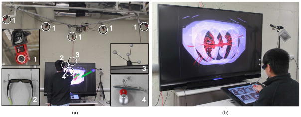
Hybrid user interface for interactive OSF segmentation refinement. (a) The user inspects the segmentation result by utilizing a 3-D user interface. Circled devices are shown in enlarged sub-figures: (1) tracking cameras, (2) shutter glasses with head tracking targets, (3) stereo display with tracking targets, and (4) tracked input device. (b) The user operates the 2-D user interface. (a) (b) (c)

2.2.2. Software Architecture

The developed system utilizes Studierstube [21] and OpenTracker [22] to implement the VR system. Studierstube is a C++ library developed for Augmented Reality (AR) and VR applications. OpenTracker software is utilized for handling tracking data. Specifically, we use the Virtual Reality Peripheral Network (VRPN) protocol to transmit the tracking data. Studierstube forwards tracking data from OpenTracker to our application. We extended the original Studierstube library to support side-by-side stereo rendering mode required by the 3-D DLP TV.

2.2.3. Visualization Algorithms

Visualization tools facilitate the inspection of segmentation results and interactive refinement of segmentations, if needed. The VR user interface utilizes a textured cutting plane, a form of a multi-planar reconstruction (MPR), for displaying volumetric context data. For this purpose, OpenGL 3-D texture is utilized. In our system, segmentations are represented by triangle meshes. In a refinement task, the operator uses the 6 DOF input device to place the MPR and inspect arbitrary 2-D views on the MPR in combination with the mesh surface. However, the rendering of surfaces and a MPR are inadequate to observe local details. Thus, a 2-D contour resulting from the intersection of the mesh surface with the MPR can be visualized, if needed. In this contour rendering mode, the MPR is used as a clipping plane.

The contour rendering is essential for verifying the segmentation result. However, the mesh surface can consist of many triangles, and MPR location/orientation and the surface are subject to frequent changes. Thus, a fast contour rendering method is required. For this problem, Bornik et al. [18] proposed a two-pass image based contour rendering algorithm. First, the algorithm renders the clipped surface in two-sided light mode to the OpenGL Frame Buffer Object (FBO) buffer, which is used to generate an image with a white cross section of the clipped surface on a black background. Second, edge detection is used to extract the boundary. This approach has some disadvantages. If there are holes in the surface (e.g., open surface) or the orientation of some polygons is flipped (e.g., due to mesh folding), artifacts in the form of false silhouettes can appear (Fig. 5(a)). Also, this algorithmis not able to highlight a portion of the contour with a different color, which is required by our refinement method.

Figure 5.

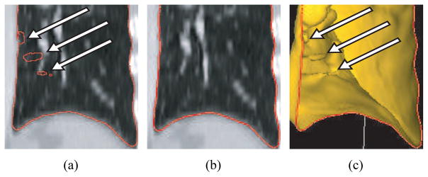
Comparison of the visualization approach presented in [18] (a) and our proposed method (b). (a) False contours are clearly visible on the cutting plane. (b) Our algorithm produces a correct contour. (c) The contour shown in (b) is combined with the clipped mesh. Arrows show locations of mesh folding.

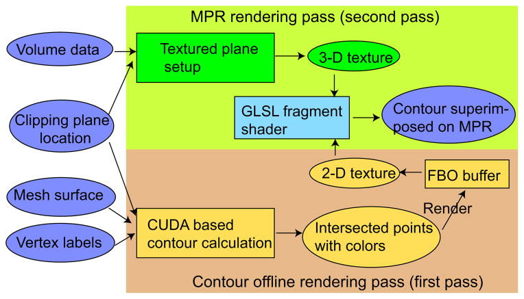
To address these problems, a CUDA¹ based contour visualization algorithm was developed. Fig. 6 provides an overview of the algorithm. In our approach, we assume that each mesh vertex has a label corresponding to a color. In the first pass (Fig. 6), the intersection points of the mesh surface and MPR (clipping plane) are calculated in parallel. In the CUDA implementation, a thread is generated for each triangle and delivers zero or two intersection points of the triangle with the clipping plane. Note that without loss of generality, the case with only one intersection point can be represented with two intersection points. Each intersection point is labeled according to the set label of the nearest triangle vertex. Thus, each intersection point is assigned a color according to its set label. Two intersection points are drawn as a line and finally rendered into the FBO buffer as 2-D texture. In the second pass (MPR rendering pass depicted in Fig. 6), the 2-D texture is superimposed onto the textured plane representing the image context utilizing an OpenGL Shading Language (GLSL) fragment shader program. Thus, the contour is always shown on the textured plane without any occlusion. Note that if the two intersection points were assigned different colors, the color of the line in between will be interpolated accordingly.

Figure 6.

Overview of the contour rendering algorithm.

Fig. 5 shows a comparison between our result and a result generated with Bornik’s algorithm [18]. Fig. 7(b) and Fig. 7(c) depict another example of the application of the contour rendering algorithm in the context of segmentation refinement.

Figure 7.

Visualization of generic interactive OSF-based segmentation refinement for a lung with a lung mass adjacent to the lung boundary. (a) The user inspects the lung segmentation and locates a segmentation error. (b) In a cross-section, the user selects a point on the correct boundary location with a virtual pen. Note that the incorrect portion of the contour is highlighted in light blue and was automatically generated based on the selected point. (c) and (d) Refinement result after calculating maximum-flow. (d) The corrected surface region is highlighted in green.

2.3. Generic OSF-based Segmentation Refinement

Our segmentation refinement method utilizes the same graph structure G(N, A) as described in Section 2.1. In this context, note that our method does not change the topology of the underlying graph structure. Basically, the task of segmentation refinement can be split into two sub-tasks:

1. identify (label) the local error on the surface and

2. change the cost of columns associated with errors such that the error is corrected or at least reduced when the new optimal surface is calculated for the updated graph.

In this context, it is desirable that user interaction is minimized for both sub-tasks.

The individual processing steps of the developed segmentation refinement algorithm are as follows.

1. The user inspects the segmentation result and detects an error on the surface by comparing CT data visualized on the cutting plane to the boundary of the segmentation result (Fig. 7(a)).

2. The incorrect part of the surface is labeled. For this purpose, the user identifies a point on the true surface location near the error region (Fig. 7(b)). During this process, the algorithm displays the estimated incorrect (labeled) portion of the surface interactively. This allows the user to pick a good location for the input point.

3. Costs in G(N, A) are locally updated for affected columns.

4. The maximum-flow is recalculated for the graph G(N, A). To speed up the computation, we avoid to recompute the maximum-flow from scratch and utilize the previously calculated residual graph instead, similar as described in [23].

5. The new solution (surface) is displayed (Fig. 7(c) and 7(d)).

The above described refinement method can be utilized iteratively, if needed. The refinement process is supported by the hybrid user interface and the visualization tools presented in Section 2.2. In the following, we describe step 2 and step 3 of our refinement algorithm in detail.

Error region labeling (step 2)

The user specifies a point on the true boundary in an erroneous segmentation region using the hybrid user interface (Fig. 7(b)). The algorithm searches for the nearest node on all graph columns based on the specified point. The nearest node n(v, k) is found. Corresponding column v is labeled as the center column, and the center column node n(v, i) on the previously calculated surface is found (Fig. 8). A breadth-first-search (BFS) algorithm [24] is applied to find similar neighboring columns. The neighborhood relation is defined based on mesh topology. The BFS starts from the center column v and examines neighboring columns by utilizing predefined similarity criteria, which are based on three components that are combined by means of a logical AND operation:

Figure 8.

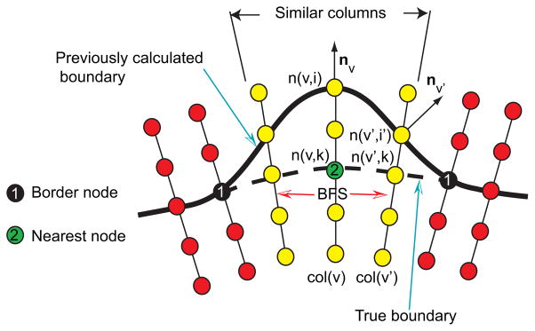
Search for similar neighboring columns in the OSF graph structure.

1. Surface normal vector direction — To limit the search to a local region with roughly similar surface orientation, we require that the angle between mesh surface normal vectors of the center column v and a neighboring column v′ must be less than 90°, and thus, fulfill n_v · n_v′ > 0, where n denotes the surface normal (Fig. 8).

2. Gray-value characteristics of the incorrect surface boundary — This criterion is based on the observation that the incorrect surface passing through the center and the neighboring columns should have similar local image characteristics. The gray-value profile around a node n(v, i) will be denoted as set P(v, i) = {g(n(v, i + j))| j ∈ {−7, −6, …, 7}}, where g(n) represents the gray-value of a node n. Let v′ represent a column in the proximity to the center column with node n(v′, i′) on the previously calculated surface (Fig. 8). Then D(P(v, i), P(v′, i′)) = max_{j∈{−7,−6,…,7}}{|g(n(v, i − l_r + j)) − g(n(v′, i′ + j))|} denotes a gray-value profile similarity function. Columns v and v′ are similar if the following criterion is fulfilled:

   $$\underset{m\in \{-5,-4,\dots ,5\}}{min}\{D(P(v,i),P(v^{\prime },i^{\prime }+m))\}<t_1,$$ (1)

   where t₁ is a threshold. In our lung CT segmentation task, we use t₁ = 180 HU (Hounsfield Units).

3. Gray-value characteristics of the true boundary location — The basic idea behind this criterion is that the correct surface point(s) on the center column and neighboring columns have similar gray-value appearance. The correct surface point n(v, k) on the center column was selected by the user (Fig. 8). However, we need to search for the correct surface points on neighboring columns. For the neighboring column v′, we start the search from n(v′, k) (Fig. 8) with a variable search length

   $$l_t=\mathit{round}(5+7(1.0-e^{\frac{-d_{v,v^{\prime }}^2}{2{\sigma }^2}}))$$ (2)
   to express increasing uncertainty regarding location of true boundary points with increasing distance from column v. Here, d_v,v′ denotes the Euclidean distance between previously calculated surface nodes on column v and v′; σ was set to 5 mm. Columns v and v′ are similar if

   $$\underset{m\in \{-l_t,-l_t+1,\dots ,l_t\}}{min}\{D(P(v,k),P(v^{\prime },k+m))\}<t_2,$$ (3)

   Threshold t₂ was set to 90 HU. The node with the most similar gray-value profile on column v′ is stored in a set V_sim.

After the BFS algorithm stops, holes are filled in the labeled surface. Nodes corresponding to the surface patch are stored in the set V_err. Fig. 7(b) shows an example of a labeled erroneous surface patch visualized on the cutting plane. Parameters for the similarity criteria were selected conservatively to avoid leakage. Thus, the BFS step might in some cases not completely label the incorrect surface patch. To address this issue, the patch can be dilated by the user.

Updating OSF costs (step 3)

The cost function of the center column is updated by

$$c(v,i)=\{\begin{array}{cc}10\hfill & ifi\ne k\\ 0\hfill & i=k\end{array}.$$ (4)

Because all costs are initially normalized between 0 and 1, the final segmentation is very likely to pass through the user determined location k on column v. All remaining columns related to the set V_err are updated with

$$c(v^{\prime },i)=\{\begin{array}{cc}{c}_t(v^{\prime },i)\hfill & if{v}^{\prime }\notin \mathrm{\Omega }\\ c(v^{\prime },i)\hfill & \mathit{otherwise}\end{array},$$ (5)

where Ω is a set containing all center columns selected by the user during the refinement process. Thus, the refinement never changes the cost function of columns already updated using Eq. 4 in the previous refinement steps. The term

$$c_t(v^{\prime },i)=\left(1.0-0.5e^{\frac{-{(\mid i-k^{\prime }\mid )}^2}{2\sigma {(v,v^{\prime })}^2}}\right)c(v^{\prime },i)$$ (6)

is used to locally adapt the previously utilized costs, where node k′ represents an estimate for the true boundary location on column v′. The estimation of k′ will be described in the next paragraph. σ(v, v′) is calculated with $\sigma (v,v^{\prime })=5+e^{\frac{d_{{vv}^{\prime }}}{10}}$. The idea behind Eq. 6 is that the costs on column v′ near to the node n(v′, k′) have to be low while the impact of the weighting function becomes weaker for nodes on columns that are further away from n(v′, k′).

The estimate for the true boundary node n(v′, k′) is calculated as follows. Let V_border denote a set of outer border nodes of V_err (Fig. 8). A Thin Plate Spline (TPS) surface [25] is fit through user selected node n(v, k), nodes in V_border, and nodes in Ω_sim. To speed-up computation, ω_sim is a randomly selected subset of V_sim with 20 % of the size of V_sim. We utilize a TPS interpolation because we assume that the corrected surface has low shape complexity. For TPS interpolation, the kernel function U(r) = r² log r is utilized. The interpolation works in 2.5D while the surface patch consists of 3-D points. Thus, an appropriate 2-D plane has to be found to apply TPS interpolation. By means of singular value decomposition, a plane is fitted in a least square fashion to nodes in V_border. The intersection of the interpolated surface and columns related to set V_err\{n(v, i)} form estimates for the true boundary.

Note that n(v, k) and nodes in V_border are believed to be on the true surface, but nodes corresponding to Ω_sim were estimated. Therefore, we enforce the fitted surface to pass through nodes n(v, k) and V_border with a regularization parameter value of 0, but do not enforce it through nodes related to Ω_sim with a regularization parameter value of 1.0 [26].

Note that parameters used in the described method were determined experimentally on five cases, which were not included in test data sets. An example of generic OSF-based interactive segmentation refinement is given in Fig. 7.

2.4. Specific OSF-based Refinement Method for Leakage to Trachea and Main Bronchus

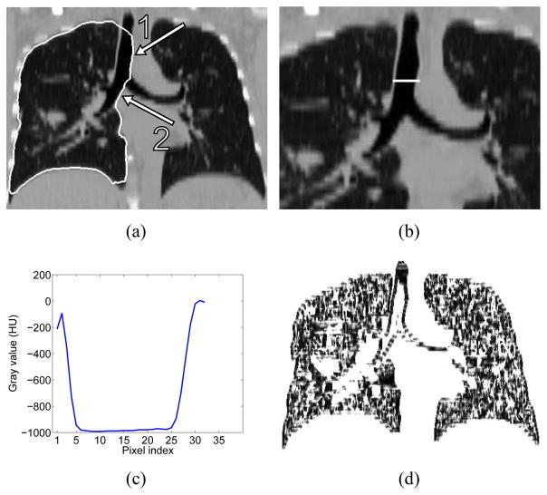
The tool described in Section 2.3 is well suitable to correct lung segmentation errors. However, we observed that when the OSF based lung segmentation leaks to the trachea and main bronchus (Fig. 9(a)), the method is not efficient, requiring the user to specify too many refinement points. To address this issue, we designed a specific tool for this segmentation problem. This specific method also consists of 5 steps as described in Section 2.3, but step 2 (error region labeling) and step 3 (updating OSF costs) are different from the generic approach. In the next sections, these steps are explained in detail.

Figure 9.

Example of incorrect lung segmentation (leakage to trachea and main bronchus) and corresponding image features utilized for error identification. (a) Lung segmentation leaking to trachea (arrow 1) and main bronchus (arrow 2). (b) Profile location and (c) corresponding gray-value profile passing through airway lumen and surrounding tissues. (d) Corresponding z · g_dir volume.

Error region labeling (step 2)

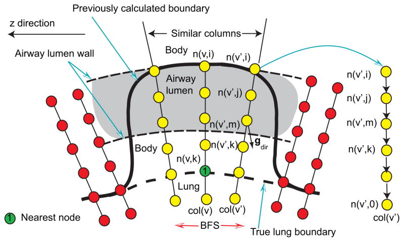
The basic idea is to utilize the gray-value and gradient characteristics of CT image data to identify/label surface points corresponding to the leak to trachea and the main bronchus. The center column node n(v, k) (nearest node in Fig. 10) is found based on the manually selected point on the true lung boundary in the area of the leak. The BFS algorithm is utilized to identify the incorrect nodes and is based on two properties:

Figure 10.

Labeling surface points corresponding to the leakage to trachea and main bronchus based on BFS.

1. Gray-value properties — A large density difference between air-filled airway lumen and surrounding tissue can be observed. Fig. 9(c) shows a typical gray-value profile passing through the airway lumen and surrounding tissue corresponding to the profile shown in Fig. 9(b). Columns involved in the leakage to trachea and main bronchus pass through the airway lumen as illustrated in Fig. 10. Thus, for the neighboring column v′, nodes starting from n(v′, i) to n(v′, 0) are searched (Fig. 10) and their average gray-values $g_a(v,i)=1/7{\sum }_{j=-3}^{3}g(n(v,(i+j))$ are examined. The averaging is used to reduce the influence of noise. At first, the search looks for a node n(v′, j) with g_a(v′, j) < −900 HU (air). Once such a node is found, the search continues on the column until the first node n(v′, k) with g_a(v′, k) > −600 HU is found. The node n(v′, k) will be close to the inner airway boundary (Fig. 10). The search is refined by identifying the maximal gradient magnitude location about node n(v′, k) in a search range of ±3 nodes, resulting in node n(v′,m). Gradient magnitude g_mag and direction g_dir are pre-calculated for each voxel in the volume. Prior to gradient calculation, the gray-value range is truncated to −1000 and −700 HU, to reduce the effect of unrelated structures on the gradient. The gradient is calculated by utilizing Gaussian derivatives with a standard deviation σ_g = 0.5 mm. In addition, to reduce the influence of noise, gradient magnitudes less than 10 are ignored. The same search is performed for the center column, but it takes place between nodes n(v, i) and n(v, k).

2. Gradient properties — Trachea and main bronchus are elongated tubular structures along the z-axis of the volume. Thus, the z-axis is approximately perpendicular to the (normalized) gradient direction of each voxel on the airway boundary. This constellation can be described by the dot product z · g_dir, where z = (0, 0, 1)^T represents the z-axis direction and g_dir = (g_x, g_y, g_z)^T is the normalized gradient direction of each voxel. Fig. 9(d) shows a typical example of a z · g_dir volume.

The criterion is fulfilled if a node n(v′,m) can be found for a neighboring column with z · g_dir(n(v′,m)) < t₃ with the angle threshold t₃ = 0.4. After the BFS algorithm stops, nodes corresponding to the surface patch are stored in the set V_err, and holes in the patch are closed. In addition, nodes on the airway wall (n(v′,m)) are stored in the set V_sim. For columns related to holes in the surface patch, the location of the node n(v′,m) is estimated by interpolation, and the result is added to V_sim.

Updating OSF costs (step 3)

The cost function of the center column is updated according to Eq. 4. All other columns corresponding to nodes in V_err are updated by Eq. (5) as

$$c_t(v^{\prime },i)=\{\begin{array}{cc}1\hfill & ifi>m\\ c_0(v^{\prime },i)\hfill & \mathit{otherwise}\end{array},$$ (7)

with n(v′,m) ∈ V_sim. c₀(v′, i) is the initial cost function utilized before refinement. Thus, nodes inside the airway lumen receive a cost of one.

3. Evaluation Methodology

3.1. Image Data

For our study, 18 multidetector computed tomography (MDCT) thorax scans of patients with lung tumors were selected from a larger pool of data sets such that at least the left or right lung required segmentation refinement after automated segmentation (Section 3.3). In the 18 MDCT scans, 21 left/right lungs were found to require segmentation refinement. MDCT images where acquired with different scanners and imaging protocols. The image sizes varied from 512 × 512 × 415 to 512 × 512 × 642 voxels. The slice thickness of images ranged from 0.6 to 0.7 mm and the in-plane resolution from 0.60 × 0.60 to 0.79 × 0.79 mm. None of the test data sets has been used for the development of algorithms.

3.2. Independent Reference Standard

For all tested data sets, an independent reference standard was generated by following the current standard procedure utilized in numerous large multi-center research projects as well as clinical applications. First, an automated lung segmentation was performed by utilizing a commercial FDA 510K approved lung image analysis software package PW2 (VIDA Diagnostics Inc., Coralville, IA). Second, since the software was not designed to deal with lungs containing large lung cancer regions, an expert inspected all the segmentations slice-by-slice and manually corrected all segmentation errors. In the case of diseased lungs, this process took several hours per lung.

3.3. Initial Automated Lung Segmentation

For automated segmentation, we adapted the approach proposed by Sun et al. [6]. The lung segmentation uses a robust ASM based segmentation followed by an OSF-based segmentation approach. In [6], Sun et al. utilized a multi-scale OSF approach with a hard smoothness constraint [2] and straight line search profiles normal to the mesh surface. For the experiment reported in this paper, we utilized an improved version of this algorithm that included a linear soft smoothness constraint (a constant weight α was used to penalize the shift on two adjacent vertices on the final feasible surface) proposed in [3] and a gradient vector flow based approach to build column profiles [27]. Also, in contrast to [6], we used a single-scale approach. The number of mesh vertices used for the OSF-based segmentation was 10, 242. For the soft and hard smoothness constraints, α = 0.001 and Δ = 12 were used, respectively. The search profile length was l_p = 117 nodes. Points on the search profile were obtained at discrete sampling positions with a distance of 0.35 mm between them. A Gaussian gradient filter kernel with variance σ = 2.0 mm was utilized to calculate the cost function as outlined in [6].

3.4. Identification of ROIs for Performance Analysis

To assess segmentation refinement performance, 30 volumetric region of interests (ROI) were identified in the images that contained major local segmentation errors. The approach for generating ROIs was as follows. First, an exclusive OR operation was applied to the volumetric lung masks of the independent reference standard (Section 3.2) and initial automated segmentation (Section 3.3) to generate a volume that depicts the differences between both segmentations. A morphological erosion operation was applied to remove smaller regions. The remaining large regions were morphologically dilated to form ROIs that include major segmentation errors (Fig. 11). These ROIs were also utilized to indicate, which region should be refined by the user. Table 1 summarizes segmentation error types included in the defined ROIs. Note that there can be one or more types of segmentation errors in a single ROI. An expert was asked to refine the segmentation errors inside the ROIs.

Figure 11.

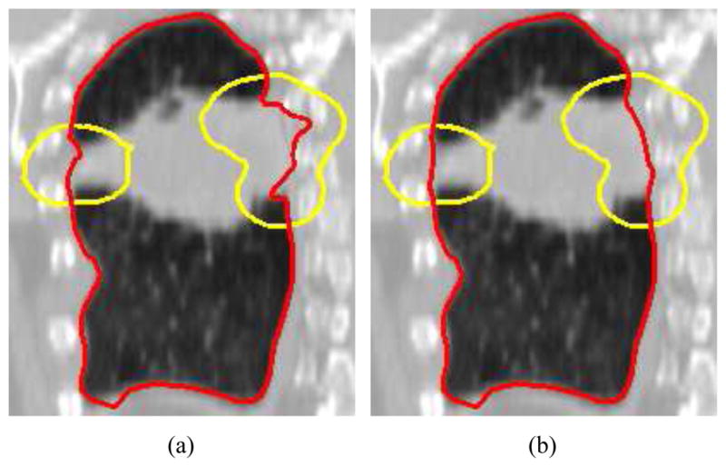
A comparison of segmentation before (a) and after (b) refinement. The segmentation is highlighted in red and the ROI region is shown in yellow. (a) Initial automated OSF segmentation. (b) Corresponding 3-D segmentation refinement result.

Table 1.

Summary of segmentation error types included in the predefined ROIs. Note that only major segmentation problems in ROIs were taken into account.

Error location	Frequency
cancer region	12
leak to high contrast region (e.g., contrast agent)	12
leak to airway branch & hilar region	5
leak to trachea and main bronchi	2

3.5. Quantitative Indices

The utilized ROIs were defined such that the segmentation errors can be corrected by manipulating the surface portion inside the ROIs. However, the user might unintentionally affect a portion of the surface in close proximity to the ROI boundary or the global optimal OSF calculation might cause changes outside of the ROI. Therefore, we evaluate refinement performance inside and outside the ROIs.

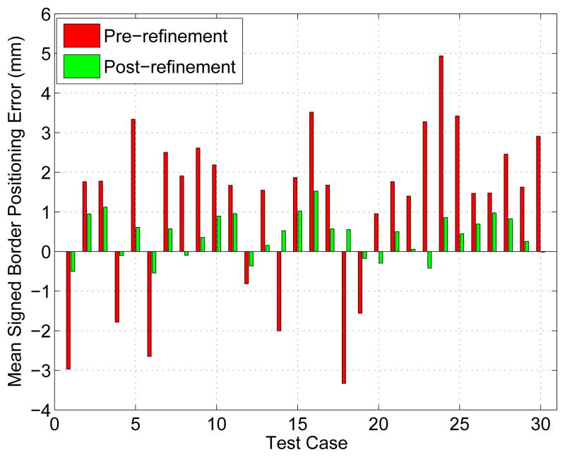
1. Validation inside ROIs — The following quantitative error indices were utilized: mean absolute surface distance (d_a) [28] and mean signed border positioning errors (d_s) [29]. A negative value for d_s indicates that the segmentation boundary is inside the reference object and a positive value indicates that the boundary is outside the reference object.

2. Validation outside ROIs— The Euclidean distance (d_e) of two corresponding surface vertices before and after refinement are utilized to measure vertex displacement. In addition, for each refinement-modified vertex outside the ROI, a shortest geodesic distance (d_g) to the ROI boundary is utilized to measure proximity to the ROI. To calculate d_g, a weighted undirected graph G_dg is constructed from the triangle mesh. The arc weight is based on the Euclidean distance between two triangle vertices. d_g is calculated based on Dijkstra shortest path algorithm [24].

In addition to the above outlined indices, the user interaction and algorithm computing time required for refinement per ROI was recorded.

4. Results

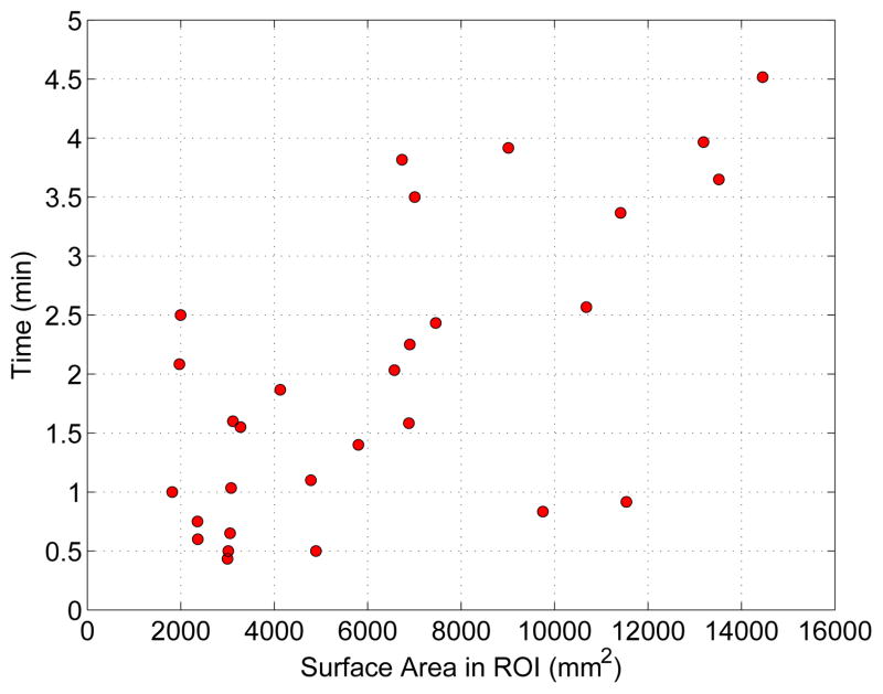
The mean and standard deviation of user interaction times needed for segmentation refinement per ROI was 1.9 ± 1.2 min with a median of 1.6 min. User interaction times ranged between 0.4 and 4.5 min. On average 5 ± 3.4 (median: 4) manually defined surface-correcting points were required, and the minimum and maximum were 1 and 13 points, respectively.

A plot of required interaction in dependence of surface area inside the ROI is depicted in Fig. 12. The actual computing time required by the algorithm was 150 ± 152 ms (median: 101 ms) with minimum and maximum computing time of 73 and 1220 ms, respectively.

Figure 12.

User interaction times required for each refinement task in dependence of surface size inside the ROI. Note that conventional approach to correcting severe segmentation failures using slice-by-slice contour editing tools typically require tens of minutes and up to several hours per image dataset.

4.1. Results inside ROIs

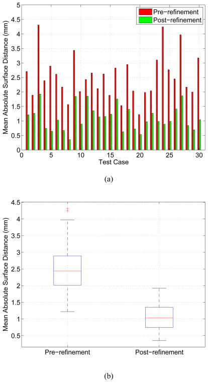
The mean absolute surface distance and mean signed border positioning errors before and after refinement measured inside ROIs for all thirty test cases are shown in Figs. 13 and 14, respectively. A Student’s t-test at a significance level of 0.05 was performed to determine whether the average error indices after refinement were significantly different than prior to the refinement. Both indices, the mean absolute surface distance (p ≪ 0.001) and mean signed border positioning error (p = 0.02), were significantly improved. The mean absolute surface distance errors prior to the refinement were 2.54 ± 0.75 mm (median: 2.44 mm) and the same errors decreased to 1.11 ± 0.43 mm (median: 1.04 mm) after the refinement. Fig. 13b shows boxplots graphically demonstrating improvements in the surface distance errors after refinement.

Figure 13.

Mean absolute surface distance error before and after segmentation refinement measured inside the ROIs. (a) A case by case comparison. (b) A boxplot comparison summarizing performance in all tested cases. The boxplot is a graphical display of a five number summary (from bottom to top vertical line): the so-called smallest observation (Q₁ − 1.5(Q₃ − Q₁)), first quartile (Q₁), median (Q₂), third quartile (Q₃), and the so-called largest observation (Q₃ + 1.5(Q₃ − Q₁)); + marks indicate outliers.

Figure 14.

Mean signed border positioning errors before and after segmentation refinement measured inside the ROIs.

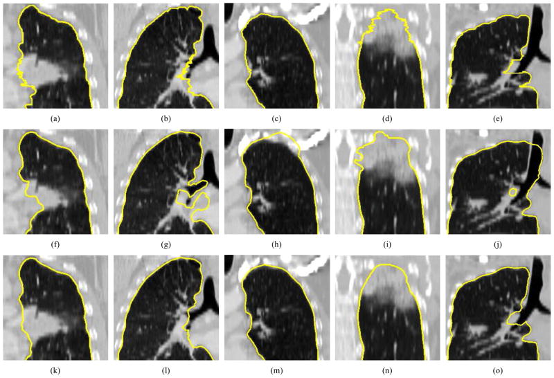
Examples of segmentations before and after refinement are depicted in Figs. 11, 15, and 16. In the case of Fig. 16, the independent reference standard is also shown for comparison.

Figure 15.

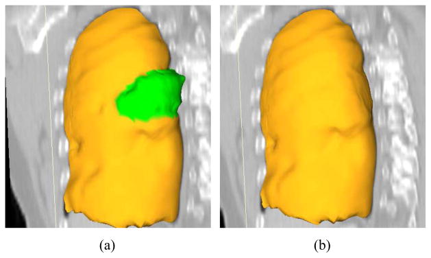
A comparison of automated segmentation and segmentation refinement in mesh representation for the case shown in Fig. 11. (a) Initial automated OSF segmentation. The region marked green indicates segmentation error due to a large lung cancer region. (b) Corresponding 3-D segmentation refinement result.

Figure 16.

Examples of segmentation results on five different data sets (columns). (a)–(e) Independent reference standard. Note that a zigzag pattern of the reference boundary can be observed on both the sagittal or coronal views, because the manual expert segmentation was performed in a slice-by-slice fashion and typically leads to slice-by-slice inconsistencies. (f)–(j) Initial automated OSF segmentation results. (k)–(o) Segmentation after 3-D refinement.

4.2. Results outside ROIs

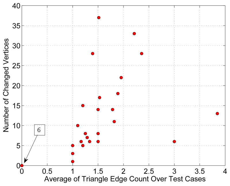
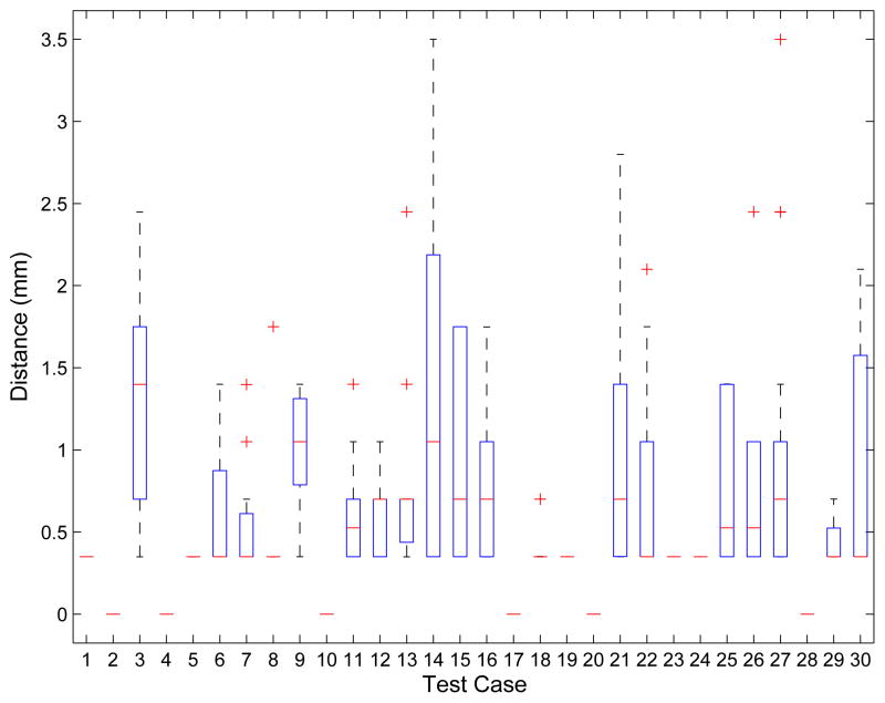
The impact of segmentation refinement on the segmentation outside the ROIs is summarized in Fig. 17, which shows a plot of the number of altered vertices as a function of the mean number of triangle edges on the ROI boundary. For each test case, boxplots for the displacement of nodes outside the ROIs after refinement are shown in Fig. 18. Combined over all 30 cases, the average node displacement was 0.56 ± 0.38 mm (median: 0.57 mm) with a range of 0 to 1.34 mm.

Figure 17.

Dependence between number of after refinement altered vertices outside the ROI and average triangle edge count on the geodesic shortest path from altered vertices to the ROI boundary. Note that six test cases are located at the origin of the coordinate system, as indicated by the arrow.

Figure 18.

Boxplot of the displacement distance of vertices outside the ROI that were altered during refinement. Note that for the six cases without displacement a red line at zero is shown.

5. Discussion

The optimal surface finding framework is a powerful approach and has demonstrated utility in a number of medical image segmentation problems, as outlined in Section 1. However, when dealing with segmentation of structures/organs that are abnormal due to disease or other causes, designing a suitable cost function that would work correctly for all possible situations is challenging and may be impossible since pathology augments image characteristics. As a consequence, segmentations can exhibit local errors. Such local inaccuracies or errors must be corrected prior to the subsequent quantitative analysis. For achieving full yield of medical imaging under all disease conditions, an efficient and inherently three-dimensional approach must be available in the workflow to facilitate efficient modification or refinement of the resulting segmentations. Clearly, the current state-of-the-art approach of slice-by-slice editing offers neither efficiency nor 3-D performance.

In this paper we have addressed this problem in the context of lung segmentation of volumetric CT scans. We have developed an OSF-based segmentation refinement system, which utilizes a virtual reality user interface to facilitate an efficient interaction with automatically-determined object/organ surfaces. We have demonstrated the feasibility and potential of such an approach.

The validation showed that the developed method allowed the user to successfully reduce/correct segmentation inaccuracies in all 18 test data set with 30 ROIs where the automated segmentation approach locally failed and interactive surface refinement was necessary (Fig. 13 and 14). Quantitative assessment of the achieved segmentation improvements demonstrated that the improvements are statistically significant.

Our 3-D refinement results show that the refined surfaces exhibit smooth boundaries (Fig. 16(k–o)), an additional benefit of our approach compared to slice-by-slice manual editing of 2-D contours, which shows surface inconsistencies (zig-zag lines) across slices (Fig. 16(a–e)). In addition, it is difficult to consistently define the lung boundary in the area near the hilum where vessels and airways enter/leave the lungs and no generally accepted standard for segmentation exist. In this context, it is interesting to note that in four out of the five test cases, for which the mean absolute surface distance after refinement exceeded 1.5 mm, required refinement in the hilum region, further stressing the difficulty of expert-determination of proper surfaces in this location of pulmonary anatomy.

Because the OSF approach delivers a globally optimal solution, a local manipulation of a cost function could potentially lead to an alteration of the solution (surface) outside of the local area where the cost function was purposely modified (i.e., surface changes may theoretically appear outside of the refinement ROI). The performed assessment of such change outside the predefined ROIs indicated that in our 18 datasets, only minor changes occurred in close proximity to the ROI region and no changes were detected in the remaining parts of the lung surface. This result suggests that the influence of the modifications remains local in practice and the global modifications possibility does not form a problem in the image segmentation refinement application.

The required user interaction time was in the low single-minute range. The plot shown in Fig. 12 suggests that the refinement times of more than 2.5 min were only required for inaccuracies affecting large portions of the lung surface. Manual editing of the segmentation error in a slice-by-slice fashion would take much longer, because manipulating a surface is more efficient than editing 2-D contours in a cross-sectional images.

The average computing time of 150 ms per refinement iteration demonstrates that our algorithm is well suited for real-time interactive use. The maximum computing time of 1, 220 ms or just little over one second was recorded for a case involving a large surface region and was mainly required for surface interpolation. To further increase the responsiveness of the interactive refinement environment, we plan to develop a parallel implementation of the interpolation steps using CUDA. Once in place, we expect interaction response times not exceeding 100 ms per interaction. This will provide the user with a truly real-time interactive feeling when using the surface refinement environment.

In our CT lung surface segmentation refinement application, the two refinement tools—one generic and one specifically designed for leaks to trachea/main bronchus—were sufficient to handle the full range of frequently occurring lung segmentation inaccuracies. In both cases, a single user selected point was utilized per refinement iteration. With this information, the cost function of a local region was automatically modified by weighting costs, and subsequently, the (automated) OSF segmentation algorithm was applied to refine/manipulate the initial segmentation result. This approach has three major benefits. First, the refinement is performed within the initial segmentation framework. Thus, the same constraints (surface smoothness) apply, and surface discontinuity is avoided. Second, user input as well as local image features are utilized at the same time during the refinement process. Third, with just a single point, a larger local surface region can be refined. However, depending on the application (e.g., type of the lung disease, the utilized imaging protocol, etc.), adaptation of the existing tools and/or development of new tools may provide further benefits.

A potential limitation of our OSF-based segmentation refinement approach is that the correct solution must be representable by the utilized graph structure, because only weights (costs) of the graph are modified during refinement. Consequently, no topology modification is possible. This issue can be addressed in two ways. One would yield segmentation refinement methods that also allow the user to locally modify the graph structure. This approach is demanding in terms of the required computational effort and may not be achievable in real-time. Another approach is to revert to refinement tools based on interactively user-modified deformable contour described in [18, 19]. While such an approach would offer a larger degree of flexibility, it would likely require more user interaction steps and thus increase the overall refinement times.

In this paper, we focused on a refinement approach for single surface OSF segmentation. However, similar methods can be developed for dual-surface or 4-D (single surface plus time) OSF segmentation. An adaptation to other graph-based segmentation approaches might not be straight forward, or such methods might have refinement/interaction solutions like for example graph cuts [23].

The utilized hybrid user interface allows the user to either utilize a standard desktop environment (mouse and monitor), a 3-D VR environment (6 DOF tracked input device and stereoscopic display), or a combination of both. During the reported experiments, we observed that the user utilized the VR environment most of the time. One reason for this might be that it is quite intuitive to select a cross-sectional plane (multiplanar reconstruction) such that it shows large portions of the incorrect contour. On the other hand, refinement is highly computer-aided and the user only needs to specify one or more points on the correct object contour to manipulate the surface. We found that the point placement is not critical for good results, as long as the user-specified points are located on the correct boundary. Thus it seems to be very likely that the same performance can be achieved even if only the desktop user interface is utilized. Training of users might also play a role in the context of setup preference. To answer questions regarding the optimal user interface for specific refinement tasks, detailed studies of human computer interface aspects need to be performed. The presented hybrid desktop/VR user interface positions us well to investigate these aspects in the future. Also, we expect that the complexity of refinement tasks and associated tools will increase over time. This will lead to a clear distinction between pros and cons of user interface options. Another aspect in this context is that virtual reality hardware as currently utilized in experiments is not widely available in clinical practice. However, resulting from the advances driven by computer gaming and home entertainment, the accessibility of the VR environment components is rapidly increasing with a rapid decrease in the associated cost. Therefore, we expect that such VR equipment will become commonplace in health care and will be utilized for a range of medical applications.

6. Conclusion

We have presented a new OSF-based interactive segmentation approach utilizing virtual reality technology. This approach was investigated in the context of lung segmentation in volumetric CT scans. For efficient interaction, a hybrid desktop/VR user interface was developed utilizing state-of-the-art stereoscopic visualization technology and advanced interaction techniques in the context of medical image segmentation. The effectiveness of our approach was demonstrated on 18 lung scans containing 30 predefined ROIs, which consisted of segmentation errors frequently appearing in automated OSF-based lung segmentation results. Experimental results showed lower segmentation error indices compared to the errors of the automatically generated segmentations. An average user interaction time of about 2 min per ROI was achieved with a low number of user interaction “clicks”. Our work demonstrates the achievable benefits resulting from graph-based segmentation refinement.

The presented principle is equally applicable to other segmentation problems and across imaging modalities. However, the individual refinement tools may require some adaptation to be optimal for an specific application. All in all, the reported approach may be useful for all cases, for which automated segmentation approaches fail in some – perhaps difficult or pathologic – cases. The reported 3-D interactive refinement approach is being extended to 4-D to contribute to simultaneous context-aware segmentation of two lung volumes associated with breathing, the TLC (total lung capacity) and FRC (functional residual capacity) lung scans. In addition, applicability of interactive OSF-based refinement for segmenting multiple surfaces simultaneously (e.g., inner and outer surfaces of intravascular ultrasound images) will be investigated in our future work.

References

- 1.Wu X, Chen DZ. Optimal net surface problems with applications. Proc. of the 29th International Colloquium on Automata, Languages and Programming (ICALP); LNCS; 2002. pp. 1029–1042. [Google Scholar]
- 2.Li K, Wu X, Chen D, Sonka M. Optimal surface segmentation in volumetric images - a graph-theoretic approach. IEEE Transactions on Pattern Analysis and Machine Intelligence. 2006;28(1):119–134. doi: 10.1109/TPAMI.2006.19. [DOI] [PMC free article] [PubMed] [Google Scholar]
- 3.Song Q, Wu X, Liu Y, Smith M, Bautti J, Sonka M. Optimal graph search segmentation using arc-weighted graph for simultaneous surface detection of bladder and prostate. Proc. of Medical Image Computing and Computer Assisted Intervention (MICCAI); LNCS; 2009. pp. 827–835. [DOI] [PubMed] [Google Scholar]
- 4.Heimann T, Mnzing S, Meinzer H-P, Wolf I. A shape-guided deformable model with evolutionary algorithm initialization for 3d soft tissue segmentation. In: Karssemeijer N, Lelieveldt B, editors. Information Processing in Medical Imaging, Vol. 4584 of Lecture Notes in Computer Science. Springer; Berlin/Heidelberg: 2007. pp. 1–12. [DOI] [PubMed] [Google Scholar]
- 5.Zhang X, Tian J, Deng K, Wu Y, Li X. Automatic liver segmentation using a statistical shape model with optimal surface detection. IEEE Transactions on Biomedical Engineering. 2010;57(10):2622–2626. doi: 10.1109/TBME.2010.2056369. [DOI] [PubMed] [Google Scholar]
- 6.Sun S, Bauer C, Beichel R. Automated 3D segmentation of lungs with lung cancer in CT data using a novel robust active shape model approach. IEEE Transactions on Medical Imaging. 2012;31(2):449–460. doi: 10.1109/TMI.2011.2171357. [DOI] [PMC free article] [PubMed] [Google Scholar]
- 7.Yin Y, Zhang X, Williams R, Wu X, Anderson DD, Sonka M. LOGISMOS-layered optimal graph image segmentation of multiple objects and surfaces: Cartilage segmentation in the knee joint. IEEE Transactions on Medical Imaging. 2010;29(12):2023–2037. doi: 10.1109/TMI.2010.2058861. [DOI] [PMC free article] [PubMed] [Google Scholar]
- 8.Kainmueller D, ans HL, Zachow S, Heller M, Hege H. Multi-object segmentation with coupled deformable models. Medical Image Understanding and Analysis. 2008:3438. [Google Scholar]
- 9.Àbramoff MD, Garvin MK, Sonka M. Retinal imaging and image analysis. IEEE Reviews in Biomedical Engineering. 2010;3:169–208. doi: 10.1109/RBME.2010.2084567. [DOI] [PMC free article] [PubMed] [Google Scholar]
- 10.Quellec G, Lee K, Dolejsi M, Garvin MK, Àbramoff MD, Sonka M. Three-dimensional analysis of retinal layer texture: Identification of fluid-filled regions in SD-OCT of the macula. IEEE Transactions on Medical Imaging. 2010;29(6):1321–1330. doi: 10.1109/TMI.2010.2047023. [DOI] [PMC free article] [PubMed] [Google Scholar]
- 11.Dufour P, Abdillahi H, Ceklic L, Wolf-Schnurrbusch U, Kowal J. Pathology hinting as the combination of automatic segmentation with a statistical shape model. In: Ayache N, Delingette H, Golland P, Mori K, editors. Medical Image Computing and Computer-Assisted Intervention MICCAI 2012, Vol. 7512 of Lecture Notes in Computer Science. Springer; Berlin/Heidelberg: 2012. pp. 599–606. [DOI] [PubMed] [Google Scholar]
- 12.Chen X, Niemeijer M, Zhang L, Lee K, Àbramoff MD, Sonka M. 3D segmentation of fluid-associated abnormalities in retinal OCT: Probability constrained graph-searchgraph-cut. IEEE Transactions on Medical Imaging. 2012 Mar; doi: 10.1109/TMI.2012.2191302. [Epub ahead of print] [DOI] [PMC free article] [PubMed] [Google Scholar]
- 13.Barret WA, Mortensen EN. Interactive live-wire boundary extraction. Medical Image Analysis. 1997;1(4):331–341. doi: 10.1016/s1361-8415(97)85005-0. [DOI] [PubMed] [Google Scholar]
- 14.Schenk A, Prause G, Peitgen H-O. Efficient semiautomatic segmentation of 3D objects in medical images. Proc. of MICCAI; 2000; 2000. pp. 186–195. [Google Scholar]
- 15.Schwarz T, Heimann T, Tetzlaff R, Rau AM, Wolf I, Meinzer H. Interactive surface correction for 3D shape-based segmentation. Proc. of SPIE Medical Imaging 2008: Image Processing; 2008. 69143O–69143O–8. [Google Scholar]
- 16.Senger S. Visualizing and segmenting large volumetric data sets. IEEE Computer Graphics and Applications. 1999:32–37. [Google Scholar]
- 17.Harders M, Wildermuth S, Szekély G. New paradigms for interactive 3D volume segmentation. Visualization and Computer Animation. 2002;13(5):85–95. [Google Scholar]
- 18.Bornik A, Beichel R, Schmalstieg D. Interactive editing of segmented volumetric datasets in a hybrid 2D/3D virtual environment. Proc. of the ACM symposium on Virtual reality software and technology; ACM; 2006. pp. 197–206. [Google Scholar]
- 19.Beichel R, Bornik A, Bauer C, Sorantin E. Liver segmentation in contrast enhanced CT data using graph cuts and interactive 3D segmentation refinement methods. Medical Physics. 2012;39(3):1361–1373. doi: 10.1118/1.3682171. [DOI] [PMC free article] [PubMed] [Google Scholar]
- 20.Boykov Y, Kolmogorov V. An experimental comparison of min-cut/max-flow algorithms for energy minimization in vision. IEEE Transactions on Pattern Analysis and Machine Intelligence. 2004;26(9):1124–1137. doi: 10.1109/TPAMI.2004.60. [DOI] [PubMed] [Google Scholar]
- 21.Schmalstieg D, Fuhrmann A, Hesina G, Szalavári Z, Encarnaçäo LM, Gervautz M, Purgathofer W. The Studierstube augmented reality project. Presence: Teleoperators and Virtual Environments. 2002;11(1):33–54. [Google Scholar]
- 22.Reitmayr G, Schmalstieg D. An open software architecture for virtual reality interaction. Proc. of the ACM symposium on Virtual reality software and technology; ACM; 2001. pp. 47–54. [Google Scholar]
- 23.Boykov Y, Jolly M-P. Interactive graph cuts for optimal boundary & region segmentation of objects in N-D images. Proc. of International Conference on Computer Vision; IEEE; 2001. pp. 105–112. [Google Scholar]
- 24.Cormen TH, Leiserson CE, Rivest RL, Stein C. Introduction to algorithms. MIT Press; 2009. [Google Scholar]
- 25.Bookstein FL. Principal warps: Thin-plate splines and the decomposition of deformations. IEEE Transactions on Pattern Analysis andMachine Intelligence. 1989;11(6):567–585. [Google Scholar]
- 26.Donato G, Belongie S. Approximate thin plate spline mappings. Proc. of the 7th European Conference on Computer Vision (ECCV2002); LNCS; 2002. pp. 21–31. [Google Scholar]
- 27.Bauer C, Sun S, Beichel R. Avoiding mesh folding in 3D optimal surface segmentation. Proc. of 7th International Symposium on Visual Computing; LNCS; 2011. pp. 214–223. [Google Scholar]
- 28.Gerig G, Jomier M, Chakos M. LNCS. Vol. 2208. MICCAI; 2001. Valmet: A new validation tool for assessing and improving 3D object segmentation; pp. 516–523. [Google Scholar]
- 29.Sonka M, Hlavac V, Boyle R. Image Processing, Analysis and Machine Vision. 3. Thomson Learning; Toronto, Canada: 2007. [Google Scholar]