Optimal phase response functions for fast pulse-coupled synchronization in wireless sensor networks

Abstract

Synchronization is crucial to wireless sensor networks. Recently a pulse-coupled synchronization strategy that emulates biological pulse-coupled agents has been used to achieve this goal. We propose to optimize the phase response function such that synchronization rate is maximized. Since the synchronization rate is increased independently of transmission power, energy consumption is reduced, hence extending the life of battery-powered sensor networks. Comparison with existing phase response functions confirms the effectiveness of the method.

I. Introduction

Pulse-coupled oscillators (PCOs) have received increased attention in past decades. It is an effective tool to describe many biological synchronization phenomena such as the flashing of fireflies, the contraction of cardiac cells and the firing of neurons [1], [2]. Due to its importance in biological oscillations, PCOs have been extensively studied in the life science literature [3].

Recently, the PCO based synchronization strategy has been applied to wireless sensor networks. In pulse-coupled synchronization strategy, each sensor marks its individual time slot starting point by sending a pulse, and by adjusting its state upon receiving a pulse from adjacent nodes, the whole network can be synchronized [4], [5], [6]. Since PCOs can be synchronized via pulse transmitting instead of packet exchanging, it avoids wasting the limited computational capability of sensor nodes which is required by packet based synchronization algorithms. Moreover, the pulse-coupled synchronization strategy does not require any memory to store the information of neighboring nodes, which is of great appeal to low cost sensor nodes. Therefore, the PCO based synchronization scheme has received increased attention in the communication community recently. For example, the authors in [5] discussed the implementation of PCOs in a wide band network, the authors in [7] verified the effectiveness of PCO based synchronization strategy using a TinyOS simulator. The authors in [8] and [9] discussed the scalability of pulse-coupled strategy when used to synchronize sensor networks. The authors in [10] and [11] gave the maximal allowable refractory period of PCOs when applied to synchronize wireless sensor networks.

In PCOs, oscillators interact in a pulsatile rather than a smooth manner. This effect can be captured as a phase response function [12]. The phase response function tabulates the shift in the phase of an oscillation induced by a perturbation as a function of the phase at which the perturbation is received. It has been proven to play an important role in the synchronization process [3], [12], [13], [14], [15], [16]. However, in published applications of pulse-coupled strategies to wireless sensor network synchronization, the phase response function is not strategically designed. We propose to optimize the phase response function such that the synchronization rate is maximized. Given that energy consumption in the synchronization process is determined by the product of transmission power and time to synchronization, which correspond to coupling strength and synchronization rate, respectively, our optimal phase response function saves the energy consumed in the synchronization process since it is independent of coupling strength. This has great significance in wireless sensor networks, where sensors are typically battery driven.

II. Problem formulation and model transformation

Consider N pulse-coupled oscillators ẋ_i = f_i(x_i) where f_i is the dynamics and x_i ∈ [0, 1] is the state (i = 1, 2 …, N). When x_i reaches 1, oscillator i fires (emits a pulse) and resets x_i to 0. When oscillator i receives a pulse from an adjacent oscillator (e.g., oscillator j), it shifts x_i to x_i + l or 1, whichever is less, i.e., [2]

$$x_j(t)=1\Rightarrow x_i(t^{+})=min\{1,x_i(t)+l\},l\in (0,1]$$ (1)

The shift in state can be modeled by a Dirac function δ(t), which is zero for all values of t except t = 0 and satisfies ${\int }_{-\infty }^{\infty }\delta (t)dt=1$. The coupled dynamics is given by [12]:

$${\stackrel{.}{x}}_i=f_i(x_i)+\sum _{1\le j\le N,j\ne i}{la}_{i,j}\delta (t-t_j),i=1,2,\dots ,N$$ (2)

where a_ij ∈ {0, 1} denotes the effect of oscillator j on oscillator i: when x_j reaches 1 (at t_j), oscillator j fires and resets x_j to 0, and at the same time pulls oscillator i up by an amount la_i,j.

Remark 1

If a_i,j is 0, then oscillator i is not affected by oscillator j.

Assumption 1

We assume that the interaction is bidirectional, i.e., a_i,j = a_j,i, which is common in wireless networks [17]. We also assume that the interaction topology is connected, i.e., there is a multi-hop path (i.e., a sequence with nonzero values a_i,m1, a_m1,m2, …, a_mp−1,mp, a_mp,j) from each node i to every other node j.

Assumption 2

We assume that the coupling is weak, i.e., l ≤ 1 [15].

Based on Assumption 2, (2) can be transformed into a phase model using phase reduction techniques and phase averaging techniques [12], [15], [18]:

$${\stackrel{.}{\theta }}_i=w_i+\sum _{1\le j\le N,j\ne i}{la}_{i,j}Q({\theta }_j-{\theta }_i),i=1,2,\dots ,N$$ (3)

where θ_i ∈ [0, 2π) and w_i denote the phase and natural frequency of oscillator i, respectively. Q(−ϕ) = F(ϕ) is the phase response function as defined in Definition 1:

Definition 1

[12] Phase response function F(ϕ) is the phase shift induced by a pulse under coupling strength l = 1, i.e., F(ϕ) ≜ ϕ_new − ϕ, with ϕ_new and ϕ denote the respective phase after and before pulsing perturbation under coupling strength l = 1. F(ϕ) is 2π-periodic.

Remark 2

The transformation from (2) to (3) is a standard practice in the study of weakly connected PCOs and it is applicable to any limit-cycle oscillation function f_i and f_g [12]. The detailed procedure has been well documented in [19], Chapter 9 of [15], and Chapter 10 of [12].

In all existing pulse-coupled synchronization strategies for wireless sensor networks, the phase response function F(ϕ) (i.e., Q(−ϕ)) is not strategically designed. In the paper, we propose to increase the synchronization rate of wireless sensor networks by exploiting the design freedom in F(ϕ), more specifically, we are interested in the optimal form of F(ϕ) that maximizes the synchronization rate (The synchronization rate determines energy consumption in sensor network synchronization, and it is an important metric for many other oscillator networks as well [20]). As shown in [14], advance-and-delay phase response functions outperform advance-only phase response functions, so we make the following assumption:

Assumption 3

F(ϕ) is odd, i.e., F(−ϕ) = −F(ϕ) holds, and thus Q(−ϕ) = −Q(ϕ) holds.

III. Optimal phase response function in the identical natural frequency case

When the natural frequencies are identical, i.e., w₁ = w₂ = … = w_N = w, (3) reduces to

$${\stackrel{.}{\theta }}_i=w+\sum _{1\le j\le N,j\ne i}{la}_{i,j}Q({\theta }_j-{\theta }_i),i=1,2,\dots ,N$$ (4)

To find the phase response function that maximizes the synchronization rate, we first study how the phase response function affects the synchronization rate. The result is detailed in Theorem 1:

Theorem 1

For the oscillator network in (4), when ${\theta }_{max}\triangleq \underset{i}{max}\{{\theta }_i\}$ and ${\theta }_{min}\triangleq \underset{i}{min}\{{\theta }_i\}$ satisfy θ_max − θ_min < π, if $\frac{Q(\varphi )}{\varphi }>0$ holds for −π < ϕ < π, then the oscillators will synchronize, and the synchronization rate is maximized when $\frac{Q(\varphi )}{\varphi }$ is maximized.

Proof

Since the interaction is bidirectional and Q(ϕ) is an odd function, we have ${\sum }_{i=1}^N{\stackrel{.}{\theta }}_i=Nw$ from (4), which leads to $\frac{1}{N}{\sum }_{i=1}^N{\theta }_i=wt+\alpha$ where α is a constant. Hence, the difference between θ_i and the mean value $\frac{1}{N}{\sum }_{i=1}^N{\theta }_i$ can be represented by ${\phi }_i={\theta }_i-\frac{1}{N}{\sum }_{i=1}^N{\theta }_i={\theta }_i-(wt+\alpha )$. So phases θ_i synchronize if and only if all φ_i are identical. From the definitions of φ_i, we have ${\sum }_{i=1}^N{\phi }_i=0$, and thus the phases synchronize if and only if all φ_i are 0.

Next we prove that φ_i will converge to 0 when $\frac{Q(\varphi )}{\varphi }>0$ holds for −π < ϕ < π.

Substituting θ_i = wt + α + φ_i into (4) gives the dynamics of φ_i:

$${\stackrel{.}{\phi }}_i=\sum _{1\le j\le N,j\ne i}{la}_{ij}Q({\phi }_j-{\phi }_i),i=1,2,\dots ,N$$ (5)

Define a Lyapunov function as $V=\frac{1}{2}{\mathrm{\Phi }}^T\mathrm{\Phi }$, where Φ = [φ₁, φ₂, …, φ_N]^T. V ≥ 0 will be 0 if and only if all φ_i are zero, meaning that the network is synchronized.

Differentiating V along the trajectories of (5) yields

$$\begin{array}{l}\stackrel{.}{V}={\mathrm{\Phi }}^T\stackrel{.}{\mathrm{\Phi }}=l\sum _{i=1}^N\sum _{1\le j\le N,j\ne i}{a}_{i,j}{\phi }_{i}Q({\phi }_j-{\phi }_i)=l\sum _{1\le i,j\le N,i<j}{a}_{i,j}({\phi }_{i}Q({\phi }_j-{\phi }_i)+{\phi }_{j}Q({\phi }_i-{\phi }_j))\\ =-l\sum _{1\le i,j\le N,i<j}{a}_{i,j}({\phi }_i-{\phi }_j)Q({\phi }_i-{\phi }_j)=-l\sum _{1\le i,j\le N,i<j}{a}_{i,j}\frac{Q({\phi }_i-{\phi }_j)}{{\phi }_i-{\phi }_j}{({\phi }_i-{\phi }_j)}^2\end{array}$$ (6)

In (6), the initial value of φ_i − φ_j resides in (−π, π) since φ_i − φ_j = θ_i − θ_j and θ_max − θ_min < π hold. From the assumption $\frac{Q(\varphi )}{\varphi }>0$ on (−π, π), we have Q(ϕ) ≥ 0 on [0, π) and Q(ϕ) ≤ 0 on (−π, 0]. Given that ${\theta }_{max}\triangleq \underset{i}{max}\{{\theta }_i\}$ and ${\theta }_{min}\triangleq \underset{i}{min}\{{\theta }_i\}$ satisfy 0 ≥ φ_j − φ_max > −π and π > φ_j − φ_min ≥ 0, respectively, we have φ̇_max ≤ 0 and φ̇_min ≥ 0 from (5). Therefore, φ_max − φ_min will always reside in [0, π) in its evolution, and hence, φ_i − φ_j in (6) always resides in (−π, π), on which $\frac{Q(\varphi )}{\varphi }>0$ holds. Given that the interaction topology a_i,j is connected, it follows that V̇ ≤ 0 holds and V̇ = 0 implies the equality of all φ_i. Recall ${\sum }_{i=1}^N{\phi }_i=0$, so V̇ = 0 implies Φ = 0. In other words, Φ ≠ 0 implies V̇ < 0. Therefore, if $\frac{Q(\varphi )}{\varphi }>0$ holds, V, and hence Φ, will decay to 0, meaning that all θ_i will synchronize.

Next we proceed to consider the synchronization rate. The synchronization rate is determined by the rate at which Φ decays to 0. To get the decay rate of Φ, we rewrite (6) as follows:

$$\stackrel{.}{V}=-l{\mathrm{\Phi }}^{T}L\mathrm{\Phi }$$ (7)

with L constructed as follows: for i ≠ j, its (i, j)th element is $-{la}_{i,j}\frac{Q({\phi }_i-{\phi }_j)}{{\phi }_i-{\phi }_j}$, for i = j, its (i, j)th element is ${\displaystyle \sum _{1\le m\le N,m\ne i}}{la}_{i,m}\frac{Q({\phi }_i-{\phi }_m)}{{\phi }_i-{\phi }_m}$. L can be regarded as a weighted Laplacian of the interaction topology [21]. Hence when $\frac{Q(\varphi )}{\varphi }>0$, L is positive semidefinite and the decay rate of φ_i is given by the second smallest eigenvalue λ₂(L) (note that since Φ^T 1 = 0 holds for 1 ≜ [1, 1, …, 1]^T, Φ is orthogonal to 1, which corresponds to L’s smallest eigenvalue 0 [21]). From the Courant-Weyl inequalities (see, e.g., Chapter 2 of [21]), we know λ₂(L) is an increasing function of any ${la}_{i,j}\frac{Q({\phi }_i-{\phi }_j)}{{\phi }_i-{\phi }_j}$ and hence an increasing function of $\frac{Q(\varphi )}{\varphi }$. So the synchronization rate increases with $\frac{Q(\varphi )}{\varphi }$, and the maximal synchronization rate is attained when $\frac{Q(\varphi )}{\varphi }$ is maximized.

Remark 3

In Theorem 1, the phase difference needs to be less than π, this is because Q(ϕ)’s periodicity and oddness give (5) non-in-phase equilibria, which prevent global convergence to synchronization over the whole phase space [22] (Note that [2] and [7] have shown that for some initial conditions–even with measure zero–, PCOs cannot be synchronized even under all-to-all connection). Moreover, a less than π phase difference is practical in sensor networks due to limited clock drift [7]. Furthermore, even if this is not satisfied, a simple initial flood (cf. [23] for flooding algorithms) can bring all nodes to within a small phase difference quickly [7].

Theorem 1 shows that by designing Q(ϕ), synchronization rate can be increased, even with coupling strength l fixed. Next, we derive the optimal Q(ϕ) to maximize the synchronization rate. The optimal phase response function solves the following optimization problem:

$$\underset{Q(\varphi )}{max}\frac{Q(\varphi )}{\varphi }\text{subject}\text{to}\{\begin{array}{c}-Q(\varphi )+\varphi <2\pi \\ -Q(\varphi )+\varphi \ge 0\end{array}$$ (8)

The constraints come from the assumption Q(ϕ) = F(−ϕ) = −F(ϕ) and the fact that under unit coupling strength (l = 1), the phase after pulsing perturbation (i.e., ϕ + F(ϕ)) still resides in the interval [0, 2π). It guarantees that F(ϕ) is a single-valued function.

The optimal phase response function that solves (8) is given in Theorem 2.

Theorem 2

For PCOs with identical natural frequencies and θ_max − θ_min < π, the optimal phase response function F(ϕ) that maximizes the synchronization rate is given by

$$F(\varphi )=\{\begin{array}{cc}-\varphi & 0\le \varphi \le \pi \\ 2\pi -\varphi & \pi <\varphi <2\pi \end{array}$$ (9)

Proof

From Theorem 1, we need to prove that (9) maximizes $\frac{Q(\varphi )}{\varphi }$ for −π < ϕ < π. Since Q(ϕ) = F(−ϕ) is odd, we only need to prove that Q(x) maximizes $\frac{Q(\varphi )}{\varphi }$ on 0 < ϕ < π.

For any 0 < ϕ < π, because ϕ is non-negative, $\frac{Q(\varphi )}{\varphi }$ is maximized when Q(ϕ) is maximized. Given that Q(ϕ) is constrained in (ϕ − 2π, ϕ] for any 0 < ϕ < π according to (8), we know the optimal Q(ϕ) that maximizes the synchronization rate is given by Q(ϕ) = ϕ when 0 < ϕ < π.

For ϕ = 0 (corresponding to φ_i = φ_j in the proof of Theorem 1), the value of Q(ϕ) does not affect the synchronization rate since all φ_i are already synchronized. So Q(0) = 0 is adopted to guarantee the continuity of Q(ϕ) and the stability of the synchronization manifold [5], [12].

For ϕ = π, Q(π) = π is adopted to guarantee the continuity of Q(ϕ) on [0, π].

The optimal phase response function is visualized in Fig. 1.

Fig. 1.

The optimal phase response function for oscillators with identical natural frequencies.

IV. Optimal phase response function in the non-identical natural frequency case

When oscillators have non-identical natural frequencies, their phases may not be synchronized [24]. In this section, we will show that their oscillating frequencies can be synchronized under certain conditions and the synchronization rate can be maximized by optimizing the phase response function. It is worth noting that frequency synchronization is extremely beneficial for wireless communication since it enables the use of cooperative diversity techniques such as distributed space-time codes [25]. It is also crucial for collaborative communication systems in that it increases data throughput and robustness to signal fading [26].

When natural frequencies are non-identical, the oscillators’ phase dynamics are given by (3).

Assumption 4

We assume that the natural frequencies w_i are constant with respect to time.

Theorem 3

For the oscillator network in (3), when Assumption 4 holds, their oscillating frequencies synchronize if $Q^{\prime }(\varphi )\triangleq \frac{dQ(\varphi )}{d\varphi }$ is positive for −2π < ϕ < 2π, and the synchronization rate is maximized when Q′(ϕ) is maximized.

Proof

The oscillating frequency of oscillator i is ϑ_i ≜ θ̇_i. As shown in (3), it is affected by both natural frequency w_i and inter-oscillator coupling. Differentiating (3) yields its dynamics:

$${\stackrel{.}{\vartheta }}_i=\sum _{1\le j\le N,j\ne i}{la}_{i,j}{Q}^{\prime }({\theta }_j-{\theta }_i)({\vartheta }_j-{\vartheta }_i),i=1,2,\dots ,N$$ (10)

Since the interaction is bidirectional and Q′ is an even function (the derivative of an odd function is an even function [18]), we have ${\sum }_{i=1}^N{\stackrel{.}{\vartheta }}_i=0$ from (10), which leads to $\frac{1}{N}{\sum }_{i=1}^N{\stackrel{.}{\vartheta }}_i=\beta$ where β is a constant. Hence, the difference between ϑ_i and the mean value $\frac{1}{N}{\sum }_{i=1}^N{\stackrel{.}{\vartheta }}_i$ can be represented by ${\xi }_i={\stackrel{.}{\vartheta }}_i-\frac{1}{N}{\sum }_{i=1}^N{\stackrel{.}{\vartheta }}_i={\stackrel{.}{\vartheta }}_i-\beta$. Oscillating frequencies ϑ_i synchronize if and only if all ξ_i are identical. From the definitions of ξ_i, we have ${\sum }_{i=1}^N{\xi }_i=0$, and thus the oscillating frequencies synchronize if and only if all ξ_i are 0.

Now we prove that ξ_i will converge to 0 when Q′(ϕ) > 0 holds for −2π < ϕ < 2π.

Substituting ϑ_i = β + ξ_i into (10) gives the dynamics of ξ_i:

$${\stackrel{.}{\xi }}_i=\sum _{1\le j\le N,j\ne i}{la}_{i,j}{Q}^{\prime }({\theta }_j-{\theta }_i)({\xi }_j-{\xi }_i),i=1,2,\dots ,N$$ (11)

Define a Lyapunov function as $V=\frac{1}{2}{\mathrm{\Xi }}^T\mathrm{\Xi }$, where Ξ = [ξ₁, ξ₂, …, ξ_N]^T. V ≥ 0 will be 0 if and only if all ξ_i are 0, meaning that the oscillating frequencies ϑ_i = β + ξ_i are synchronized.

Similar to (6), differentiating V along the trajectories of (11) yields

$$\stackrel{.}{V}={\mathrm{\Xi }}^T\stackrel{.}{\mathrm{\Xi }}=l\sum _{i=1}^N\sum _{1\le j\le N,j\ne i}{a}_{i,j}{\xi }_i{Q}^{\prime }({\theta }_j-{\theta }_i)({\xi }_j-{\xi }_i)=-l\sum _{1\le i,j\le N,i<j}{a}_{i,j}{Q}^{\prime }({\theta }_i-{\theta }_j){({\xi }_i-{\xi }_j)}^2$$ (12)

So we know when Q′(ϕ) is positive in (−2π, 2π) (the range of θ_i − θ_j) and the interaction topology a_i,j is connected, V̇ ≤ 0 holds, and V̇ = 0 implies that all ξ_i are identical. Recall that ${\sum }_{i=1}^N{\xi }_i=0$, so V̇ = 0 implies Ξ = 0. In other words, Ξ ≠ 0 implies V̇ < 0. Therefore, V, and hence Ξ, will decay to 0, meaning that the oscillating frequencies ϑ_i = θ̇_i will synchronize.

To get the synchronization rate of oscillating frequencies, we rewrite (12) as follows:

$$\stackrel{.}{V}=-l{\mathrm{\Xi }}^{T}M\mathrm{\Xi }$$ (13)

with M constructed as follows: for i ≠ j, its (i, j)th element is − la_i,jQ′(θ_i − θ_j), for i = j, its (i, j)th element is ${\displaystyle \sum _{1\le m\le N,m\ne i}}{la}_{i,m}{Q}^{\prime }({\theta }_i-{\theta }_m)$. M can be regarded as a weighted Laplacian of the interaction topology [21]. Hence when Q′(ϕ) > 0, M is positive semidefinite and the decay rate of ξ_i is given by the second smallest eigenvalue λ₂(M) (note that since Ξ^T 1 = 0, Ξ is orthogonal to 1, which corresponds to M’s smallest eigenvalue 0 [21]). From the Courant-Weyl inequalities (see, e.g., Chapter 2 of [21]), we know λ₂(M) is an increasing function of any la_i,jQ′(θ_i − θ_j) and hence an increasing function of Q′(ϕ). Therefore, the rate of frequency synchronization increases with an increase in Q′(ϕ), and it is maximized when Q′(ϕ) is maximized.

Remark 4

Note that θ_i − θ_j and hence Q′(θ_i − θ_j) in (12) keep changing with time if oscillating frequencies are not synchronized, so if Q′(ϕ) = 0 holds for some single ϕ (at which V̇ = 0), V will not be retained at this point and can still converge to 0, hence ϑ_i will still synchronize.

Similar to Sec. III, by optimizing the phase response function, we can maximize the rate of frequency synchronization even with coupling strengths fixed, hence we can reduce energy consumption in synchronization. Since the algebraic derivation used in the preceding section cannot be used anymore, we propose to solve the following optimization problem:

$$\underset{Q(\varphi )}{max}{\int }_{-\pi }^{\pi }{Q^{\prime }}^2(\varphi )d\varphi \text{subject}\text{to}{\int }_{-\pi }^{\pi }{Q}^2(\varphi )d\varphi =C$$ (14)

where C is a constant. The constraint in (14) is used to normalize the phase response function.

Eqn. (14) can be considered as a variational problem minimizing the functional form

$$A[Q]={\int }_{-\pi }^{\pi }\mathcal{L}(Q(\varphi ),\varphi )d\varphi ={\int }_{-\infty }^{\infty }-{Q^{\prime }}^2(\varphi )+\lambda (Q^2(\varphi )-C/(2\pi ))d\varphi$$ (15)

According to Euler-Lagrange equation, the optimal Q(ϕ) satisfies

$$\frac{\partial \mathcal{L}}{\partial Q}-\frac{d}{d\varphi }\frac{\partial \mathcal{L}}{\partial Q^{\prime }}=0$$ (16)

Substituting (Q(ϕ), ϕ) in (15) into (16) yields

$$2\lambda Q(\varphi )+2\frac{d^{2}Q(\varphi )}{d^2\varphi }=0$$

Therefore, the optimal Q(ϕ) has a form of

$$Q(\varphi )=a_1{e}^{\sqrt{-\lambda }\varphi }+a_2{e}^{-\sqrt{-\lambda }\varphi }$$

where a₁ and a₂ are constants.

Q(ϕ) should be periodic, so λ must be positive and hence Q(ϕ) assumes the following form

$$Q(\varphi )=acos(\sqrt{\lambda }\varphi )+bsin(\sqrt{\lambda }\varphi )$$ (17)

where a and b are constants to be determined.

Given that Q(ϕ) is an odd function, we have a = 0 and

$$Q=bsin(\sqrt{\lambda }\varphi )$$ (18)

To guarantee Q′(ϕ) ≥ 0 for ϕ ∈ (−2π, 2π), b and λ should satisfy b > 0 and $0\le \lambda \le \frac{1}{4}$.

Next we prove that $\lambda \le \frac{1}{4}$ maximizes ${\int }_{-\pi }^{\pi }{Q^{\prime }}^2(\varphi )d\varphi$ in (14). To this end, we only need to prove that ${\int }_{-\pi }^{\pi }{Q^{\prime }}^2(\varphi )d\varphi$ is an increasing function of λ.

Substituting (18) into ${\int }_{-\pi }^{\pi }{Q^{\prime }}^2(\varphi )d\varphi$ produces

$$f(\lambda )\triangleq {\int }_{-\pi }^{\pi }{\left(\frac{d(bsin(\sqrt{\lambda }\varphi ))}{d\varphi }\right)}^{2}d\varphi ={\int }_{-\pi }^{\pi }{\left(b\sqrt{\lambda }cos(\sqrt{\lambda }\varphi )\right)}^{2}d\varphi =b^2\left(\lambda \pi +\frac{\sqrt{\lambda }}{2}sin(2\sqrt{\lambda }\pi )\right)$$ (19)

Differentiating both sides of (19) by λ, we obtain

$$\frac{df(\lambda )}{d\lambda }=b^2\pi +b^2\frac{1}{4\sqrt{\lambda }}sin(2\sqrt{\lambda }\pi )+\frac{b^2\pi }{2}cos(2\sqrt{\lambda }\pi )$$ (20)

which is always positive for $0\le \lambda \le \frac{1}{4}$. Therefore, f(λ) is an increasing function of λ and $\lambda \le \frac{1}{4}$ gives the maximal f(λ). Hence the optimal solution has the following form

$$Q(\varphi )=bsin(\frac{\varphi }{2})$$ (21)

We use the normalization constraint to determine b. Substituting (21) into the following normalization constraint

$${\int }_{-\pi }^{\pi }{Q}^2(\varphi )d\varphi =C$$

produces ${\int }_{-\pi }^{\pi }{b}^2{sin}^2(\frac{\varphi }{2})=\pi b^2=C$. So we have $b=\sqrt{\frac{C}{\pi }}$ and

$$Q(\varphi )=\sqrt{\frac{C}{\pi }}sin(\frac{\varphi }{2})$$ (22)

Remark 5

The constant C in (22) can be regarded as a scaling factor and should be determined a priori for practical considerations. It does not affect the shape of the optimal phase response function that maximizes the synchronization rate.

Here, we determine C by using the constraint that the phase after pulsing perturbation still resides in [0, 2π), i.e., 0 ≤ F(ϕ) + ϕ < 2π. Thus we have 0 ≤ ϕ − Q(ϕ) < 2π, which further means that Q(ϕ) ≤ ϕ holds for 0 ≤ ϕ ≤ π and Q(ϕ) ≥ −ϕ holds for −π < ϕ ≤ 0. Therefore, we have $C={\int }_{-\pi }^{\pi }{Q}^2(\varphi )d\varphi \le {\int }_{-\pi }^{\pi }{\varphi }^{2}d\varphi =\frac{2{\pi }^3}{3}$. Setting C as $\frac{2{\pi }^3}{3}$, we have the optimal Q(ϕ) as

$$Q(\varphi )=\sqrt{\frac{2}{3}}\pi sin(\frac{\varphi }{2})$$ (23)

Summarizing the above derivation, we get the optimal phase response function F(ϕ):

Theorem 4

For PCOs with constant non-identical natural frequencies, the optimal phase response function that maximizes the rate of frequency synchronization is given by

$$F(\varphi )=\{\begin{array}{cc}-\sqrt{\frac{2}{3}}\pi sin(\varphi )& 0\le \varphi \le \pi \\ \sqrt{\frac{2}{3}}\pi sin(\frac{\varphi }{2})& \pi <\varphi <2\pi \end{array}$$ (24)

Proof

Using the periodicity of Q(ϕ) and its relation with F(ϕ), the theorem can be easily obtained.

The optimal phase response function is visualized in Fig. 2.

Fig. 2.

The optimal phase response function for oscillators with non-identical natural frequencies.

V. Comparison with existing phase response functions

We confirm the optimality of our phase response functions by comparing them with the commonly used phase response functions (the Peskin phase response function used in [5] and the M&S phase response function used in [7], [8]) in terms of time to synchronization. The shapes of the Peskin phase response function and the M&S phase response function are given in Fig. 3.

Fig. 3.

Shapes of the Peskin phase response function (Peskin PRC) and the M&S phase response function (M&S PRC).

We considered a network composed of 20 PCOs. The oscillators are deployed in a plane with 2-dimensional coordinates randomly chosen from a uniform distribution. Any two nodes within 0.35 unit distance can interact with each other. The random geometric graph used in simulation is given in Fig. 4 and it is verified that the interaction topology is connected. To show the optimality of our phase response function, we compared its time to synchronization with the time to synchronization under phase response functions ‘Peskin PRC’ given in [5] and ‘M&S PRC’ given in [7], [8]. We define synchronization to be achieved when all nodes fire at the same time. For each phase response function, we simulated the network under different coupling strengths l. For each given coupling strength, we ran the simulation for 100 times and each time we chose the initial phases randomly from the uniform distribution on [0, π). The time to synchronization is defined to be the average over the 100 runs. When all oscillators have identical natural frequencies w₁ = w₂ = … = w₂₁ = 1 Hz, the times to synchronization under different coupling strengths for the three phase response functions are given in Fig. 5. It is clear that our optimal phase response function gives the fastest rate of synchronization.

Fig. 4.

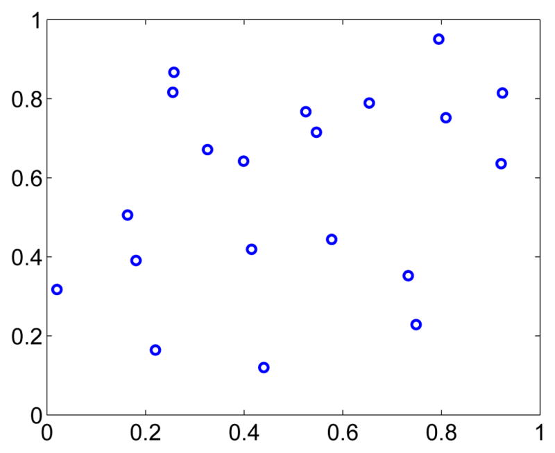
The distribution of nodes in the random geometric graph used in simulation.

Fig. 5.

Time to synchronization for different phase response functions in the identical natural frequency case.

We also simulated the network in the non-identical natural frequency case. The simulation setup is the same as the identical-natural frequency case except that the initial phases were randomly chosen from [0, 2π) and deviations randomly chosen from the interval [−0.01, 0.01] were added to the natural frequencies. The times to frequency synchronization for the three phase response functions under different coupling strengths are given in Fig. 6. It is clear that the optimal phase response function derived in Sec. IV gives a faster rate of frequency synchronization compared with the currently most commonly used phase response functions.

Fig. 6.

Time to synchronization for different phase response functions in the non-identical natural frequency case.

VI. Conclusions

Pulse-coupled synchronization strategies have attracted increased attention in wireless sensor networks. We propose to maximize the synchronization rate by optimizing the phase response function. This can increase the synchronization rate with coupling strengths fixed, and hence can reduce the time to synchronization with the transmission power fixed. Given that the energy consumption is determined by the product of the transmission power and the time to synchronization, the optimal phase response function can reduce energy consumption in synchronization. This has great significance for wireless sensor networks where energy is a valuable system resource.

Biographies

Yongqiang Wang was born in Shandong, China. He received his B.E. degree in Electrical Engineering & Automation, B.E. degree in Computer Science & Technology from Xian Jiaotong University, Shanxi, China, in 2004. From 2007–2008, he was with the University of Duisburg-Essen, Germany, as a visiting student. He received his M.Sc. and Ph.D. degrees in Control Science & Engineering from Tsinghua University, Beijing, China, in 2009. He is now with the University of California, Santa Barbara as a project scientist. His research interests are systems modeling and analysis of biochemical oscillator networks, synchronization of wireless sensor networks, networked control systems, and model-based fault diagnosis.

Dr. Wang is the recipient of 2008 Young Author Prize from IFAC Japan Foundation for a paper presented at the 17th IFAC World Congress in Seoul.

Francis J. Doyle, III received his B.S.E. degree from Princeton in 1985, C.P.G.S. degree from Cambridge in 1986, and Ph.D.degree from Caltech in 1991, all in chemical engineering. He is the Associate Dean for Research in the College of Engineering at UCSB, and he is the Director of the UCSB/MIT/Caltech Institute for Collaborative Biotechnologies. He holds the Duncan and Suzanne Mellichamp Chair in Process Control in the Department of Chemical Engineering as well as appointments in the Electrical Engineering Department and the Biomolecular Science and Engineering Program. He has been awarded the distinction of Fellow in multiple professional societies, including the IEEE, IFAC, AIMBE, and the AAAS. He served as the editor-in-chief of IEEE Transactions on Control Systems Technology from 2004 to 2009 and is the Vice President for Publications in the IEEE Control Systems Society. His research interests are in systems biology, network science, modeling and analysis of circadian rhythms, drug delivery for diabetes, model-based control, and control of particulate processes.

References

- 1.Peskin CS. Mathematical aspects of heart physiology. Courant Institute of Mathematical Science, New York University; New York: 1975. [Google Scholar]
- 2.Mirollo R, Strogatz S. Synchronization of pulse-coupled biological oscillators. SIAM J Appl Math. 1990;50:1645–1662. [Google Scholar]
- 3.Canavier C, Achuthan S. Pulse coupled oscillators and the phase resetting curve. Math Biosci. 2010;226:77–96. doi: 10.1016/j.mbs.2010.05.001. [DOI] [PMC free article] [PubMed] [Google Scholar]
- 4.Mathar R, Mattfeldt J. Pulse-coupled decentral synchronization. SIAM J Appl Math. 1996;56:1094–1106. [Google Scholar]
- 5.Hong YW, Scaglione A. A scalable synchronization protocol for large scale sensor networks and its applications. IEEE J Sel Areas Commun. 2005;23:1085–1099. [Google Scholar]
- 6.Wang YQ, Núñez F, Doyle FJ., III Energy-efficient pulse-coupled synchronization strategy design for wireless sensor networks through reduced idle listening. IEEE Trans Signal Process. doi: 10.1109/TSP.2012.2205685. accepted, 2012. [DOI] [PMC free article] [PubMed] [Google Scholar]
- 7.Werner-Allen G, Tewari G, Patel A, Welsh M, Nagpal R. Firefly inspired sensor network synchronicity with realistic radio effects. Proc. SenSys 05; USA. 2005. pp. 142–153. [Google Scholar]
- 8.Hu A, Servetto SD. On the scalability of cooperative time synchronization in pulse-connected networks. IEEE Trans Inform Theory. 2006;52:2725–2748. [Google Scholar]
- 9.Pagliari R, Scaglione A. Scalable network synchronization with pulse-coupled oscillators. IEEE Trans Mob Comput. 2011;10:392–405. [Google Scholar]
- 10.Konishi K, Kokame H. Synchronization of pulse-coupled oscillators with a refractory period and frequency distribution for a wireless sensor network. Chaos. 2008;18:033132. doi: 10.1063/1.2970103. [DOI] [PubMed] [Google Scholar]
- 11.Okuda T, Konishi K, Hara N. Experimental verfication of synchronization in pulse-coupled oscillators with a refractory period and frequency distribution. Chaos. 2011;21:023105. doi: 10.1063/1.3559135. [DOI] [PubMed] [Google Scholar]
- 12.Izhikevich EM. Dynamical systems in neuroscience: the geometry of excitability and bursting. MIT Press; London: 2007. [Google Scholar]
- 13.Johnson CH. Forty years of PRCs–what have we learned? Chronobiol Int. 1999;16:711–743. doi: 10.3109/07420529909016940. [DOI] [PubMed] [Google Scholar]
- 14.Marella S, Ermentrout GB. Class-II neurons display a higher degree of stochastic synchronization than class-I neurons. Phys Rev E. 2008;77:041918. doi: 10.1103/PhysRevE.77.041918. [DOI] [PubMed] [Google Scholar]
- 15.Hoppensteadt FC, Izhikevich EM. Weakly connected neural networks. Springer; New York: 1997. [Google Scholar]
- 16.Wang YQ, Núñez F, Doyle FJ., III Increasing sync rate of pulse-coupled oscillators via phase response function design: theory and application to wireless networks. IEEE Trans Control Syst Technol. doi: 10.1109/TCST.2012.2205254. accepted, 2012. [DOI] [PMC free article] [PubMed] [Google Scholar]
- 17.Rappaport TS. Wireless communications: principles and practice. Prentice Hall; New York: 2002. [Google Scholar]
- 18.Guckenheimer J, Holmes P. Nonlinear oscillations, dynamical systems and birfurcations of vector fields. Springer-Verlag; New York: 1986. [Google Scholar]
- 19.Vreeswijk CV, Abbott LF, Ermentrout GB. When inhibition not excitation synchronizes neural firing. J Comput Neurosci. 1994;1:313–321. doi: 10.1007/BF00961879. [DOI] [PubMed] [Google Scholar]
- 20.Wang YQ, Doyle FJ., III On influences of global and local cues on the rate of synchronization of oscillator networks. Automatica. 2011;47:1236–1242. doi: 10.1016/j.automatica.2011.01.074. [DOI] [PMC free article] [PubMed] [Google Scholar]
- 21.Brouwer AE, Haemers WH. Spectra of graphs. Springer; New York: 2012. [Google Scholar]
- 22.Mallada E, Tang A. Synchronization of phase-coupled oscillators with arbitrary topology. Proc. American Contr. Conf; Baltimore, USA. 2010. pp. 1777–1782. [Google Scholar]
- 23.Tanenbaum AS. Computer networks. Prentice Hall; New York: 2003. [Google Scholar]
- 24.Strogatz S. From Kuramoto to Crawford: exploring the onset of synchronization in populations of coupled oscillators. Phys D: Nonlin Phenom. 2000;143:1–20. [Google Scholar]
- 25.Varanese N, Spagnolini U, Bar-Ness Y. Distributed frequency-locked loops for wireless networks. IEEE Trans Commun. 2011;59:3440–3451. [Google Scholar]
- 26.Parker P, Mitran P, Bliss D, Tarokh V. On bounds and algorithms for frequency synchronization for collaborative communication systems. IEEE Trans Signal Process. 2008;56:3742–3752. [Google Scholar]