Multi-Organ Segmentation in Abdominal CT Images

Abstract

Automated segmentation of multiple organs in CT data of the upper abdomen is addressed. In order to explicitly incorporate the spatial interrelations among organs, we propose a method for finding and representing the interrelations based on canonical correlation analysis. Furthermore, methods are developed for constructing and utilizing the statistical atlas in which inter-organ constraints are explicitly incorporated to improve accuracy of multi-organ segmentation. The proposed methods were tested to perform segmentation of eight abdominal organs (liver, spleen, kidneys, pancreas, gallbladder, aorta, and inferior vena cava) from various imaging conditions of CT datasets. 87 datasets acquired at two institutions were used for the validation. Significant accuracy improvement was observed for several organs in comparison with the conventional method.

I. INTRODUCTION

In the abdomen, anatomical structures are spatially interrelated. Constraints on the interrelations among the organs as well as individual positions and shapes in the standardized space would be useful to perform their segmentation from 3D images. Several general approaches for multi-organ segmentation have been proposed [1], [2], [3], [4]. Although these works provide unified frameworks for statistical multi-organ modeling and segmentation, the hierarchical nature of organ relations was not explicitly considered. Our assumption is that some organs are constrained in their shapes and locations by other organs whose segmentation is relatively stable and accurate. Such a hierarchical relation can be utilized for effectively constraining the search space to improve the segmentation accuracy and stability. In previous work [5], the hierarchical modeling of multiple organs has been addressed in the pelvic area. However, they tested it for only a small number of organs. More recently, a method for pancreas segmentation was developed by fully utilizing the constraints from surrounding structures [6]. However, the method is not general-purpose but specifically focused on the pancreas.

We developed a general framework of multi-organ segmentation in which hierarchy and interrelations among organs are explicitly incorporated [7]. We also proposed hierarchical statistical atlases based on statistical shape prediction from segmented organs at higher hierarchical levels. Compared with our preliminary work [7], we validated the method using larger number of CT datasets. Further, the hierarchical statistical atlases are constructed in a fully automated manner in this work.

II. METHODS

A. Overview

In this paper, we deal with eight organs, that is, the liver, spleen, left and right kidneys, gallbladder, aorta, inferior vena cava (IVC), and pancreas. The basic idea is to incorporate inter-organ spatial relations to attain stable and accurate segmentation of multiple organs. To do so, we firstly perform segmentation of relatively stable organs in their position, shape, and contrast, and then segment other organs which are expected to be well-constrained in their position and shape by the stable organs segmented during the first step.

We propose a statistical atlas based on shape prediction, which we call prediction-based atlas. Given the segmented interrelated organ regions, the target organ position and shape are predicted from them and the remaining ambiguity is represented in the form of the probabilistic atlas (PA) and statistical shape model (SSM), which we call prediction-based PA and SSM. Prediction-based SSM is combined with multi-level SSM (ML-SSM) where the whole organ shape is hierarchically divided into sub-shapes to attain higher representation accuracy while maintaining the organ-specific shape constraints [8].

B. Basic Method

The basic method is a modified version of a method for liver segmentation using PA and ML-SSM [8]. The modification has been made on modeling the distribution of CT value (which we call “intensity” hereafter) of each organ. While it was originally modeled by a single Gaussian fitted to the patient-specific histogram of the liver in each patient CT dataset estimated from the region having high probability values in PA [8], a Gaussian mixture model is fitted to the average intensity distribution obtained from the training datasets in order to adapt to various organs which may have multi-peak intensity distributions and may be too variable in position to have the high probability region in PA. Because the intensity distribution depends on a contrast enhanced CT protocol, its Gaussian mixture model is assumed to be prepared for each protocol. In constructing ML-SSMs, automated surface subdivision is performed using a significance level of point-pair correlation within the organ surface based on canonical correlation analysis (CCA) [9].

A brief summary of the modified basic method is described below. Given an abdominal CT patient dataset, the abdominal normalized space is determined using the top of the liver dome (determining the height of the reference axial plane) and the bounding box of the bone tissue regions (determining the circumscribed coronal and sagittal planes) as shown in Fig. 1. The liver dome top and bone tissue regions are automatically extracted. The bone tissue regions are extracted by thresholding. The top of the liver dome is extracted by fitting a SSM of the lungs and obtaining their bottom surfaces. They are used to align the patient dataset to the normalized space, in which the PAs and ML-SSMs of all the eight organs are defined. The PA and the intensity model of each organ are used to convert the voxel position and its intensity value to the likelihood of the organ existence, by which the likelihood image is generated. After obtaining the initial region by thresholding the likelihood image, the SSM is fitted to the initial region and then ML-SSM is further fitted to the original CT image to segment the organ region. Finally, a graph-cut-based refinement is performed [10], which was not included in the original basic method [8].

Fig. 1.

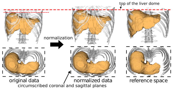
Abdominal normalization using top of live dome and bone tissue regions. The image shows the liver in orange and the ribs and vertebral bodies in white.

C. Organ classification, correlation analysis, and atlas construction

The modified basic method described above was performed for the eight abdominal organs (see Section III for the datasets used for experiments). Based on the segmentation accuracy, we classify them into two categories; stable and variable organs. The Jaccard index (JI) was used as a measure of segmentation accuracy, which is defined by |A∩B|/|A∪B|, where A and B denote the ground truth and automatically segmented region, respectively. If the average JI was significantly larger than 80 %, we regarded it as “stable”, and otherwise “variable”. As a result, the liver and spleen were regarded as “stable”, and the left and right kidneys, gallbladder, aorta, IVC, and pancreas as “variable”. We first segment “stable” organs and then segment “variable” organs assuming that “stable” organs have already been segmented.

In order to find the organ interrelations, CCA is applied. In previous work [9], a p-value to test the significance of correlation between two points was derived using CCA to find intra-organ relations in the brain surface, where small p-values denote strong correlations. We extend this CCA-based method so as to deal with multiple organs. Given organ surfaces X and Y, we define the p-value of point x_i(x_i ∈ X) representing correlation with Y by p_Y(x_i) = min_j p(x_i, y_j), where y_j ∈ Y and p(x, y) is the p-value between points x and y. We define the inter-organ correlation as C(X|Y) = |X_Y|/|X| where $X_Y=\{x_i^{\prime }\mid x_i^{\prime }\in X\wedge p_Y(x_i^{\prime })<\alpha \}$ in which α is the significance level. Intuitively, C(X|Y) denotes a degree of influence of organ Y on organ X. C(X|Y) is not commutative. That is, C(X|Y) ≠ = C(Y|X). For example, when X =“gallbladder” and Y =“liver”, C(X|Y) = 1.0 and C(Y|X) = 0.36 at α = 10⁻²⁴, which means that the whole gallbladder surface is influenced by the liver while 36 % of the liver surface by the gallbladder. Fig. 2(a) shows X_Y of the spleen, left and right kidneys, gallbladder, aorta, IVC, and pancreas when Y =“liver” and α = 10⁻²⁴.

Fig. 2.

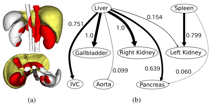
Correlation analysis of inter-organ relations. (a) Organ surfaces influenced by the liver. Yellow surface indicates organ Y (=“liver”). Red indicates the region where $p_Y(x_i^{\prime })<\alpha$. (b) Organ interrelation graph for liver, spleen, left and right kidneys, gallbladder, aorta, IVC, and pancreas.

Based on the classification and correlation analysis, we represent the organ interrelations as a directed graph, which we call the organ interrelation graph (Fig. 2(b)). In the graph, an edge is directed from node Y to node X when Y is a “stable” organ and C(X|Y) is larger than a threshold (the threshold was zero in Fig. 2(b)).

Based on the graph, prediction-based atlases are constructed. For the “variable organs”, prediction-based PA and SSM were constructed based on the prediction from the “stable” organs which have high correlation (represented as arcs in the graph). The prediction-based atlas is described in the next subsection.

D. Prediction-based statistical atlas

The “variable” organ shape v is predicted from the “stable” organs (s = {s₁, s₂, …, s_n−1}) having high correlation with the “variable” organ using partial least squares (PLS) regression [11]. The organ surface shape is assumed to be represented by a point distribution, that is, a vector consisting of the sequence of 3D point coordinates. Let S = (s₁ s₂ … s_N)^t and V = (v₁ v₂ … v_N)^t be the vectors for the “stable” and “variable” organs of the training datasets, respectively, where N is the number of training datasets. Let PLSR(s; S, V) be the regression function of PLS trained using S and V. Given the segmented shape vectors s^* of “stable” organs, the prediction equation is given by v = v^* + r, where v^* = PLSR(s^*; S, V), v is the true shape, and r denotes the residual after the prediction which represents the difference between the predicted and true shapes. Here, r is represented using PA and SSM.

To obtain PA and SSM of r, we consider a reference shape ${\mathbf{v}}_0^{\prime }$ in the reference dataset. The dense 3D deformation field $\mathbf{d}(\mathbf{x};{\mathbf{v}}^{\ast },{\mathbf{v}}_0^{\prime })$ from the original space to the reference space is determined by thin-plate spline interpolation using correspondences from v^* to ${\mathbf{v}}_0^{\prime }$, where x denotes the 3D position in the original space. The correspondences between v^* and ${\mathbf{v}}_0^{\prime }$ are known because they are represented by the same SSM. The true shape v in the original space is mapped to the reference space using $\mathbf{d}(\mathbf{x};{\mathbf{v}}^{\ast },{\mathbf{v}}_0^{\prime })$ and the mapped version v′ is given by ${\mathbf{v}}^{\prime }=\mathbf{v}+\mathbf{d}(\mathbf{x};{\mathbf{v}}^{\ast },{\mathbf{v}}_0^{\prime })$.

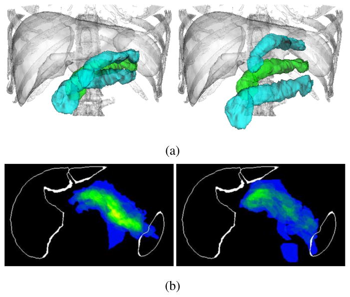
Now, the residual r′ in the reference space is given by ${\mathbf{r}}^{\prime }={\mathbf{v}}^{\prime }-{\mathbf{v}}_0^{\prime }$, which is obtained in each training dataset. In the reference space, SSM and PA of r′ are constructed. The SSM in the reference space is represented as ${\mathbf{q}}^{\prime }({\mathbf{b}}_{\mathrm{r}})={\mathbf{v}}_0^{\prime }+{\mathbf{r}}^{\prime }({\mathbf{b}}_{\mathrm{r}})$, where r′(b_r) = Φ_rb_r, in which Φ_r are the principal components of the residual and b_r their coefficients. The SSM in the original space is obtained by $\mathbf{q}({\mathbf{b}}_{\mathrm{r}})={\mathbf{q}}^{\prime }({\mathbf{b}}_{\mathrm{r}})+{\mathbf{d}}^{-1}({\mathbf{x}}^{\prime };{\mathbf{v}}^{\ast },{\mathbf{v}}_0^{\prime })$, where ${\mathbf{d}}^{-1}({\mathbf{x}}^{\prime };{\mathbf{v}}^{\ast },{\mathbf{v}}_0^{\prime })$ is the inverse deformation filed of $\mathbf{d}(\mathbf{x};{\mathbf{v}}^{\ast },{\mathbf{v}}_0^{\prime })$ and x′ 3D positions in the reference space. The extension of the SSM defined here to ML-SSM is straight forward and it is used for segmentation described in the next section. Similarly, PA is constructing by adding 3D binary images of the true regions v′ in the reference space, and mapped inversely to the original space using ${\mathbf{d}}^{-1}({\mathbf{x}}^{\prime };{\mathbf{v}}^{\ast },{\mathbf{v}}_0^{\prime })$. Fig. 3 shows prediction-based PA and SSM for the pancreas (in comparison with the conventional ones).

Fig. 3.

Constructed prediction-based SSM and PA (left) and those without prediction (right). (a) SSM. (b) PA. In SSM, average (green) and ±2σ (blue) of the first mode are shown. The color-scheme of PA shows probability from cold (low) to hot (high).

E. Segmentation procedure

The additional components which differ from the basic method described in II-B are described. The “stable” organs, the liver and spleen are first segmented. Given segmented “stable” organs, the “variable” organs, right and left kidneys, gallbladder, aorta, IVC, and pancreas, are segmented. Instead of conventional PA and SSM, prediction-based PA and SSM described in II-D are used in the basic method in II-B, followed by ML-SSM fitting and graph-cut refinement.

III. RESULTS

We tested the proposed prediction-based segmentation method using 87 abdominal CT datasets obtained by four different imaging conditions in contrast agent and CT scanner at two hospitals. Table I shows the details of four conditions of CT datasets. In all images, the eight organs (liver, spleen, left and right kidneys, gallbladder, aorta, IVC, and pancreas) were manually segmented by two fellows and supervised by radiologists. However, the aorta and IVC were not segmented for dataset D. Leave-one-out cross validation was performed for evaluation of segmentation accuracy. The intensity model was constructed for each imaging protocol while the same priors on shape and location were utilized for all the datasets. The shape and location models (SSM and PA) were constructed using A, B, and C datasets in Table I. In Fig. 2, if a “variable” organ was related to several “stable” organs, the prediction-based atlas using each of all combinations of the “stable” organs was constructed. That is, for the left kidney and pancreas, which were related to the liver and spleen, the prediction-based atlas using (1) only liver, (2) only spleen, and (3) both liver and spleen were constructed. For other “variable” organs, which were related to the liver, the prediction-based atlases using the liver were constructed.

TABLE I.

Detatils of CT scans used in experiment.

Dataset	Institution	Phase	Number of cases	Number of slices	Slice thickness [mm]
A	Osaka University Hospital	late arterial phase	10	159	2.5
B	Osaka University Hospital	late arterial phase	39	305–409	0.625
C	NIH	venous phase	25	162–291	0.68–1.25
D	NIH	non-contrast	13	250–339	1.0

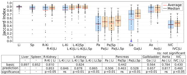
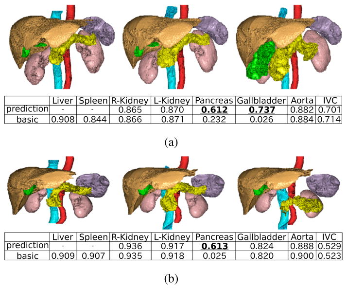
Fig. 4 shows the summary of the segmentation results of the proposed method in comparison with the basic method described in II-B, in which organ interrelations are not explicitly utilized. Fig. 5 shows typical segmentation results. Both methods were fully automated. Segmentation accuracy was evaluated using JI. By using the proposed prediction-based atlases, segmentation accuracy was significantly improved for the left and right kidneys, pancreas, gallbladder, and IVC. Prediction from the spleen only (both the liver and spleen) was most effective for the left kidney (pancreas).

Fig. 4.

Summary of accuracy evaluation of automated abdominal multi-organ segmentation. Average Jaccard index of 87 cases in the proposed prediction-based method (orange box plot) as well as the basic method (blue box plot) for each of eight organs, liver (Li), spleen (Sp), right kidney (R-Ki), left kidney (L-Ki), pancreas (Pa), gallbladder (Ga), aorta (Ao), and IVC, was plotted. Jaccard index values and statistical significance, which was observed for the left and right kidneys, pancreas, gallbladder, and IVC between the proposed prediction-based and basic methods, are also shown below the plots.

Fig. 5.

Manual segmentation (left) and typical segmentation results of proposed (middle) and basic (right) methods. Orange, purple, pink, yellow, green, red, and cyan volumes indicate the liver, spleen, kidneys, pancreas, gallbladder, aorta, and IVC, respectively. Jaccard index of each segmented organ is also shown. JI values of the organs whose segmentation accuracy was particularly improved by the proposed method were enhanced and underlined.

IV. CONCLUSION

This paper has described methods for finding multi-organ spatial interrelations and their incorporation into segmentation via statistical atlas. The methods were applied to the abdominal organs and experimental results showed significant improvement of the segmentation accuracy for the right and left kidneys, gallbladder, IVC, and pancreas. Future work will include adding other abdominal organs and abdominal vessel recognition using segmented organs.

References

- 1.Park H, Bland PH, Meyer CR. Construction of an abdominal probabilistic atlas and its application in segmentation. IEEE Transactions on Medical Imaging. 2003 Apr;22(4):483–492. doi: 10.1109/TMI.2003.809139. [DOI] [PubMed] [Google Scholar]
- 2.Shimizu A, Ohno R, Ikegami T, et al. Segmentation of multiple organs in non-contrast 3D abdominal CT images. International Journal of Computer Assisted Radiology and Surgery. 2007;2(3):135–142. [Google Scholar]
- 3.Linguraru MG, Pura JA, Chowdhury AS, et al. Multi-organ segmentation from multi-phase abdominal CT via 4D graphs using enhancement, shape and location optimization. Medical Image Computing and Computer-Assisted Intervention - MICCAI 2010. 2010;6363:89–96. doi: 10.1007/978-3-642-15711-0_12. ser. LNCS. [DOI] [PMC free article] [PubMed] [Google Scholar]
- 4.Oda M, Nakaoka T, Kitasaka T, et al. Organ segmentation from 3D abdominal CT images based on atlas selection and graph cut. Abdominal Imaging: Computational and Clinical Applications. 2012;7029:181–188. ser. LNCS. [Google Scholar]
- 5.Yokota F, Okada T, Takao M, et al. Automated segmentation of the femur and pelvis from 3D CT data of diseased hip using hierarchical statistical shape model of joint structure. Medical Image Computing and Computer-Assisted Intervention - MICCAI 2009. 2009 Sep;5762:811–818. doi: 10.1007/978-3-642-04271-3_98. ser. LNCS. [DOI] [PubMed] [Google Scholar]
- 6.Shimizu A, Kimoto T, Kobatake H, et al. Automated pancreas segmentation from three-dimensional contrast-enhanced computed tomography. International Journal of Computer Assisted Radiology and Surgery. 2010;5(1):85–98. doi: 10.1007/s11548-009-0384-0. [DOI] [PubMed] [Google Scholar]
- 7.Okada T, Linguraru MG, Yoshida Y, et al. Abdominal multi-organ segmentation of CT images based on hierarchical spatial modeling of organ interrelations. Abdominal Imaging: Computational and Clinical Applications. 2012;7029:173–180. ser. LNCS. [Google Scholar]
- 8.Okada T, Shimada R, Hori M, et al. Automated segmentation of the liver from 3D CT images using probabilistic atlas and multilevel statistical shape model. Academic Radiology. 2008 Nov;15(11):1390–1403. doi: 10.1016/j.acra.2008.07.008. [DOI] [PubMed] [Google Scholar]
- 9.Fillard P, Pennec X, Thompson PM, et al. Evaluating brain anatomical correlations via canonical correlation analysis of sulcal lines. MICCAI 2007 workshop: statistical registration, HAL - CCSD; 2007. [Google Scholar]
- 10.Massoptier L, Casciaro S. Fully automatic liver segmentation through graph-cut technique. Engineering in Medicine and Biology Society, 2007. EMBS 2007. 29th Annual International Conference of the IEEE; August 2007; pp. 5243–5246. [DOI] [PubMed] [Google Scholar]
- 11.Rao A, Aljabar P, Rueckert D. Hierarchical statistical shape analysis and prediction of sub-cortical brain structures. Medical Image Analysis. 2008 Feburary;12(1):55–68. doi: 10.1016/j.media.2007.06.006. [DOI] [PubMed] [Google Scholar]