

Abstract
Accurate prostate segmentation in CT images is a significant yet challenging task for image guided radiotherapy. In this paper, a novel semi-automated prostate segmentation method is presented. Specifically, to segment the prostate in the current treatment image, the physician first takes a few seconds to manually specify the first and last slices of the prostate in the image space. Then, the prostate is segmented automatically by the proposed two steps: (i) The first step of prostate-likelihood estimation to predict the prostate likelihood for each voxel in the current treatment image, aiming to generate the 3-D prostate-likelihood map by the proposed Spatial-COnstrained Transductive LassO (SCOTO); (ii) The second step of multi-atlases based label fusion to generate the final segmentation result by using the prostate shape information obtained from the planning and previous treatment images. The experimental result shows that the proposed method outperforms several state-of-the-art methods on prostate segmentation in a real prostate CT dataset, consisting of 24 patients with 330 images. Moreover, it is also clinically feasible since our method just requires the physician to spend a few seconds on manual specification of the first and last slices of the prostate.
1. Introduction
According to the data [1] reported from National Cancer Institute, prostate cancer will possibly cause 241740 new cases for U.S. male in 2012. It is thus regarded as one of the most leading reasons for cancer-caused death. Recently, CT image guided radiotherapy for prostate cancer treatment has attracted lots of research interest, due to its ability in better guiding the delivery of radiation to prostate cancer [15].
During the CT image guided radiotherapy, a sequence of CT scans will be acquired from a patient in the planning and treatment days. A CT scan acquired in the planning day is called the planning image, and the scans acquired in the subsequent treatment days are called the treatment images. Since the locations of prostate might vary in CT scans, the core problem is to accurately determine the location of prostate in the images acquired from different treatment days, which is usually done by the physician with slice-by-slice manual segmentation. However, manual segmentation can spend a lot of time for each treatment image, i.e., up to 20 minutes. Most importantly, the segmentation results are not consistent across different treatment days due to inter- and intra- operator variability.
The major challenging issues to accurately segment prostate in the CT images include: (i) the boundary between prostate and background is usually unclear due to the low contrast in the CT images, e.g., in Fig.1(a) where the prostate region is highlighted by the physician using green contour. (ii) The locations of the prostate regions scanned at different treatment days are usually different due to the irregular and unpredictable prostate motion, e.g., in Fig.1(b) where the red and blue contours denote the manual segmentations of the two bone-aligned CT images scanned from two different treatment days for the same patient. We can observe the large prostate motion even after bone-based alignment of two scans, indicating the possible large motion of prostate relative to the bones.
Figure 1.

(a) Low contrast in CT image; (b) Large prostate motion relative to the bones, even after bone-based alignment for the two CT images.
Recently, several prostate segmentation methods for CT image guided radiotherapy have been developed, with the common goal of segmenting the prostate in the current treatment image by borrowing the knowledge learned from the planning and previous treatment images. The previous methods can be roughly categorized into three classes: deformable-model-based, registration-based, and learning-based methods. In deformable-model-based methods [6][11], the prostate shapes learned from the planning and previous treatment images are first used to initialize the deformable model, and then specific optimization strategies are developed to guide prostate segmentation. In registration-based methods [7][9][15], the planning and previous treatment images are warped onto the current treatment image, and then their respective segmentation images are similarly warped and further combined (by label fusion) to obtain the final segmentation of the current treatment image. In learning-based methods [14][21], prostate segmentation is first formulated as a prostate-likelihood estimation problem using visual features (e.g., histogram of oriented gradients (HoG) [8] and auto-context features [24]), and then on the obtained likelihood map, the segmentation methods (e.g., level-set segmentation [4]) is adopted to segment the prostate. Note that, besides segmentation on CT images, other prostate segmentation methods are also proposed for segmentation of prostate from other imaging modalities such as MR [12][13] and ultrasound [25] images. Our proposed method belongs to the class of learning-based segmentation methods.
In this paper, we propose a novel prostate segmentation method for CT image guided radiotherapy. Previous learning-based methods [14][21] first collect the voxels from certain slices, and then conduct both the feature selection and the subsequent prostate-likelihood estimation for all voxels in those selected slices jointly. However, different local regions may prefer choosing different features to better discriminate between their own prostate and non-prostate voxels, as indicated by a typical example in Fig.2. In this example, we extracted features for three different local regions, and then apply Lasso (a supervised feature selection technique as introduced in [22]) for the respective feature selections. From the results shown in Fig.2, we can see that the selected features from three local regions are completely different, demonstrating the necessity of selecting respective features for each local region. In this paper, we design a novel local learning strategy: partition each 2-D slice into several non-overlapping local blocks, and then select the respective local features to predict the prostate-likelihood for each local block. This will be achieved by our proposed Spatial-COnstrained Transductive LassO (SCOTO) and support vector regression (SVR), respectively, which will be detailed below. The major difference between the previous learning-based methods and our proposed method can be referred to Fig.3. Note that, before segmentation on the current treatment image, the physician only needs to spend a few seconds to specify just the first and last slices of prostate in the CT image. By spending this little manual time, the segmentation results can be significantly improved, compared with the fully automatic methods [14][15]. The contributions of our proposed method can be summarized into the following two folds:
A novel semi-automatic prostate segmentation method in CT images is proposed. For current treatment image, the information obtained from the planning and previous treatment images of the same patient and also the manual specification of the first and last slices of prostate helps guide the accurate segmentation.
A novel joint feature selection method, called SCOTO, is proposed. SCOTO can successfully select the discriminative features jointly from different local regions (blocks) to guide the better prostate-likelihood estimation.
Figure 2.

A typical examples to illustrate that three different local regions prefer choosing different features. We adopt Lasso as feature selection method, and our used features include LBP, Haar wavelet, and HoG, which will be discussed in the following section.
Figure 3.

The difference between the previous learning-based methods and our proposed method. Our proposed method adopts a local feature selection and prostate-likelihood estimation strategy.
2. Framework, Notation, Image Preprocessing
2.1. Framework
Our proposed method mainly consists of two steps: (i) prostate-likelihood estimation step and (ii) multi-atlases based label fusion step.
In the prostate-likelihood estimation step: First, all previous and current treatment images are rigidly aligned to the planning image of the same patient based on the pelvic bone structures, for removing the whole-body patient motion that is irrelevant to prostate segmentation. Then, we extract the ROI regions according to the prostate center in the planning image. Second, for the current treatment image, physician is required to specify the first and last slices of the prostate in the CT images. By combining the voxels in the specified slices with the voxels sampled from the planning and previous treatment images according to the previous segmentation results, we can extract 2-D low-level features (LBP [20], HoG [8], and Haar wavelet [18]) for all these voxels separately from their original CT images. Then, each 2-D slice will be partitioned into several non-overlapping blocks. The proposed SCOTO is applied for joint feature selection for all blocks, and SVR is further adopted to predict the 2-D prostate-likelihood map for all the voxels in the current slice. Finally, the predicted 2-D prostate-likelihood map of each individual slice will be merged into a 3-D prostate-likelihood map according to the order of their original slices.
In multi-atlases based label fusion step, to make full use of prostate shape information, manually segmented prostate regions in both the planning and the previous treatment images of the same patient will be rigidly aligned to the estimated 3-D prostate-likelihood map of the current treatment image. Then, majority voting will be applied to fuse the labels from different aligned images, and obtain the final segmentation result. The framework of the proposed method is shown in Fig.4.
Figure 4.

The flowchart of the proposed prostate segmentation method.
2.2. Notation
For each patient, we have one planning image, several previous treatment images with their respective manually-refined prostate segmentation results by the physician offline, and also the current treatment image scanned in the current treatment day, which needs to be segmented by the proposed method. The planning image and its corresponding manual segmentation result are denoted as Ip and Gp, respectively. The nth treatment image, which is the current treatment image, is denoted as In. The previous treatment images and their corresponding manual segmentation results are denoted as I1, …, In−1 and G1, …, Gn−1, respectively. Also, the final 3-D prostate-likelihood map and its segmentation result for the current treatment image In by adopting the proposed method are denoted as Mn and Sn, respectively.
2.3. Image Preprocessing
Alignment to the Planning Image
In order to eliminate the influence caused by the whole-body rigid motion which is irrelevant to the prostate motion, we first extract the pelvic bone structure from each image using threshold-based segmentation, and then align each treatment image (I1, …, In) rigidly to the planning image (Ip) based on their pelvic bone structures.
ROI Extraction and Simple Manual Interaction
Basically, the prostates are located only in a small central part of the CT images. So the ROI extraction, which aims to extract the central part by excluding the irrelevant and redundant background voxels, is useful to alleviate the computational burden. For each patient, we first calculate the mass center of the prostate in the planning image Ip, and then extract a large enough 3-D region centered at the calculated mass center. In this paper, the extracted ROI size is 140 × 140 × 60.
When asking physician for manual interaction, we only ask for manual specification of the first and last slices of the prostate along the z-axis. It is noteworthy that the physician’s labeling is done after ROI extraction. Therefore, it will take only less than 10 seconds for this manual step. In the experiments, we will also show that the segmentation results can be largely improved by asking physician to spend such a little interaction time, which is also clinically feasible.
Patch-Based Feature Representation
Three different kinds of features from 2-D slice are extracted, which include 9 histogram of oriented gradient (HoG) [8], 30 local binary pattern (LBP) [20] and 14 multi-resolution Haar wavelet [18]1. The window size for feature extraction is empirically set to 21 × 21. For feature representation, we adopt the patch-based representation method. Specifically, for each voxel, a small patch centered at that voxel with k × k size is used to represent that voxel. The feature vector of the current voxel consists of the features (9+30+14 = 53 features) extracted from all voxels in the small patch. In our paper, the value k is set to 5, so a 1325 (53 × 5 × 5) dimensional feature vector is used to represent each voxel.
Training Voxels Sampling
Because the planning and the previous treatment images with the corresponding manual segmentations are available, voxels with known labels (prostate or background) can be sampled as the training voxels to aid the prostate-likelihood map estimation for the current treatment image. Since the confusing voxels are frequently lying on the boundary of the prostate region, it is reasonable to sample relatively more voxels around the boundary. That is, the boundary voxels will have higher probability to be sampled, as illustrated in Fig.5.
Figure 5.

The typical examples to illustrate the sampling of the training voxels, with the red points denoting the prostate voxels and the blue points denoting the background voxels.
3. Prostate-Likelihood Estimation via SCOTO
3.1. SCOTO: Problem Formulation
For each 2-D slice, our goal is to estimate the prostate-likelihood for each voxel in the current slice. Since our feature representation for each voxel is a high dimensional vector (ℝ1325), the feature selection is significant to avoid the “curse of dimensionality”. For each slice, we first partition the slice into non-overlapping Nx × Ny blocks as shown in Fig.4. Then for the ith block, we use li ∈ ℝ and ui ∈ ℝ to denote the number of training voxels2 and testing voxels, respectively. N ∈ ℝ (N = Nx × Ny) denotes the total number of blocks in the current slice. yi ∈ ℝli+ui and Fi ∈ ℝ(li+ui)×d denotes the ground-truth label and feature matrix for all the training and testing voxels, respectively. Without loss of generality, all the training voxels are listed before the testing voxels in both yi and Fi. d means the number of features (i.e., 1325 in the paper). It is noteworthy that the labels of testing voxels in yi are set to 0. Also in yi, the labels of training voxels are set to 1 if they belong to the prostate, and set to 0 if they belong to the background.
Mathematically, the objective function of SCOTO can be formulated as follows:
| (1) |
where β1, …, βN (βi ∈ ℝd) are the parameters to learn, which indicates the weights of individual features for each block. λS, λL, λE ∈ ℝ are the parameters to control the corresponding terms in Eq.(1), and we will introduce the method for automatic parameter selection in later discussion. Ji ∈ ℝ(li+ui)×(li+ui), which is used to indicate the training voxels since the testing voxels have no contribution on the first term, is a diagonal matrix defined as
is the graph Laplacian with the same definition as that in literature [3]. H(i) denotes the neighbors of the ith block, and |H(i)| is the cardinality of H(i). We use the 4-neighbor connection in this paper.
In Eq.(1), the first term with three sub-terms focuses on each individual block: the 1st sub-term indicates the reconstruction error, the 2nd sub-term imposes the sparsity constraint with L1 norm, and the 3rd sub-term is the graph Laplacian imposing the manifold constraint on both the training and testing voxels since a large amount of testing voxels can be well used for training. The second term of Eq.(1) is the smoothness term on the neighboring blocks, so that the neighboring blocks can choose similar features. Therefore, Eq.(1) can be considered as the derivation from Lasso [22] by imposing manifold constraint and spatial smoothness over neighboring blocks.
3.2. Optimization
To solve Eq.(1), since the feature weight vectors β1, …, βN are jointly convex, the alternating optimization method [17] can be employed, which sequentially solves βi with other variables βj (1 ≤ j ≤ N, j ≠ i) fixed. Therefore, the optimization for Eq.(1) can be divided into several alternating sub-problems. Formally, for each βi, when fixing the other parameters βj, we have the following sub-problem:
| (2) |
The problem of Eq.(2) is convex but not smooth for the feature weight vector βi, so the closed-form solution cannot be reached. For solving Eq.(2), we consider adopting the iterative projected gradient descent method [2] for optimization, which separates the sub-problem into the smooth term and the non-smooth term, and solves them iteratively until convergence. Therefore, the Eq.(2) can be separated into the smooth term
and the non-smooth term N (βi) = λS∥βi∥1.
The iterative projected gradient descent method contains two steps in each iteration. For the kth iteration, in the first step, we compute using Newton gradient descent method as
| (3) |
where γk ∈ ℝ is the step size which can be automatically determined by the back-tracking line search for each iteration. and denote the 1st and 2nd order derivatives of S(βi) at respectively, which can be calculated as follows:
and
where Ĵi = JiJi ∈ ℝ(li+ui)×(li+ui). Qi ∈ ℝ(li+ui)×d is defined as for clear representation.
In the second step, with the obtained α(k), we update to by solving the following L1 regularized regression problem:
| (4) |
The Eq.(4) can be efficiently solved by many existing algorithms, e.g., LARS [10].
The algorithm summary for SCOTO can be referred to Algorithm 1. The input is the feature matrices and the corresponding labels of individual blocks, and the output is the corresponding feature weights for each block.
Algorithm 1 SCOTO
Input: feature matrices F1,…,FN, and the corresponding labels y1,…,yN.
Output: feature weights β1,…,βN.
1: for i ← 1, …, N do
2: Li ← calculate the graph Laplacian [3].
3: ← solution by applying Lasso on Fi and yi.
4: end for
5: k ← 1
6: while not converge do
7: for i ← 1, …, N do
8: ← solution by Eq.(3).
9: ← solution by Eq.(4).
10: end for
11: end while
After SCOTO for feature selection, for the ith block, the features, which correspond to the entries in βi that are larger than 0, will be selected. So we can finally obtain the new feature matrices (i = 1, …, N) by selecting the columns in Fi corresponding to the selected features.
3.3. Prostate-Likelihood Estimation
With the obtained new feature matrices (i = 1, …, N), we can estimate the prostate-likelihood for each block. For each individual block, we apply SVR, which is a conventional regression method, to predict the prostate-likelihood for all the voxels in each block. Specifically, SVR model is first trained by the training voxels in as well as available labels in yi, and then preformed over the ui testing voxels on the ith block for prediction of prostate. All the predicted likelihood will be finally normalized into [0, 1]. It is noteworthy that we will first obtain 2-D prostate-likelihood maps slice by slice, and then merge all the results to get the final 3-D prostate-likelihood map, which is denoted as Mn.
4. Multi-Atlases based Label Fusion
To make full use of all the shape information from the planning and previous treatment images for segmentation, we adopt the multi-atlases based label fusion with the following steps: First, previous binary segmentation results G1,…,Gn−1 and Gp will be rigidly aligned to estimated prostate-likelihood map Mn by using the mutualinformation based similarity metric with Powell’s optimization strategy; Second, we average all the obtained aligned results and conduct the voxel-wise majority voting to get the final segmentation result Sn, which can be referred to the “multi-atlases based label fusion” step in Fig.4.
5. Experimental Results
5.1. Dataset Description and Experimental Setup
The proposed method is evaluated on a prostate 3-D CT-image dataset consisting of 24 patients with 330 images, and each patient has at least 9 images obtained from 1 planning day and several treatment days. The original resolution of each image is 512 × 512 × 60, with in-plane voxel size as 0.98 × 0.98 mm2 and the inter-slice thickness as 3 mm. All the images of the patients are manually segmented by experienced physician, which are used as ground-truth for evaluation in the experiments. For each patient, the first 3 images (i.e., the planning image and the first two treatment images) are used as training images, from which the training voxels are sampled, and segmentation ground-truths are available.
In the experiments, we use three common evaluation metrics: the Dice ratio, the true positive fraction (TPF), and the centroid distance (CD). Specifically, the Dice ratio between two binary images A and B can be calculated as 2|A∩B|/(|A|+|B|). The TPF indicates that the percentage of corrected predicted prostate voxels in the manually segmented prostate regions. The centroid distance means the Euclidean distance between the central locations of the manual segmentation result and predicted result. Since prostate CT-images are 3-D, the CD along 3 directions, including the lateral (x-axis), anterior-posterior (y-axis), and superior-inferior (z-axis) directions, need to be calculated. Note that, in the superior-inferior (z-axis) direction, the CD is calculated as 3 times of the obtained value since the inter-slice voxel size is 3 mm, which is approximately 3 times of that in the x-axis and y-axis.
5.2. Parameter Selection
For the parameter selection in SCOTO, λS, λL, λE are automatically selected by grid searching with leave-one-out cross-validation on three patient-specific training images. It is noteworthy that the parameters in SVR, which is implemented by LIBSVM toolbox [5], are set to default ones. The λS, λL, λE with the best results are selected, and we found λS = 10−6, λL = 10−8, λE = 10−3 to be best. For the size of blocks, we empirically set to 10 (note that the slice size after ROI extraction is 140 × 140). Too large block size will ignore the variations of appearance along the prostate boundary, while too small block size will increase the computational burden. However, it is still an open problem on how to automatically choose block size, which we will study in our future work.
5.3. Evaluation on the SCOTO
To evaluate the SCOTO on feature selection and also to validate if the block-level feature selection is better than the slice-level feature selection, we introduce several related feature selection methods for comparison, which include LassoS and tLassoS (applying Lasso [22] and tLasso [21] on slice-level feature selection, respectively), LassoB and tLassoB (applying Lasso and tLasso on block-level feature selection, respectively), mRMR [19] and fused Lasso [23]. For all these methods, the parameters are experimentally set using leave-one-out cross-validation. It is noteworthy that the same multi-atlases based label fusion is adopted for all the methods.
Table.1 lists the segmentation accuracies obtained by different feature selection schemes, and the best results are marked by the bold fonts. We found SCOTO can achieve superior performance over the related methods. Specifically, we also found that (i) the block-level methods are better than the slice-level ones, which validates our assumption that different local regions prefer choosing different features; (ii) Manifold constraint is useful for improving the results (by comparing tLassoS with LassoS, and tLassoB with LassoB); (iii) Spatial-constraint smoothness term leads to better results (by comparing SCOTO with tLassoB).
Table 1.
Comparison of experimental results among different feature selection methods, with the best results marked by bold font.
| level | methods | Dice (mean ± std) | TPF (mean ± std) | CD (mean ± std) (x/y/z) (mm) |
|---|---|---|---|---|
| image-level feature selection | LassoS | 0.874 ± 0.083 | 0.869 ± 0.107 | 0.71 ± 0.56 / 0.80 ± 0.61 / 0.67 ± 0.53 |
| tLassoS | 0.917 ± 0.053 | 0.899 ± 0.084 | 0.54 ± 0.37 / 0.50 ± 0.38 / 0.40 ± 0.33 | |
| block-level feature selection | mRMR | 0.893 ± 0.033 | 0.912 ± 0.047 | 0.50 ± 0.34 / 0.72 ± 0.41 / 0.36 ± 0.33 |
| LassoB | 0.922 ± 0.039 | 0.909 ± 0.042 | 0.47 ± 0.39 / 0.47 ± 0.37 / 0.33 ± 0.34 | |
| tLassoB | 0.932 ± 0.036 | 0.919 ± 0.040 | 0.37 ± 0.17 / 0.41 ± 0.35 / 0.32 ± 0.33 | |
| fused Lasso | 0.928 ± 0.047 | 0.906 ± 0.043 | 0.34 ± 0.37 / 0.42 ± 0.38 / 0.34 ± 0.51 | |
| SCOTO | 0.941 ± 0.030 | 0.924 ± 0.037 | 0.25 ± 0.18 /0.30 ± 0.22 / 0.27 ± 0.29 |
5.4. Comparison with Previous Methods
To further evaluate the performance of the proposed method, the results of several state-of-the-art methods are illustrated for comparison, which include deformable-model based methods [6][11], registration-based methods [9][15], and learning-based method [14][21]. The best results reported in the corresponding papers are listed. The comparisons among different methods are listed in Table 2. Evaluated metrics include mean Dice ratio and median TPF (Note that, in [6][14], median TPF are evaluated instead of mean TPF). Because different CT datasets are used for experiments in Davis et al.’s work [9] and Chen et al.’s work [6], the results are listed separately for reference. For [11][15][21], all the 24 patients are evaluated, which is the same with ours, so we name the 24 patients CT dataset as “CT dataset 1”. Also, two different subsets of the 24 patients are selected in [14] and [15], which are named as “CT dataset 2” and “CT dataset 3”, respectively. From the results listed in Table 2, we can find that the proposed method outperforms the related methods in terms of higher mean Dice ratio and median TPF. In addition, the mean average surface error of our method is 1.09mm, which is better than 2.37mm (reported in [16]) and 2.47mm (reported in [11]).
Table 2.
The results of mean Dice ratio and median TPF, compared with the related methods, with the best results marked by bold font.
| PAs | IMs | methods | mean Dice | median TPF | |
|---|---|---|---|---|---|
| Other datasets | 3 | 40 | Davis et al.[9] | 0.820 | N/A |
| 13 | 185 | Chen et al.[6] | N/A | 0.840 | |
| CT dataset 1 | 24 | 330 | Feng et al.[11] | 0.893 | N/A |
| Liao et al.[15] | 0.899 | N/A | |||
| Shi et al.[21] | 0.920 | 0.901 | |||
| our method | 0.941 | 0.932 | |||
| CT dataset 2 | 11 | 164 | Li et al.[14] | 0.908 | 0.900 |
| Shi et al.[21] | 0.923 | 0.911 | |||
| our method | 0.940 | 0.923 | |||
| CT dataset 3 | 10 | 176 | Liao et al.[15] | 0.896 | N/A |
| Shi et al.[21] | 0.922 | 0.907 | |||
| our method | 0.936 | 0.923 |
Moreover, we report the patient-specific results of Dice ratio and TPF in Fig.6, and CDs in Fig.7 for each individual patient. For statistical perspective, quartile-representation is adopted, in which five horizontal lines (ascending order in values) mean the min, 25% percentile, median, 75% percentile, and the max value, respectively.
Figure 6.

The results of Dice ratio and TPF for 24 patients.
Figure 7.
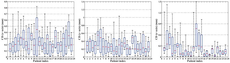
The results of CD along the lateral (x-axis), anterior-posterior (y-axis), and superior-inferior (z-axis) directions, respectively.
Finally, we also illustrate in Fig.8 several typical segmented examples as well as prostate-likelihood map for the image 14 of patient 3, the image 10 of patient 11, the image 5 of patient 16, the image 6 of patient 21 and the image 8 of patient 24, respectively. In Fig.8, the red curves denote the manual segmentation results by the physician, and the yellow curves denote the segmentation results by the proposed methods. We found that the predicted prostate boundaries are very close to the boundaries delineated by the physician. Also the proposed method can accurately separate the prostate regions and background even in the base and apex slices as shown in Figs.8(a)8(d), which are usually considered very difficult to segment.
Figure 8.

Typical segmentation results and prostate-likelihood maps for Patients 3, 11, 16, 21, 24. Red curves indicate manual segmentation results by physician and the yellow curves indicate the segmentation results by our proposed method.
5.5. Patients with Large Prostate Motion
In our work, it is found that the patients 3, 10 and 15 have larger prostate motions according to the standard deviation of prostate centers in the planning and treatment images, which can be found by referring to Fig.9. By applying the proposed method to patients 3, 10 and 15, the obtained median Dice ratio are 0.909, 0.928, and 0.946, respectively, which are better than the corresponding results reported in [14][21]. These comparisons are also listed in Fig.10. These results show the effectiveness of the proposed method, especially with the initial physician’s manual interaction when the large irregular motion occurs in the prostate regions.
Figure 9.

The standard deviation of prostate centers for each patients.
Figure 10.
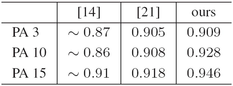
The median Dice ratios for Patient 3, 10, 15, with large prostate motion.
6. Conclusion
We have proposed a novel semi-automatic learning method for prostate segmentation in CT images during the image-guided radiotherapy. Our proposed SCOTO will first jointly select the discriminative features for the individual local image regions, for helping generate the prostate-likelihood map. Then, the multi-atlases based label fusion method will combine the segmentation results of the planning and previous treatment images for final segmentation. A real CT-prostate dataset is used for evaluation, which consists of 24 patients and 330 images, all with the manual delineation results by the experienced physician. Experimental results show that our proposed method not only obtains superior segmentation performance (i.e., higher Dice ratio and TPF, and lower centroid distances) compared with the state-of-the-art methods, but also demonstrates its capability in dealing with large irregular prostate motions.
Acknowledgments
the work is support by the National Science Foundation of China (Nos. 61035003, 61175042, 61021062), the National 973 Program of China (No. 2009CB320702), the 973 Program of Jiangsu, China (No. BK2011005), Program for New Century Excellent Talents in University (No. NCET-10-0476) and Jiangsu Clinical Medicine Special Program (No. BL2013033). The work is also supported by the grant from National Institute of Health (No. 1R01 CA140413).
Footnotes
HOG: calculated within 3×3 cell blocks with 9 histogram bins similar in [8]. LBP: calculated with radius value 2 and neighboring voxel number 8. Haar: calculated by convolving the 14 multi-resolution wavelet basis functions with the input image similar in [18].
The training voxels come from the sampled voxels, whose locations are in the current block within the slices [sc −1, sc +1] of training images, where sc is the current slice index of testing voxels in z-axis. The reason is that training voxels in adjacent slices have similar distribution in feature space, which guarantees enough voxels are sampled, especially on the base and apex slices of prostate.
References
- 1.Prostate Cancer, report from National Cancer Institute. link: http://www.cancer.gov/cancertopics/types/prostate.
- 2.Beck A, Teboulle M. A fast iterative shrinkage-thresholding algorithm for linear inverse problems. SIAM J Img Sci. 2009;2(1):183–202. [Google Scholar]
- 3.Belkin M, Niyogi P, Sindhwani V. Manifold regularization: a geometric framework for learning from labeled and unlabeled examples. JMLR. 2006;7:2399–2434. [Google Scholar]
- 4.Chan T, Esedoglu S, Nikolov M. Algorithms for finding global minimizers of image segmentation and denoising models. SIAM Journal on Applied Mathematics. 2006;66:1632–1648. [Google Scholar]
- 5.Chang C-C, Lin C-J. Libsvm : a library for support vector machines. ACM TIST. 2011;2:1–27. [Google Scholar]
- 6.Chen S, Lovelock D, Radke R. Segmenting the prostate and rectum in CT imagery using anatomical constraints. Medical Image Analysis. 2011;15:1–11. doi: 10.1016/j.media.2010.06.004. [DOI] [PubMed] [Google Scholar]
- 7.Chen T, Kim S, Zhou J, Metaxas D, Rajagopal G, Yue N. 3D meshless prostate segmentation and registration in image guided radiotherapy. MICCAI. 2009:43–50. doi: 10.1007/978-3-642-04268-3_6. [DOI] [PubMed] [Google Scholar]
- 8.Dalal N, Triggs B. Histograms of oriented gradients for human detection. CVPR. 2005:886–893. [Google Scholar]
- 9.Davis B, Foskey M, Rosenman J, Goyal L, Chang S, Joshi S. Automatic segmentation of intra-treatment CT images for adaptive radiation therapy of the prostate. MICCAI. 2005:442–450. doi: 10.1007/11566465_55. [DOI] [PubMed] [Google Scholar]
- 10.Efron B, Johnstone I, Hastie T, Tibshirani R. Least angle regression. Annals of Statistics. 2003;32:407–499. [Google Scholar]
- 11.Feng Q, Foskey M, Chen W, Shen D. Segmenting CT prostate images using population and patient-specific statistics for radiotherapy. Medical Physics. 2010;37:4121–4132. doi: 10.1118/1.3464799. [DOI] [PMC free article] [PubMed] [Google Scholar]
- 12.Gao Y, Sandhu R, Fichtinger G, Tannenbaum A. A coupled global registration and segmentation framework with application to magnetic resonance prostate imagery. IEEE TMI. 2010;29:1781–1794. doi: 10.1109/TMI.2010.2052065. [DOI] [PMC free article] [PubMed] [Google Scholar]
- 13.Langerak T, et al. Label fusion in atlas-based segmentation using a selective and iterative method for performance level estimation (SIMPLE) IEEE TMI. 2010;29:2000–2008. doi: 10.1109/TMI.2010.2057442. [DOI] [PubMed] [Google Scholar]
- 14.Li W, Liao S, Feng Q, Chen W, Shen D. Learning image context for segmentation of prostate in CT-guided radiotherapy. MICCAI. 2011:570–578. doi: 10.1007/978-3-642-23626-6_70. [DOI] [PMC free article] [PubMed] [Google Scholar]
- 15.Liao S, Shen D. A feature based learning framework for accurate prostate localization in CT images. IEEE TIP. 2012;21:3546–3559. doi: 10.1109/TIP.2012.2194296. [DOI] [PubMed] [Google Scholar]
- 16.Lu C, Zheng Y, Birkbeck N, Zhang J, Kohlberger T, Tietjen C, Boettger T, Duncan J, Zhou S. Precise segmentation of multiple organs in ct volumes using learning-based approach and information theory. MICCAI. 2012:462–469. doi: 10.1007/978-3-642-33418-4_57. [DOI] [PubMed] [Google Scholar]
- 17.Luo Z, Tseng P. On the convergence of the coordinate descent method for convex differentiable minimization. Journal of Optimization Theory and Applications. 1992;72(1):7–35. [Google Scholar]
- 18.Mallat G. A theory for multiresolution signal decomposition: the wavelet representation. IEEE TPAMI. 1989;11:674–693. [Google Scholar]
- 19.Mallat G. Feature selection based on mutual information: criteria of max-dependency, max-relevance, and min-redundancy. IEEE TPAMI. 2005;27:1226–1238. doi: 10.1109/TPAMI.2005.159. [DOI] [PubMed] [Google Scholar]
- 20.Ojala T, Pietikainen M, Maenpaa T. Multiresolution gray-scale and rotation invariant texture classification with local binary patterns. IEEE TPAMI. 2002;24:971–987. [Google Scholar]
- 21.Shi Y, et al. Transductive prostate segmentation for CT image guided radiotherapy. MICCAI workshop: Machine Learning in Medical Imaging; 2012. pp. 1–9. [Google Scholar]
- 22.Tibshirani R. Regression shrinkage and selection via the lasso. JRSSB. 1996;58:267–288. [Google Scholar]
- 23.Tibshirani R, Saunders M, Rosset S, Zhu J, Knight K. Sparsity and smoothness via the fused lasso. JRSSB. 2005;67:91–108. [Google Scholar]
- 24.Tu Z, Bai X. Auto-context and its application to high-level vision tasks and 3D brain image segmentation. IEEE TPAMI. 2010;32:1744–1757. doi: 10.1109/TPAMI.2009.186. [DOI] [PubMed] [Google Scholar]
- 25.Zhan Y, et al. Targeted prostate biopsy using statistical image analysis. IEEE TMI. 2007;26:779–788. doi: 10.1109/TMI.2006.891497. [DOI] [PubMed] [Google Scholar]