Abstract
Diffusion-weighted imaging (DWI), while giving rich information about brain circuitry, is often limited by insufficient spatial resolution and low signal-to-noise ratio (SNR). This paper describes an algorithm that will increase the resolution of DW images beyond the scan resolution, allowing for a closer investigation of fiber structures and more accurate assessment of brain connectivity. The algorithm is capable of generating a dense vector-valued field, consisting of diffusion data associated with the full set of diffusion-sensitizing gradients. The fundamental premise is that, to best preserve information, interpolation should always be performed along axonal fibers. To achieve this, at each spatial location, we probe neighboring voxels in various directions to gather diffusion information for data interpolation. Based on the fiber orientation distribution function (ODF), directions that are more likely to be traversed by fibers will be given greater weights during interpolation and vice versa. This ensures that data interpolation is only contributed by diffusion data coming from fibers that are aligned with a specific direction. This approach respects local fiber structures and prevents blurring resulting from averaging of data from significantly misaligned fibers. Evaluations suggest that this algorithm yields results with significantly less blocking artifacts, greater smoothness in anatomical structures, and markedly improved structural visibility.
Keywords: Diffusion Magnetic Resonance Imaging (DMRI), Resolution Enhancement, Anisotropic Interpolation
1. Introduction
Diffusion magnetic resonance imaging (DMRI) (Johansen-Berg and Behrens, 2009) is a key imaging technique for the investigation and characterization of white matter pathways in the brain. It probes water diffusion in various directions and at various diffusion scales to characterize micro-structural compartments that are much smaller than the voxel size. However, limited by today’s imaging technique, the typical (2mm)3 resolution achievable by DMRI is too coarse to sufficiently capture the subtlety of neuronal axons, diameters of which range from 1 μm to 30 μm (Johansen-Berg and Behrens, 2009; Scherrer et al., 2012; Yap and Shen, 2012a). This causes significant partial volume effect since the signal collected at each voxel is likely to be due to multiple fascicles that concurrently traverse the voxel. Acquiring images with resolution higher than the typical (2mm)3, however, is extremely difficult without incurring unrealistic scan times and causing very low SNR due to reduced voxel size (Scherrer et al., 2012). The impact of noise is aggravated in high angular resolution diffusion imaging (HARDI), which often requires prolonged echo time (TE) to achieve relatively high diffusion weighting.
Increasing the resolution is not only important for registration, segmentation, and tractography to be performed with greater accuracy, but is also crucial for better visualization of anatomical structures to identify possible neuropathologies. Solutions to achieve higher resolution include employing higher magnetic fields or stronger/faster gradients, dedicated acquisition techniques (Liu et al., 2004; Scherrer et al., 2012; Heidemann et al., 2012; Sotiropoulos et al., 2013), as well as post-processing algorithms (Nedjati-Gilani et al., 2008; Calamante et al., 2010; Manjóon et al., 2010a; Gupta et al., 2013). In the current work, we will take the post-processing approach, since this approach does not rely on expensive scanner upgrades and complex time-consuming sequences and can hence be applied to existing data without requiring re-acquisition.
In this paper, we present a technique that will exploit the continuity information given by local fiber architectures to increase the spatial resolution of diffusion-weighted data beyond the acquisition resolution. Our algorithm will generate a spatially dense vector-valued field consisting of diffusion data associated with the full set of diffusion-sensitizing gradient directions. Similar to (Calamante et al., 2010), our approach gains spatial resolution by using additional information obtained from outside each individual voxel. Dissimilar to (Nedjati-Gilani et al., 2008; Gupta et al., 2013), our method does not assume any diffusion model and is applied directly to the DW images. Our approach does not require special acquisition techniques, such as those proposed in (Greenspan et al., 2002; Greenspan, 2009; Scherrer et al., 2012), does not need expensive scanner hardware upgrades (to 7T or 11T), and can be applied to existing data. The key highlights of our method is as follows:
Directional Profiling — Our approach uses a directional profiling scheme to examine the neighborhood of each spatial location and to gauge the probability of whether a specific direction is likely to be traversed by fibers. The resulting directional probability distribution is then employed to encourage interpolation along tangential and not orthogonal directions of axonal fibers. Unlike the conventional trilinear interpolation, which does not take into account the directional nature of DWI data, our approach mimics DWI acquisition mechanism more closely by borrowing information from different directions to reconstruct the DWI data at each spatial location.
Microstructure-Preserving Smoothing — DWI data are typically noisy and need to be smoothed for increasing SNR. When smoothing, it is important that boundaries defining the spatial extent of individual structures are preserved. In contrast to many existing methods that use inter-voxel gradient information to constrain smoothing to relatively homogeneous regions, our method uses intra-voxel fiber orientation distribution functions (ODFs) to guide smoothing. By constraining interpolation along fiber streamlines, we not only preserve boundaries of the white matter, but also those between fiber tracts within the white matter.
Complete DWI Data — Our approach generates a vector-valued field of DWI data corresponding to the full set of diffusion-gradients and is not limited to the white matter. Gray matter provides contextual information for the white matter and the availability of gray matter data allows tissue segmentation based on diffusion data, such as that done in (Liu et al., 2007), to be performed, providing complementary tissue contrast to tissue segmentation based on structural MRI. The fact that our method produces a complete set of DWI data also allows any diffusion models to be fitted to the resolution-enhanced data for multifaceted analysis.
A preliminary version of this work was presented in (Yap and Shen, 2012a).
1.1. Paper Organization
In the upcoming sections, we will first detail in Section 2 the key components of the proposed algorithm. We will then demonstrate the effectiveness of the proposed algorithm in Section 3 with both in silico and in vivo data. Additional discussion is provided in Section 4 before the paper is concluded in Section 5.
2. Material and Methods
2.1. Datasets
Various datasets were acquired or generated for comprehensive evaluation of the proposed method. They are described as follows.
2.1.1. In Silico Data
To quantitatively evaluate the accuracy of the proposed method, we generated a 96 × 96 field of diffusion-weighted signal, forming a spiral as shown in Fig. 2(A). Each voxel within the spiral was simulated using a tensor model with principal diffusivities λ1 = 1.5×10⁻³ mm2/s, λ2 = λ3 = 3×10⁻⁴ mm2/s, and diffusion weighting b = 2,000 s/mm2. The baseline non-diffusion-weighted signal S0 was set to 150. Diffusion-weighted signal was sampled along each of the 120 gradient directions obtained from the in vivo dataset (see Section 2.1.2). The background voxels that fall outside the spiral were generated via isotropic diffusion with constant signal magnitude S0 exp(−bλ), where b = 2,000 s/mm2, λ = 2.5 × 10⁻³ mm2/s, and S0 = 1,000. Note that these diffusion parameters were carefully chosen to mimic the in vivo dataset described in Section 2.1.2.
Figure 2. Synthetic Data.
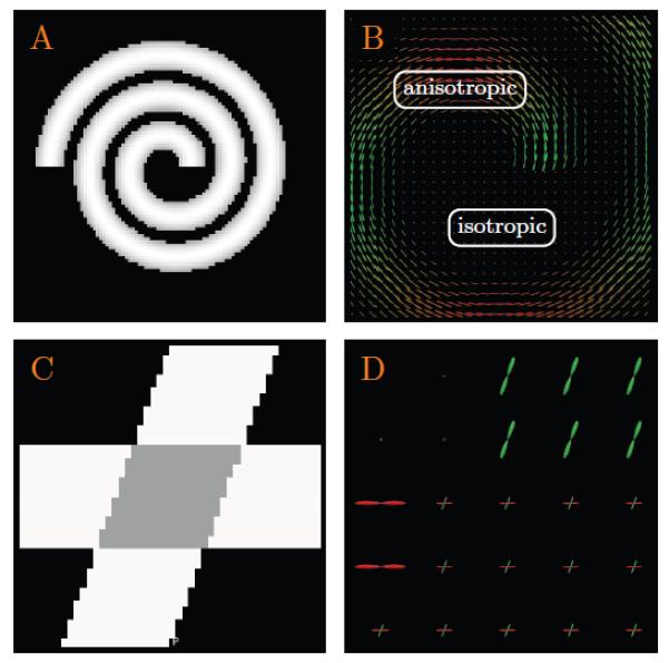
(A) The spiral and (C) the cross (only the case of 60° is shown here) used for evaluation. The left panels (A) & (C) show the anisotropy maps and the right panels (B) & (D) show the close-up views of the respective ODF fields.
2.1.2. In Vivo Data
Diffusion-weighted images for 4 adult subjects were acquired using a Siemens 3T TIM Trio MR scanner with an EPI sequence. Diffusion gradients were applied in 120 non-collinear directions with diffusion weighting b = 2,000 s/mm2, repetition time (TR) = 12,400ms, and echo time (TE) = 116ms. The imaging matrix was 128 × 128 with a field of view (FOV) of 256 × 256mm2. The slice thickness was 2mm. Six non-diffusion-sensitized images (b = 0 s/mm2) were acquired. T1-weighted structural images with 1mm isotropic resolution were also acquired as anatomical references.
2.1.3. High-Resolution In Vivo Data
For further evaluation, a set of high-resolution (1mm)3 diffusion-weighted images were acquired using the Siemens 3T TIM Trio MR scanner with the acquisition technique reported in (Porter and Heidemann, 2009). Diffusion gradients were applied in 42 non-collinear directions with diffusion weighting b = 1,000 s/mm2. The imaging matrix was 192 × 192 with a field of view of 192 × 192mm2. The slice thickness was 1mm.
2.1.4. Neonatal Data
Diffusion-weighted images of a neonate were acquired at approximately one month after birth. Diffusion gradients were applied in 42 non-collinear directions with diffusion weighting b = 1,000 s/mm2, TR = 7,680ms and TE = 82ms. The scans covered the whole brain with a resolution of 2×2×2mm3.
2.2. Fiber-Driven Resolution Enhancement
To increase spatial resolution, the image domain is uniformly divided using a grid with grid elements that are smaller than the acquisition voxel size. The diffusion-weighted data for each of these grid elements are then generated using the following steps: 1) Directional profiling in a field of fiber ODFs; 2) Interpolation of diffusion-weighted data based on the fiber orientation profile (generated in the previous step) with bias correction (owing to the Rician distribution nature of the magnitude signal), and 3) Mean-shift refinement for recovering more structural details. Each step is detailed in the following sections.
2.2.1. Local Fiber Profiling
Interpolation along directions transversed by fibers preserve structural boundaries. To determine the probability of whether a grid element at spatial location x is traversed by fibers in directions vk (k = 1, … , M), which are densely distributed on the unit sphere and not necessarily antipodal symmetric, we profile for each k the field of fiber ODFs {p(xi, v)|xi ∈ N (x)} along direction v = vk (see Fig. 1), where N(x) is a neighborhood of voxels in the vicinity of x. Note that xi is a point in space at which the diffusion-weighted signal is actually acquired, and x is a point corresponding to a grid element of a high-resolution grid, using which the resolution-enhanced data will be reconstructed. The local fiber configuration at x is characterized by a fiber orientation profile, which is a directional function that allows for anisotropic interpolation of neighboring information to generate the DWI data of the grid element at location x. It is determined as
| (1) |
where
| (2) |
The weighted are defined as
| (3) |
if daxial > 0 or 0 otherwise. Here daxial and dradial are respectively the (signed) axial distance (length parallel to the reference line) and the radial distance (length perpendicular to the reference line), as illustrated in Fig. 1. Specifically,
| (4) |
and
| (5) |
where || · || is the Euclidean norm.
Figure 1. Directional Profiling.
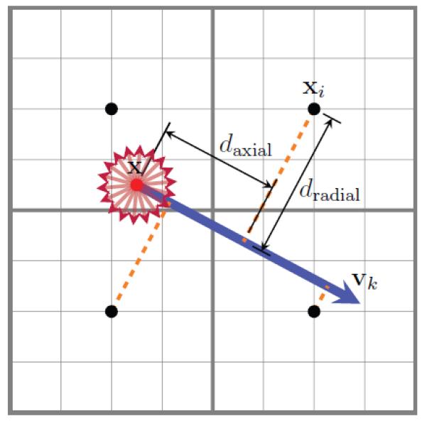
The space resided by the voxels (black dots) are divided by a grid using a resolution that is finer than the acquisition resolution (a factor of 4 in each dimension). For each grid element of interest (red dot), we probe its neighborhood in directions vk, k = 1, … , M (red arrows) to obtain a fiber orientation profile p̂(x, vk), which is essentially a directional function informing us of the certainty of interpolating along a certain direction. The location x and direction vk define a reference line (blue). Voxels closer to the reference line, measured with daxial(xi, x, vk) and dradial(xi, x, vk), will be given greater weights during interpolation.
Parameters σaxial and σradial control the falloff of the weight with respect to the axial and radial distances, respectively. They are determined heuristically as follows. By setting the full width at half maximum (FWHM) of the radial term to one voxel, the value of σradial can be computed as
| (6) |
Determining σaxial is less straightforward. We want to determine the distance to profile in the axial direction so that the assumption of local linearity reasonably holds. For an angle θ off the axial direction and a distance r along the axial direction, the deviation distance from the axial direction can be determined as
| (7) |
Setting Δ to one voxel and r to half of the FWHM of the axial term, i.e., we have
| (8) |
In the present work, we set θ = π/6 (= 30°), resulting in σaxial = 1.622 and σradial = 0.425.
2.2.2. Fiber-Sensitive Interpolation With Rician-Bias Correction
The fiber orientation profile at location x gives an indication of which directions are most likely to be traversed by fibers. The diffusion-weighted data of voxels in the neighborhood of x should therefore be weighted according to the fiber orientation profile — directions that are more likely to be traversed by fibers should be given greater weights. To generate the data at location x, we compute
| (9) |
where gl for l = 1, 2, … , N correspond to the directions of the diffusion-sensitizing gradients,
| (10) |
and
| (11) |
is the weighted mean of the squared diffusion-attenuated signal S2(·, ·) in direction vk. Note that the squared signal values are used here so that the statistical bias can be removed for unbiased estimation. This is derived from the fact that the second order moment of a Rician distributed quantity is given as (Gudbjartsson and Patz, 1995)
| (12) |
where Strue is the true signal value. The noise variance associated with the Rician distribution (Nowak, 1999) can be estimated from the background signal (Strue = 0) using . To account for spatially non-uniform noise level, adaptive methods such as that proposed in (Manjóon et al., 2010b) can be used for voxel-wise estimation of σrician.
2.2.3. Mean-Shift Refinement
When generating the data for a particular voxel, essentially a mean is computed based on the weighted averaging of neighboring data. However, despite our effort up to this point to determine appropriate weights for the neighboring voxels based on spatioangular information, it is still possible that voxels with diffusion-weighted signal that are significantly different from voxels in the neighborhood are included in the averaging process, causing unnecessary variability in the estimation. This problem can be mitigated by refining the mean using a mean-shift mechanism (Fukunaga and Hostetler, 1975; Cheng, 1995). More specifically, the mean can be refined iteratively by considering its similarity with the signal values of neighboring voxels, determining a set of radiometrically-modulated weights, and then computing a new mean. In order to achieve this, we note that (9) can be rewritten as
| (13) |
where
| (14) |
The vector Ŝ2(x, gl) is in fact the minimizer of the weighted sum of squared distances from an arbitrary squared signal vector a(gl) to each squared signal vector S2(xi, gl) at point xi with weight ρ(xi, x). That is,
| (15) |
The mean of the squared signal S̄2(x, gl) can be refined iteratively by rewriting the equation as
| (16) |
where the variable t is introduced here to denote the iteration. Note that here we modulate the weight with radiometric similarity by defining
| (17) |
which degenerates to ρi(x) when σradiometric is large:
| (18) |
The parameter is estimated adaptively as
| (19) |
where | · | denotes the cardinality of a set. The iteration stops when the difference between the means estimated in two subsequent iterations falls below a pre-specified threshold or when a certain number of iterations is reached.
3. Results
In this section, the results for the evaluation of the proposed DWI resolution enhancement method using in silico and in vivo data (see Section 2.1) are reported. For all cases, we set σaxial = 1.622 and σradial = 0.425, as discussed in Section 2.2.1. Directional profiling was performed in 642 directions, which were generated by subdividing the faces of an icosahedron 3 times. The fiber ODF field was computed by fitting mixtures of tensors to the diffusion-weighted data. An over-complete set of tensors were used and the fitting problem was solved using a non-negative L1-constrained sparse representation framework (Yap and Shen, 2012b). ODFs computed using other approaches (Aganj et al., 2010; Descoteaux et al., 2007; Tournier et al., 2007) can also be used in the proposed resolution-enhancement framework. We chose to utilize the method described above because it produces sharp ODFs that are helpful for better preservation of structures when up-sampling the data.
3.1. In Silico Data
The spiral data (see Section 2.1.1) were down-sampled by factors of 2 and 4 by averaging every 4 voxels and every 16 voxels, respectively. Rician noise of different levels was then added to the down-sampled data before they were up-sampled using the proposed method for evaluation using the original data as ground truth. The performance metric used for measuring up-sampling accuracy was the root-mean-square error (RMSE). This evaluation was performed 10 times for each noise level.
For the signal at each voxel location and gradient direction, the Rician noise corrupted signal S̃ was computed as (Coupóe et al., 2008)
| (20) |
where n1 and n2 are sampled from normal distributions with zero mean and variance . The value S̃ is a realization of a Rician-PDF random variable with parameters S and σrician.
Results for noise levels σrician = 0, 2, 4, 6, 8 are shown in Fig. 3. σrician = 4 corresponds approximately to the noise level of the in vivo data. We compared our method with
A modified form of vector-based trilinear interpolation, where each element of the signal vector was squared and interpolated using trilinear interpolation, followed by the removal of the Rician bias and a square root operation (refer (13)).
Anisotropic interpolation with no mean-shift refinement (i.e., by setting σradiometric → ∞ in (17)).
Figure 3. Spiral Data.
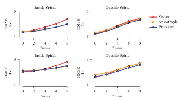
The average RMSE values with respect to different levels of Rician noise. The standard deviations are negligible. Results for vector-based trilinear interpolation, anisotropic interpolation, and the proposed method are shown for voxels inside the spiral (anisotropic) and outside the spiral (isotropic).
It can be observed from the figure that the proposed method yields significantly improved up-sampling accuracy when compared to vector-based trilinear interpolation both for the voxel within the spiral, i.e. the anisotropic voxels, and voxels outside the spiral, i.e., the isotropic voxels. The proposed method also, in overall, performs better than anisotropic interpolation. Incorporating the additional mean-shift mechanism brings further improvement by allowing certain degree of non-linearity in the course of interpolation to cope better with situations where fibers are not exactly locally linear.
A ‘cross’ phantom, shown in Fig. 2(C), was also used to evaluate the proposed method in situations where fiber crossings exist. Using the same diffusion parameters described above for the spiral, we used diffusion tensors and their mixtures to generate a phantom of size 48 × 48 for evaluation. One group of tensors were oriented in the horizontal direction and another group at an angle, i.e., 30°, 40°, … , 90°, with the horizontal direction. At locations where these two groups cross, a mixture of two tensors with equal volume fraction was used to model the crossings. The results, shown in Fig. 4, indicate that our method yields results with lesser error for most cases at different noise levels and different crossing angles.
Figure 4. Cross Data.
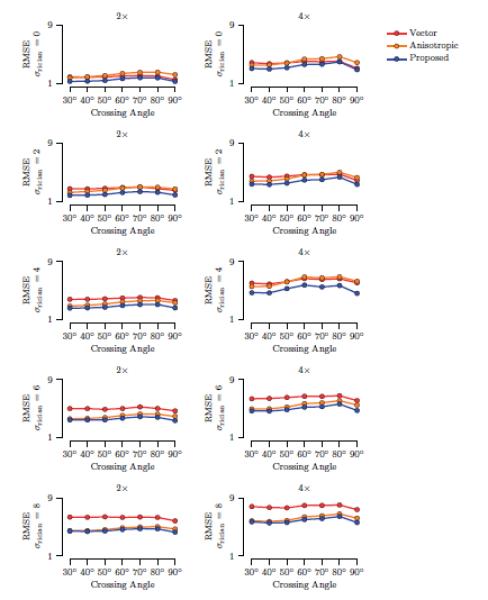
The average RMSE values, computed over the anisotropic region, with respect to different levels of Rician noise and different angles of crossing. The standard deviations are negligible. Results for factors 2 and 4 are shown.
In subsequent experiments, we will focus on the comparison between the proposed method and vector-based trilinear interpolation.
3.2. In Vivo Data
In this section, we report the results for the evaluation of the proposed method using the in vivo diffusion-weighted data described in Section 2.1.2.
3.2.1. Evaluation Method
We up-sampled each DW image from its original resolution of (2mm)3 to (0.5mm)3. Results generated by trilinear interpolation, performed both on the anisotropy map as well as the vector-valued diffusion-weighted data, were used for comparison. The generalized anisotropy at each voxel location was computed as the standard deviation to RMS ratio of the signal values, i.e.,
| (21) |
3.2.2. Qualitative Evaluation
A set of representative results are shown in Fig. 5, with close-up views provided in Fig. 6. It is clear from the results that the proposed method yields results that exhibit significantly less blocking artifacts, greater smoothness in anatomical structures, and markedly improved structural visibility. Note that interpolation of diffusion-weighted data benefits quite significantly from interpolation schemes that consider the directionality of the data. From the figure we can see that when interpolation is performed on the scalar anisotropy image, the resulting image is blurred with not much structural details. Details are however much more readily visible when interpolation is performed on the vector-valued diffusion-weighted data, i.e., by independently interpolating each element of the data vector across space. This is largely due to the fact that by doing so we are essentially computing a convex combination of neighboring diffusion data that is associated with each particular gradient direction. While clearly giving more structural details, vector-based trilinear interpolation results in significant blockiness due to the Cartesian nature of the interpolation. All these problems are effectively dealt with using the proposed method, as is evident from the results.
Figure 5. DWI Resolution Enhancement.
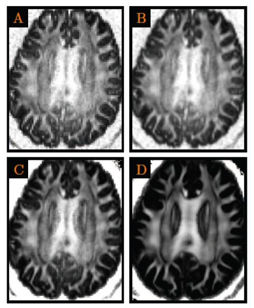
DW images were up-sampled to a (0.5mm)3 resolution from the original (2mm)3 resolution. (A) The anisotropy image of the original data; (B) The linearly up-sampled anisotropy image (i.e., scalar interpolation); (C) The anisotropy image of the linearly up-sampled DWI data; and (D) The anisotropy image given by the proposed method. Close-up views are shown in Fig. 6.
Figure 6. Close-Up Views.
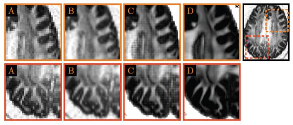
Regional close-up views of Fig. 5.
Fig. 7 shows representative results for an individual diffusion-weighted image associated with a single gradient direction. It can be observed that noise is effectively smoothed out without destroying structural boundaries. Note that the gradient direction for this example is approximately in the left-right direction. Therefore, white matter structures with fibers running in the left-right direction should have a darker intensity due to the greater signal attenuation owing to diffusion; white matter structures with fibers running in the anterior-posterior direction (or superior-inferior direction) should have brighter intensity due to lesser attenuation.
Figure 7. Representative Results for a Diffusion-Weighted Image.
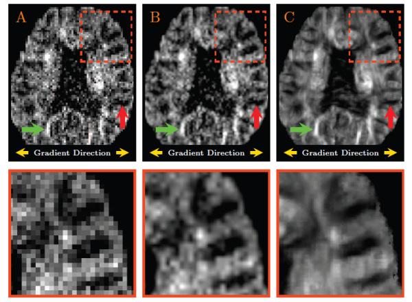
(A) A diffusion-weighted image in the original resolution; (B) The linearly up-sampled image; and (C) The up-sampled image generated with the help of the directional information borrowed from the diffusion-weighted data. Since the gradient direction for this example is approximately in the left-right direction, white matter structures with fibers running in the left-right direction should have a darker intensity (see for example the structure marked by the red arrow); white matter structures with fibers running in the anterior-posterior direction or superior-inferior direction should have brighter intensity (see for example the structure marked by the green arrow).
To assure that the orientational information of the up-sampled data is consistent with the underlying anatomy, we show in Fig. 8 close-up views of the ODF field generated from the up-sampled data. The T1-weighted image is also provided for reference. The local fiber orientations indicate that the orientational information is correctly preserved in relation to the white matter structures.
Figure 8. ODF Fields.
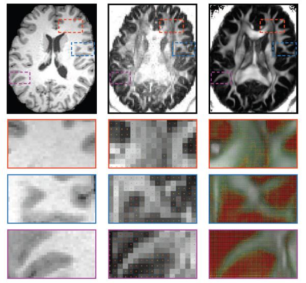
Close-up views of the ODF fields of the original data (middle) and the up-sampled data (right). The corresponding anatomical T1-weighted image (left) is provide for reference.
In Fig. 9, we show how the various components of the proposed method help to improve the final outcome. The images in the figure show that interpolation with an isotropically extended voxel neighborhood helps improve the SNR of the image but blurs the structures. The result can be improved by taking into consideration the anisotropic nature of the structures. The mean-shift refinement mechanism helps improving the result further.
Figure 9. Reconstruction Refinement.
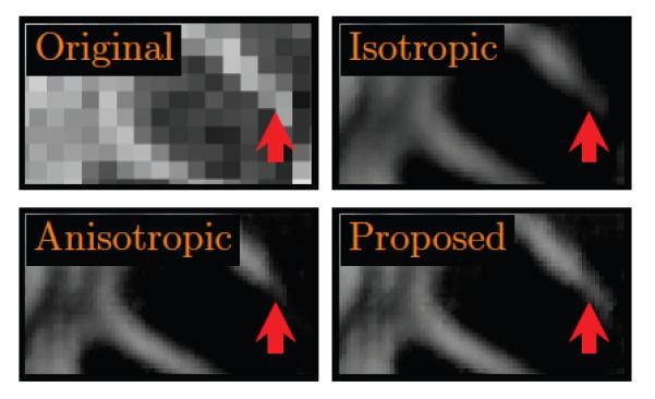
The various components of the proposed method helps refine the final outcome. The result for isotropic interpolation was generated by setting p̂(x, vk) = 1. The result for anisotropic interpolation was generated by setting σradiometric → ∞. Without mean-shift refinement, the white matter structure marked by the red arrow is lost.
3.2.3. Quantitative Evaluation
For quantitative evaluation, we computed the local variances of the generalized anisotropy values in the white matter (WM), gray matter (GM) and cerebrospinal fluid (CSF). For this purpose, we segmented the T1-weighted image associated with each of the 4 subjects into WM, GM, and CSF. These segmented images were then used as masks to compute the average anisotropy variances for regions corresponding to WM, GM, and CSF. The variability of the anisotropy values gives us an indication on how smooth the interpolated image is. The results, shown in Fig. 10, indicate that the proposed method, while giving markedly improved structural details, as shown in the previous section, also yields greater structural smoothness. Such smoothness is important for applications such as tractography to ensure that fiber pathways can be traced more reliably with greater continuity.
Figure 10. Average Regional Variance of Generalized Anisotropy.
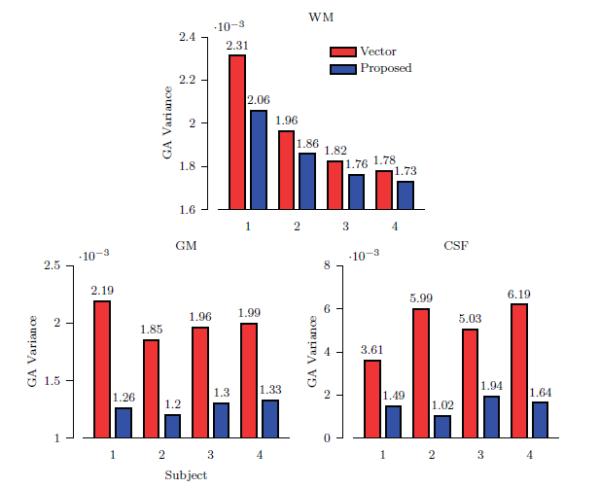
The anisotropy variance at each voxel location is computed using a 3 × 3 × 3 neighborhood. The bars show the average values of the anisotropy variance. Only results for vector-based linear interpolation and the proposed method are shown since these two methods yield better structural clarity.
We performed further evaluation by examining the consistency between the resolution enhanced data and the respective T1-weighted images. Here, we leveraged the fact that T1-weighted images are acquired at a resolution that is typically twice higher than that of diffusion-weighted scans. Comparing the resolution enhanced data with the T1-weighted images provides an indicator of whether the resolution enhancement process produces spurious structures that do not actually exist. To carry out this evaluation, we first labeled the WM, GM, and CSF regions obtained from the T1-weighted images with values 1, 0, and 0, respectively. These values were chosen to match the observation that on an anisotropy image the white matter (WM) voxels show the brightest values (closer to 1) owing to diffusion anisotropy resulting from restricted diffusion; this is followed by the gray matter (GM) voxels, which generally exhibit a lower degree of anisotropy, and then the cerebrospinal fluid (CSF) voxels, which exhibit isotropic diffusion. To simplify the evaluation, we made the assumption that GM and CSF voxels are totally isotropic and label these regions in the T1-weighted images with zero.
Linearly up-sampling the value-labeled images to match the resolution of the resolution enhanced data, we evaluated the resolution enhancement consistency by computing
| (22) |
where A(x) and L(x) are respectively the anisotropy and label value at voxel location x. Ω denotes the brain region. ϕ ranges from 0 to 1, corresponding to low to high consistency. Fig. 11 shows the consistency values for direct scalar interpolation of the anisotropy images of the original diffusion-weighted data, vector-based interpolation, and the proposed method over subjects. The results validate that the proposed method produces results with greater anatomical accuracy.
Figure 11. Anatomical Consistency.
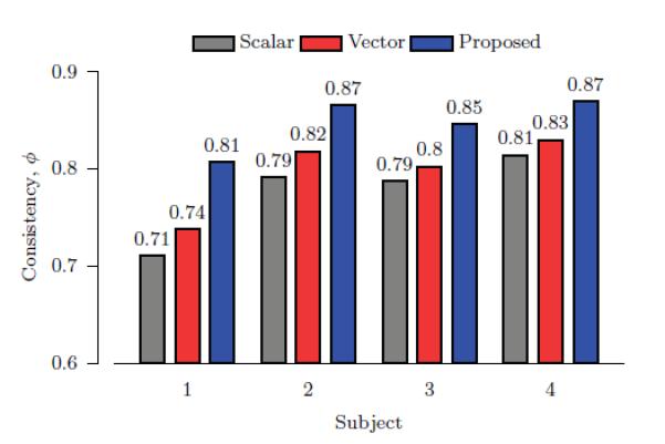
Anatomical accuracy of the resolution enhanced data is evaluated with the help of value-labeled WM, GM, and CSF segmentations of respective T1-weighted images.
3.3. Visual Evaluation Using High-Resolution Data
We down-sampled the high resolution data (see Section 2.1.3) by averaging every eight voxels. The proposed algorithm was then applied to this down-sampled data to generate the resolution-enhanced data with resolution (1mm)3. The results, shown in Fig. 12, indicate that our method is able to generate realistic resolution-enhanced data that greatly resembles the data acquired at high resolution. This implies that, in situation where the luxury of scanning in high resolution is not practical, our algorithm can be used as an alternative means for post-processing-based resolution enhancement.
Figure 12. Evaluation Using High-Resolution Data.
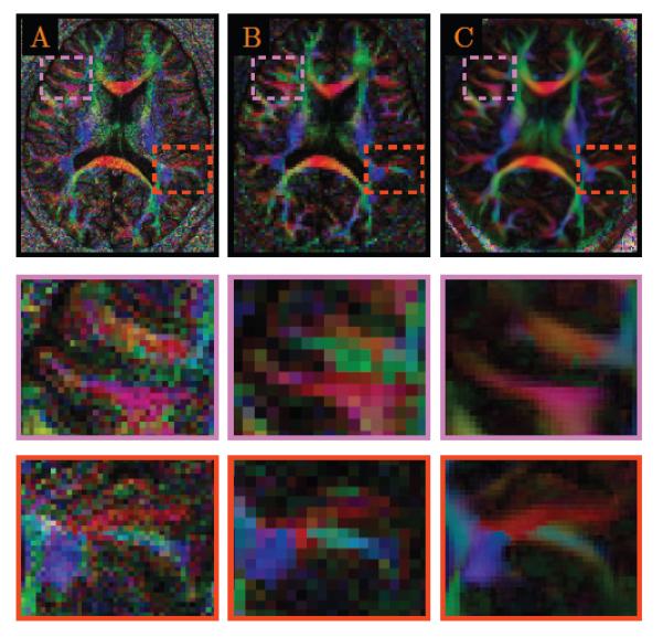
Color-coded fractional anisotropy images of the (A) original data at (1mm)3, (B) down-sampled data at (2mm)3, and (C) resolution-enhanced data at (1mm)3. Close-up views are shown in the two bottom rows.
3.4. Application to Neonatal Data
The resolution problem of DWI is aggravated in the case of neonates because the average brain size of babies at birth is less than half of that of the adult (Knickmeyer et al., 2008). In this section, we demonstrate that significant improvement in spatial resolution of neonatal data (see Section 2.1.4) can be achieved using our method.
3.4.1. Structural Clarity
We evaluated whether our method could improve the structural clarity of the neonatal DWI data. Consistent with the results shown previously, Fig. 13 shows that resolution enhancement to (0.5mm)3 using our method gives markedly improved structural clarity over the data in the original resolution. The zoomed insets indicate that cortical structures, which are often barely visible in diffusion scans of neonatal subjects, can now be clearly visible.
Figure 13. Resolution Enhancement of Neonatal DWI Data.
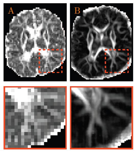
(A) Anisotropy image of the original data; and (B) The anisotropy image of the resolution enhanced data generated using the proposed method.
3.4.2. Tractography
To evaluate whether resolution enhancement improves tractography, we tracked and compared a number of well-studied major fiber bundles, i.e., the forceps minor, the forceps major, the uncinate fasciculus, and the cingulum bundle using the original data and the resolution enhanced data generated with our method.
Whole brain probabilistic streamline fiber tractography was first performed and the relevant fiber bundles were then extracted using regions of interest placed as described in (Wakana et al., 2007). The local fiber orientations were determined based on the fiber ODF at each voxel location (Yap and Shen, 2012b). At locations where multiple orientations exist, one orientation (subject to turning angle less than 40°) was randomly selected. Fiber tracing was initiated using seeds randomly subsampled within voxels with anisotropy greater than 0.10. For the data in the original resolution, seed subsampling was performed (2.0/0.5)3 = 64 times more than that performed for the resolution enhanced data to compensate for the difference in the number of voxels within a specified region. Fiber tracing was carried out with a step size of 0.5mm and was stopped when a voxel with anisotropy less than 0.05 was encountered or when the turning angle was greater than 40°. The motivation for a low anisotropy value allowance was so that the tracing could proceed into unmyelinated white matter regions.
Fig. 14 shows that the forceps major, the forceps minor, the uncinate fasciculus, and the cingulum bundle can be tracked with greater success using the resolution enhanced data. The resolution enhanced data give fuller and more complete fiber tracts that are in greater agreement with our anatomical understanding of the fibers. This improvement in estimating the neuronal trajectories is of paramount importance for connectivity-based neuro-developmental studies involving neonatal subjects.
Figure 14. Effects of Resolution Enhancement on Tractography.
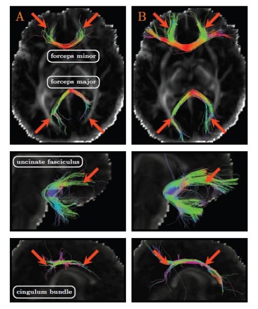
(A) Tractography using the original data; and (B) Tractography using the resolution enhanced data generated using the proposed method.
3.5. Computation Time
We implemented the proposed method using the Insight Segmentation and Registration Toolkit (ITK)1 and most of our ITK filters allow multithreading. Using the in vivo data described in Section 2.1.2 as an example and assuming that the fiber ODFs have been pre-computed, approximately 100 s is required to generate a high-resolution (0.5mm)2 slice for all 120 gradient directions using a MacBook Pro with a 2.6 GHz Intel Core i7 processor.
4. Discussion
This work leverages local fiber directional information for effective interpolation of diffusion-weighted data, reducing image blur that often accompanies image up-sampling. This is done by gathering information from neighboring, anatomically connected voxels to inform the estimation of the data at each voxel. This provides a powerful mechanism that will allow us to collapse measurements across multiple voxels to estimate micro-structural parameters shared along a single fiber bundle and improve estimation dramatically.
Track-density imaging (TDI) was proposed by Calamante et al. (2010) to super-resolve diffusion data. TDI gains its image contrast by computing the number of fiber streamlines traversing each element of a high-resolution image grid. In order to generate a super-resolution image, whole-brain probabilistic tractography is first performed (generated by randomly seeding a large number of tracts throughout the brain, e.g., >1,000,000). From these fiber tracts, the total number of tracts traversing each grid element is then calculated. Essentially, TDI is leveraging fiber continuity (Reisert and Kiselev, 2011) to super-resolve each voxel. While promising, TDI is limited for the following reasons: 1) The results can only be as accurate as the tractography algorithm employed; 2) Contrast can only be extracted from regions that can be reached by the fiber streamlines (i.e., regions with reasonably high diffusion anisotropy); and 3) Only scalar maps, computed from fiber statistics, can be generated. All these problems can be avoided by using the proposed approach.
Experiments on synthetic data have shown that the proposed method yields significant improvement over the commonly used vector-based trilinear interpolation. We note here however, at regions where the fibers bend sharply, there is an increase in the reconstruction error. This is understandably so since the proposed algorithm relies on the local linearity of fibers, an assumption which might not hold perfectly in real-world scenarios. The effect of the deviation of the fibers from being locally linear is shown in Fig. 15. It can be observed that the error is greater for voxels closer to the center of the spiral where the curvature is higher. In future, this issue can be addressed by utilizing locally adaptive parameters, an approach that is quite common in image processing.
Figure 15. Effect of Fiber Curvature.
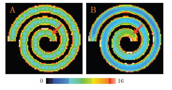
The average RMSE images, at noise level σrician = 8, for (A) vector-based trilinear interpolation and (B) the proposed method. While the proposed method generally results in lower error, the RMSE value increases for voxels closer to the center of the spiral center (marked by the red arrows), where the fiber curvature is greater. Background voxels were masked off for the sake of clarity.
Note that the proposed method does not attempt to disentangle the contributions of the fiber populations that traverse each voxel and, when performing interpolation, assigns a single weight to each neighboring voxel irrespective of the diffusion-sensitizing gradient direction. This may introduce blurring of the diffusion signal at locations where the fiber geometry changes spatially, e.g., when transitioning from a voxel with no crossing to one with crossing. In (Yap et al., 2013), we have attempted to deal with such problem by proposing a different approach that decomposes the diffusion signal spatially and angularly in the position-orientation space (POS) for improved super-resolution of diffusion data. White matter connectivity information is used to regularize this otherwise ill-posed inverse problem. The interested reader is referred to (Yap et al., 2013) for more details.
Evaluation using real data is less straightforward since we do not have the ground truth but only noisy signal observations. Fortunately, we were able to use anatomical information from T1-weighted images, prior knowledge on fiber configurations, prior knowledge on anisotropy image contrast in relation to different tissue types, and high-resolution data to show that the proposed method indeed yields results that are closer to our expectations about the brain.
We have also investigated the effectiveness of interpolation using higher order methods such Lanczos interpolation and B-spline interpolation. The results from these methods, shown in Fig. 16, indicate that these higher-order methods suffer from similar blocking artifacts as vector-based trilinear interpolation. The blocking artifact is due to the noisy nature of the data. When used to interpolate values between the sampling points (with actual signal measurements), these methods yield lower generalized anisotropy values because the interpolated values are computed based on the weighted averages of the measurements at the sampling points, suppressing some noise and at the same time decreasing the anisotropy. However, at the sampling points themselves, no significant averaging is carried out since these methods tend to assign to these points the actual measured values. Since these measured values are noisy, the generalized anisotropy values tend to be higher due to the greater perceived anisotropy stemming from the greater standard deviation of the signal values [refer (21)]. The combination of the brighter voxels with higher anisotropy and darker voxels with lower anisotropy voxels causes the blockiness. Given the greater flexibility of these higher-order interpolation methods, they might be susceptible to the effect of noise, and might not necessarily perform better than lower-order methods.
Figure 16. Higher-Order Interpolation.

Comparison of A) the proposed method and B) vector-based trilinear interpolation with C) Lanczos interpolation, D) third-order B-spline interpolation, and E) fourth-order B-spline interpolation.
Clinical studies on neurological disorders, especially those involving white matter, can benefit from the resolution-enhanced data. For example, the increased structural clarity of the resolution enhanced data might be helpful for more accurate differentiation of acute from chronic multiple sclerosis plaques (da Cruz Jr et al., 2011). At systems level, the better tractography results given by our method, as shown in Fig. 14, is helpful for studying the brain connectome (Yap et al., 2010) in relation to growth (Yap et al., 2011a) and disorders (Shi et al., 2012; Wee et al., 2011, 2012). Our algorithm is especially important for enhancing the resolution of pediatric scans, which are normally very poor in terms of spatial resolution due to the relatively smaller brain size. This is aggravated by the fact that tractography on pediatric data is known to be especially difficult and error-prone (Yap et al., 2011c,b), hampering connectivity analysis to be carried out accurately. The improvement yielded by our method is hence important for studies involving target groups such as children.
5. Conclusions
In conclusion, we have presented a technique for effective up-sampling of DWI data, producing results that are free from blocking artifacts and imaging noise while at the same time show excellent structural clarity. Our work prompts the need of a closer examination on the effect of interpolation artifacts on the performance of various DWI algorithms, such as tractography. Future work will be directed at utilizing locally non-linear interpolation strategies to elucidate even finer structural details and to resolve complex fiber configurations, such as branching and kissing.
Highlights.
We present in this work an effective method for up-sampling diffusion-weighted images by using the rich connection architecture of white matter. Our method
Produces results that are free from blocking artifacts and imaging noise while at same time gives excellent structural clarity.
Produces resolution enhanced data for all diffusion directions as well as all tissue types.
Allows the myriad of existing diffusion models to be fitted on the resolution-enhanced diffusion data for multifaceted analysis.
Acknowledgment
This work was supported in part by a UNC start-up fund and NIH grants (EB006733, EB008374, EB009634, MH088520, AG041721, and MH100217).
Footnotes
Publisher's Disclaimer: This is a PDF file of an unedited manuscript that has been accepted for publication. As a service to our customers we are providing this early version of the manuscript. The manuscript will undergo copyediting, typesetting, and review of the resulting proof before it is published in its final citable form. Please note that during the production process errors may be discovered which could affect the content, and all legal disclaimers that apply to the journal pertain.
References
- Aganj I, Lenglet C, Sapiro G, Yacoub E, Ugurbil K, Harel N. Reconstruction of the orientation distribution function in single- and multiple-shell q-ball imaging within constant solid angle. Magnetic Resonance in Medicine. 2010;64:554–566. doi: 10.1002/mrm.22365. [DOI] [PMC free article] [PubMed] [Google Scholar]
- Calamante F, Tournier J, Jackson G, Connelly A. Track-density imaging (TDI): Super-resolution white matter imaging using whole-brain track-density mapping. Neuroimage. 2010;53:1233–1243. doi: 10.1016/j.neuroimage.2010.07.024. [DOI] [PubMed] [Google Scholar]
- Cheng Y. Mean shift, mode seeking, and clustering. IEEE Transactions on Pattern Analysis and Machine Intelligence. 1995;17:790–799. [Google Scholar]
- Coupóe P, Yger P, Prima S, Hellier P, Kervrann C, Barillot C. An optimized blockwise nonlocal means denoising filter for 3-D magnetic resonance images. IEEE Transaction on Medical Imaging. 2008;27 doi: 10.1109/TMI.2007.906087. [DOI] [PMC free article] [PubMed] [Google Scholar]
- da Cruz LCH, Jr, Batista RR, Domingues RC, Barkhof F. Diffusion magnetic resonance imaging in multiple sclerosis. Neuroimaging Clinics of North America. 2011;21:71–88. doi: 10.1016/j.nic.2011.02.006. [DOI] [PubMed] [Google Scholar]
- Descoteaux M, Angelino E, Fitzgibbons S, Deriche R. Regularized, fast, and robust analytical q-ball imaging. Magnetic Resonance in Medicine. 2007;58:497–510. doi: 10.1002/mrm.21277. [DOI] [PubMed] [Google Scholar]
- Fukunaga K, Hostetler LD. The estimation of the gradient of a density function, with applications in pattern recognition. IEEE Transaction on Information Theory. 1975;IT-21:32–40. [Google Scholar]
- Greenspan H. Super-resolution in medical imaging. The Computer Journal. 2009;52:43–63. [Google Scholar]
- Greenspan H, Oz G, Kiryati N, Peled S. MRI inter-slice reconstruction using super-resolution. Magnetic Resonance Imaging. 2002;20:437–446. doi: 10.1016/s0730-725x(02)00511-8. [DOI] [PubMed] [Google Scholar]
- Gudbjartsson H, Patz S. The Rician distribution of noisy MRI data. Magnetic Resonance in Medicince. 1995;34:910–914. doi: 10.1002/mrm.1910340618. [DOI] [PMC free article] [PubMed] [Google Scholar]
- Gupta V, Ayache N, Pennec X. Improving DTI resolution from a single clinical acquisition: A statistical approach using spatial prior, in: Medical Image Computing and Computer-Assisted Intervention (MIC-CAI) 2013. [DOI] [PubMed]
- Heidemann RM, Anwander A, Feiweier T, Knöosche TR, Turner R. k-space and q-space: combining ultra-high spatial and angular resolution in diffusion imaging using ZOOPPA at 7 T. NeuroImage. 2012;60:967–78. doi: 10.1016/j.neuroimage.2011.12.081. [DOI] [PubMed] [Google Scholar]
- Johansen-Berg H, Behrens TE, editors. Diffusion MRI — From Quantitative Measurement to In vivo Neuroanatomy. Elsevier; 2009. [Google Scholar]
- Knickmeyer RC, Gouttard S, Kang C, Evans D, Wilber K, Smith JK, Hamer RM, Lin W, Gerig G, Gilmore JH. A structural mri study of human brain development from birth to 2 years. The Journal of Neuroscience. 2008;28:12176–12182. doi: 10.1523/JNEUROSCI.3479-08.2008. [DOI] [PMC free article] [PubMed] [Google Scholar]
- Liu C, Bammer R, Kim DH, Moseley ME. Self-navigated interleaved spiral (SNAILS): Application to high-resolution diffusion tensor imaging. Magnetic Resonance in Medicine. 2004;52:1388–1396. doi: 10.1002/mrm.20288. [DOI] [PubMed] [Google Scholar]
- Liu T, Li H, Wong K, Tarok A, Guo L, Wong ST. Brain tissue segmentation based on DTI data. NeuroImage. 2007;38:114–123. doi: 10.1016/j.neuroimage.2007.07.002. [DOI] [PMC free article] [PubMed] [Google Scholar]
- Manjóon JV, Coupé P, Buades A, Fonov V, Collins DL, Robles M. Non-local MRI upsampling. Medical Image Analysis. 2010a;14:784–792. doi: 10.1016/j.media.2010.05.010. [DOI] [PubMed] [Google Scholar]
- Manjóon JV, Coupé P, Martí-Bonmatí L, Collins DL, Robles M. Adaptive non-local means denoising of MR images with spatially varying noise levels. Journal of Magnetic Resonance Imaging. 2010b;31:192–203. doi: 10.1002/jmri.22003. [DOI] [PubMed] [Google Scholar]
- Nedjati-Gilani S, Alexander D, Parker G. Regularized super-resolution for diffusion MRI. IEEE International Symposium on Biomedical Imaging: From Nano to Macro. 2008:875–878. [Google Scholar]
- Nowak R. Wavelet-based Rician noise removal for magnetic resonance imaging. IEEE Transactions on Image Processing. 1999;8:1408–1419. doi: 10.1109/83.791966. [DOI] [PubMed] [Google Scholar]
- Porter DA, Heidemann RM. High resolution diffusion-weighted imaging using readout-segmented echo-planar imaging, parallel imaging and a two-dimensional navigator-based reacquisition. Magnetic Resonance in Medicine. 2009;62:468–475. doi: 10.1002/mrm.22024. [DOI] [PubMed] [Google Scholar]
- Reisert M, Kiselev VG. Fiber continuity – an anisotropic prior for odf estimation. IEEE Transaction on Medical Imaging. 2011;30:1274–1283. doi: 10.1109/TMI.2011.2112769. [DOI] [PubMed] [Google Scholar]
- Scherrer B, Gholipour A, Warfield S. Super-resolution reconstruction to increase the spatial resolution of diffusion weighted images from orthogonal anisotropic acquisitions. Medical Image Analysis. 2012;16:1465–1476. doi: 10.1016/j.media.2012.05.003. [DOI] [PMC free article] [PubMed] [Google Scholar]
- Shi F, Yap PT, Gao W, Lin W, Gilmore JH, Shen D. Altered structural connectivity in neonates at genetic risk for schizophrenia: A combined study using morphological and white matter networks. NeuroImage. 2012;62:1622–1633. doi: 10.1016/j.neuroimage.2012.05.026. [DOI] [PMC free article] [PubMed] [Google Scholar]
- Sotiropoulos S, Jbabdi S, Xu J, Andersson J, Moeller S, Auerbach E, Glasser M, Hernandez M, Sapiro G, Jenkinson M, Feinberg D, Yacoub E, Lenglet C, Van Essen D, Ugurbil K, Behrens T. Advances in diffusion mri acquisition and processing in the human connectome project. NeuroImage. 2013;80:125–143. doi: 10.1016/j.neuroimage.2013.05.057. [DOI] [PMC free article] [PubMed] [Google Scholar]
- Tournier JD, Calamante F, Connelly A. Robust determination of the fibre orientation distribution in diffusion mri: Non-negativity constrained super-resolved spherical deconvolution. NeuroImage. 2007;35:1459–1472. doi: 10.1016/j.neuroimage.2007.02.016. [DOI] [PubMed] [Google Scholar]
- Wakana S, Caprihan A, Panzenboeck MM, Fallon JH, Perry M, Gollub RL, Hua K, Zhang J, Jiang H, Dubey P, Blitz A, van Zijl P, Mori S. Reproducibility of quantitative tractography methods applied to cerebral white matter. NeuroImage. 2007;36:630–644. doi: 10.1016/j.neuroimage.2007.02.049. [DOI] [PMC free article] [PubMed] [Google Scholar]
- Wee CY, Yap PT, Li W, Denny K, Brownyke J, Potter G, Welsh-Bohmer K, Wang L, Shen D. Enriched white matter connectivity networks for accurate identification of MCI patients. NeuroImage. 2011;54:1812–1822. doi: 10.1016/j.neuroimage.2010.10.026. [DOI] [PMC free article] [PubMed] [Google Scholar]
- Wee CY, Yap PT, Zhang D, Denny K, Browndyke JN, Potter GG, Welsh-Bohmer KA, Wang L, Shen D. Identification of MCI individuals using structural and functional connectivity networks. NeuroImage. 2012;59:2045–2056. doi: 10.1016/j.neuroimage.2011.10.015. [DOI] [PMC free article] [PubMed] [Google Scholar]
- Yap PT, An H, Chen Y, Shen D. A generative model for resolution enhancement of diffusion MRI data. Medical Image Computing and Computer-Assisted Intervention (MICCAI) 2013:527–534. doi: 10.1007/978-3-642-40760-4_66. [DOI] [PMC free article] [PubMed] [Google Scholar]
- Yap PT, Fan Y, Chen Y, Gilmore J, Lin W, Shen D. Development trends of white matter connectivity in the first years of life. PLoS ONE. 2011a;6:e24678. doi: 10.1371/journal.pone.0024678. [DOI] [PMC free article] [PubMed] [Google Scholar]
- Yap PT, Gilmore J, Lin W, Shen D. PopTract: Population-based tractography. IEEE Transactions on Medical Imaging. 2011b;30:1829–1840. doi: 10.1109/TMI.2011.2154385. [DOI] [PMC free article] [PubMed] [Google Scholar]
- Yap PT, Gilmore JH, Lin W, Shen D. Longitudinal tractography with application to neuronal fiber trajectory reconstruction in neonates. MICCAI. 2011c:66–73. doi: 10.1007/978-3-642-23629-7_9. [DOI] [PMC free article] [PubMed] [Google Scholar]
- Yap PT, Shen D. Resolution enhancement diffusion-weighted images by local fiber profiling. Proceedings of Medical Image Computing and Computer Assisted Intervention (MICCAI) 2012a:18–25. doi: 10.1007/978-3-642-33454-2_3. [DOI] [PMC free article] [PubMed] [Google Scholar]
- Yap PT, Shen D. Spatial transformation of DWI data using non-negative sparse representation. IEEE Transaction on Medical Imaging. 2012b;31:2035–2049. doi: 10.1109/TMI.2012.2204766. [DOI] [PMC free article] [PubMed] [Google Scholar]
- Yap PT, Wu G, Shen D. Human brain connectomics: Networks, techniques, and applications. IEEE Signal Processing Magazine. 2010;27:131–134. [Google Scholar]


