Joint Analysis of Stochastic Processes with Application to Smoking Patterns and Insomnia

Abstract

This article proposes a joint modeling framework for longitudinal insomnia measurements and a stochastic smoking cessation process in the presence of a latent permanent quitting state (i.e., “cure”). A generalized linear mixed-effects model is used for the longitudinal measurements of insomnia symptom and a stochastic mixed-effects model is used for the smoking cessation process. These two models are linked together via the latent random effects. A Bayesian framework and Markov Chain Monte Carlo algorithm are developed to obtain the parameter estimates. The likelihood functions involving time-dependent covariates are formulated and computed. The within-subject correlation between insomnia and smoking processes is explored. The proposed methodology is applied to simulation studies and the motivating dataset, i.e., the Alpha-Tocopherol, Beta-Carotene (ATBC) Lung Cancer Prevention study, a large longitudinal cohort study of smokers from Finland.

1. Introduction

Insomnia is the most commonly reported sleep problem which affects millions of individuals worldwide, giving rise to emotional distress, daytime fatigue, and loss of productivity. With the reported prevalence of insomnia ranging anywhere from 10 to 50% in the general population [1–3], the number of affected individuals could be quite large. The association between cigarette smoking and insomnia has been reported [4–7]. First of all, the stimulant effects of nicotine in cigarette contribute to insomnia. Conversely, if smoking cessation is initiated, insomnia is one of the common cigarette withdrawal symptoms. In addition, insomnia could play a role in the motivation to smoke. The clear understanding of the relationship between cigarette smoking and insomnia has important clinical and public health implications. If smoking is causally related to insomnia, smoking cessation interventions have the potential to significantly reduce the occurrence of insomnia and the associated decrement in functioning [5]. The objectives of this article are to characterize the feedback of insomnia upon smoking while accounting for other covariates [8] and to give insight into the potential correlation between the probability of having insomnia and the smoking transition probabilities.

This article is motivated by the Alpha-Tocopherol, Beta-Carotene (ATBC) Lung Cancer Prevention study, a large longitudinal study with 26, 215 current smokers sponsored by National Cancer Institute. Each individual was followed 5 to 8 years and had a clinic visit every 4 months. At each visit, each individual was asked about their smoking status and health status since the last visit. Specifically, smoking status and insomnia status were defined by the questions “Have you smoked since your last visit?” and “Have you had the symptom or trouble of insomnia since your last visit?”, respectively. The details of this study can be found in ATBC Study Group [9]. The smoking patterns alternate between smoking and nonsmoking states with sojourn time in each state differs within and across individuals. The presence of long trailing nonsmoking intervals before censoring in some individuals indicates the potential existence of permanent quitting. To fully model the stochastic nature of the complex smoking patterns, Luo et al [10] proposed a discrete-time mixed-effects model with three states: smoking, transient cessation (temporarily non-smoking with subsequent relapse), and permanent cessation (lifelong smoke-free, latent state due to censoring). Random subject-specific transition probabilities among these three states were used to account for the between-subject variability. Luo et al [10] developed a computationally fast method of maximizing the marginal likelihood obtained by integrating over the Beta distribution of the transition probabilities among three states. Luo et al [11] used a different modeling framework to provide subject-specific prediction and correlation among the transition probabilities that cannot be obtained in Luo et al [10].

While the previous works [10, 11] provided important model development and inference and presented interesting scientific findings, the transition probabilities among smoking states were assumed time-independent by including only the baseline covariates and the modeling frameworks did not account for the dynamic correlation structure of the smoking and insomnia processes. This article proposes a modeling framework for the joint analysis of the longitudinal insomnia process and the stochastic smoking cessation process with a latent cured state (permanent quitting). A generalized linear mixed-effects model for the insomnia process and a stochastic mixed-effects model for the smoking process are used. The correlation between these two processes is modeled via latent random effects. A Bayesian framework and Markov Chain Monte Carlo (MCMC) simulations are developed for parameter estimation. The inclusion of time-dependent covariates allows the smoking transition probabilities and the probability of insomnia vary at different visits and hence extends the functionality of the models proposed in the previous works [10, 11]. This model enhancement is important and useful in assisting policy making and intervention assessment. For example, the smoking transition probabilities are expected to change after an effective smoking cessation program. The effects of this program can be evaluated via the parameter corresponding to the indicator variable of attending the program. In addition, the feedback of one process upon another can be characterized by including the response of one process in modeling another process while accounting for other covariates. The R codes to simulate and analyze data have been posted at the Web Supplement.

The rest of the article is organized as follows. The joint model and the Bayesian inference procedure are described in Section 2. Section 3 includes simulation studies to evaluate the performance of the joint model under various inter-process correlations. The joint model is applied to the ATBC study dataset in Section 4. Section 5 provides some concluding remarks.

2. The Joint Modeling Framework

2.1. Exploring the Correlation Between Two Response Variables

The smoking and insomnia patterns can be displayed in time plots as Figure 1, in which S and N denote smoking and nonsmoking intervals, respectively, D and D̄ denote insomnia and non-insomnia, respectively. A quit attempt is defined as the non-smoking interval immediately after smoking intervals, e.g., the first, third, and sixth non-smoking intervals in Figure 1. The second non-smoking interval is not a new quit attempt because it does not follow a smoking interval. Similarly, a relapse to smoking is defined as the smoking interval immediately after non-smoking intervals, e.g., the third and fifth smoking intervals in Figure 1.

Figure 1.

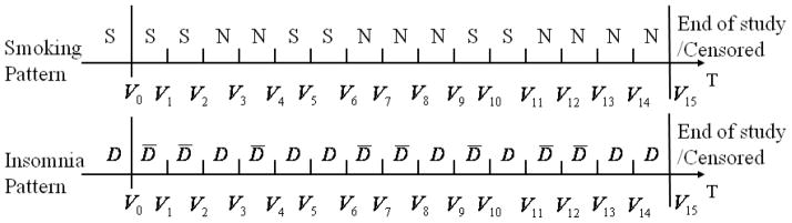
The smoking and insomnia patterns of one individual with S and N denoting smoking and nonsmoking, respectively, D and D̄ denoting insomnia and non-insomnia, respectively. The symbols before V₀ denote the baseline smoking and insomnia statuses.

Next, the correlation between two time-varying variables smoking and insomnia is explored. Let y_i1,t (1 if smoke, 0 otherwise) and y_i2,t (1 if insomnia, 0 otherwise) be the smoking and insomnia statuses of individual i (i = 1, …, m, m is the total number of individuals) at visit t (t = 0, …, v_i, where 0 is baseline visit and v_i is individual i’s total number of follow-up visits), respectively. Let y_i denote individual i’s outcome variable vector including both smoking and insomnia processes across all visits. The correlation at each time lag k is computed using logarithm of odds ratio (OR) defined as $OR(k)=n_{00}^{(k)}{n}_{11}^{(k)}/(n_{01}^{(k)}{n}_{10}^{(k)})$, where $n_{ab}^{(k)}={\sum }_{i=1}^m{n}_{\mathit{iab}}^{(k)}$ with a, b = 0 or 1, $n_{\mathit{iab}}^{(k)}$ is the total number of occurrences of y_i1,t−k = a and y_i2,t = b of individual i for t = 0, …, v_i + k if k < 0 and for t = k, …, v_i if k ≥ 0. For example, the individual displayed in Figure 1 has v_i = 15, $n_{i00}^{(-1)}=5,n_{i01}^{(-1)}=4,n_{i10}^{(-1)}=3,n_{i11}^{(-1)}=3$, for time lag −1, and $n_{i00}^{(1)}=4,n_{i01}^{(1)}=4,n_{i10}^{(1)}=4,n_{i11}^{(1)}=3$, for time lag 1.

Table 1 displays the log OR and the p values under different time lags k computed from 2, 849 individuals in the ATBC dataset who made at least one quit attempt and had at least one interval with insomnia symptom. It suggests that the correlation peaks at small lags, i.e., −1, 0, and 1, and decreases as the time lag increases. The negative sign in log OR at negative lags indicates that insomnia at the previous visits is associated with nonsmoking at the current visit, while the negative sign at positive lags indicates that smoking at the previous visits is associated with non-insomnia at the current visit. Smoking and insomnia are strongly correlated under small lags as indicated by the extremely small p-values, e.g., p = 1.50e − 18 at lag −1 and p = 1.83e − 18 at lag 1. Therefore, it is essential to consider the association between smoking and insomnia.

Table 1.

The log odds ratios and the p values under different time lag values.

lag	log OR	p
−4	−0.049	0.025
−3	−0.093	1.26e-05
−2	−0.138	2.91e-11
−1	−0.178	1.50e-18
0	−0.163	1.42e-16
1	−0.181	1.83e-18
2	−0.115	8.22e-08
3	−0.069	0.002
4	−0.052	0.003

2.2. The Joint Model

This section first illustrates a three-state discrete-time stochastic process with P_ij,t, j = 1, 2, 3, denoting individual i’s transition probabilities at visit t, as in Figure 2. This process distinguishes transient quitting state (temporarily non-smoking with subsequent relapse) from permanent quitting state (lifelong smoke-free, latent state due to censoring) because the processes describing them are different and the identification and quantification of the risk factors associated with permanent quitting are more relevant to smoking cessation and public health. Because all individuals in the ATBC study were smokers at baseline, let the stochastic process starts from the smoking state. When individual i is in the smoking state, he makes quit attempts at visit t with probability P_i1,t. Conditional on making a quit attempt at visit t, the individual may become a permanent quitter with probability P_i3,t+1 at visit t + 1. With probability 1 − P_i3,t+1, the individual enters the transient quitting state at visit t + 1, from which he has probability P_i2,t+1 to relapse back to the smoking state at visit t + 1. For example, the individual in Figure 1 makes a quit attempt at visit 2 (t = 2) with probability P_i1,2. With probability 1 − P_i3,3, he enters transient quitting state at visit 3, from which he sustains at visit 3 with probability 1 − P_i2,3, and relapses back to smoking at visit 4 with probability P_i2,4. Conditional on the transition probability P_ij,t, the transition to the next state is determined only by the current state and the previous state.

Figure 2.

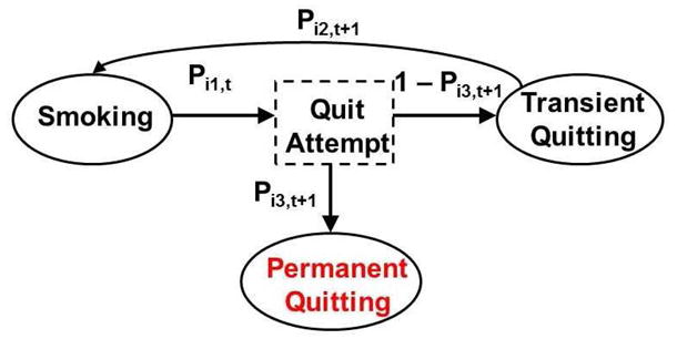
Transition among three states.

This modeling structure can be described using two types of geometric processes corresponding to the sojourn time distributions in the smoking and nonsmoking states. The first type (Type I) of geometric process describes the number of smoking intervals before the next quit attempt. After a quit attempt is made, the individual becomes permanent quitter with probability P_i3,t+1. The second type (Type II) of geometric process models the number of nonsmoking intervals before the next relapse, conditional on being in a transient quitting state. Figure 3 displays the partition of the stochastic smoking pattern and the longitudinal insomnia pattern of the individual in Figure 1. Visits 1 to 3 are modeled as a Type I geometric processes (denoted by I). The individual has an unsuccessful quit attempt (denoted by B) at visit 3 and enters the transient quitting state, which lasts until visit 5 (denoted by II). Conditional on having a relapse at visit 4, the individual transitions again into a Type I process at visit 5. The modeling continues using the same rules.

Figure 3.

The partitioned smoking and insomnia patterns with I and II denoting type I and II geometric processes, respectively, and B denoting unsuccessful quit attempt.

The likelihood of the smoking pattern for individual i (denoted by L_i1) is constructed by multiplying the likelihood contribution of both types of processes. For example, the likelihood of the smoking pattern for the individual in Figure 3 is

$$\begin{array}{l}{L}_{i1}=(1-P_{i1,0})(1-P_{i1,1})P_{i1,2}·(1-P_{i3,3})(1-P_{i2,3})P_{i2,4}·(1-P_{i1,5})P_{i1,6}\\ ·(1-P_{i3,7})(1-P_{i2,7})(1-P_{i2,8})P_{i2,9}·(1-P_{i1,10})P_{i1,11}\\ ·\{(1-P_{i3,12})(1-P_{i2,12})(1-P_{i2,13})(1-P_{i2,14})+P_{i3,12}\}.\end{array}$$

The term P_i3,12 at the end accounts for the probability of being a permanent quitter at visit 12.

Let P_i4,t be the probability of individual i having insomnia at visit t (referred to as the insomnia probability). Under conditional independence assumption (conditional on the random effect u_i4, P_i4,t1 and P_i4,t2 are independent for t₁ ≠ t₂), the likelihood of the insomnia pattern for individual i (denoted by L_i2) is obtained by multiplying the insomnia probabilities at all visits. For example, the likelihood of the insomnia pattern for the individual in Figure 3 is

$$\begin{array}{l}{L}_{i2}=(1-P_{i4,0})(1-P_{i4,1})P_{i4,2}·(1-P_{i4,3})P_{i4,4}·P_{i4,5}(1-P_{i4,6})\\ ·(1-P_{i4,7})P_{i4,8}(1-P_{i4,9})·P_{i4,10}(1-P_{i4,11})\\ ·(1-P_{i4,12})P_{i4,13}{P}_{i4,14}.\end{array}$$

For notational ease, the probability vector is denoted by ${\mathit{P}}_i={({\mathit{P}}_{i1}^{\prime },{\mathit{P}}_{i2}^{\prime },{\mathit{P}}_{i3}^{\prime },{\mathit{P}}_{i4}^{\prime })}^{\prime }$, where P_ij = (P_ij,1, …, P_ij,vi)′. The joint model for the smoking and insomnia processes has two sub-models.

$$\begin{array}{l}{g}_j(P_{ij,t}\mid {\mathit{x}}_{ij,t},y_{i2,t-1},u_{ij})={\mathit{x}}_{ij,t}{\mathit{\beta }}_{j0}+{\beta }_{j1}{y}_{i2,t-1}+u_{ij}\text{for}j=1,2,3;\\ g_4(P_{i4,t}\mid {\mathit{x}}_{i4,t},y_{i1,t-1},u_{i4})={\mathit{x}}_{i4,t}{\mathit{\beta }}_{40}+{\beta }_{41}{y}_{i1,t-1}+u_{i4},\end{array}$$ (1)

where the vectors x_ij,t and x_i4,t are covariate vectors which may include time-dependent covariates, and can share part of or all the covariates, y_i1,t−1 and y_i2,t−1 are the smoking and insomnia statuses at visit t − 1, respectively, u_ij and u_i4 are random effects, g(·) are link functions. Let g₁(·) and g₂(·) be the complementary log-log link function, g₃(·) and g₄(·) be the logit link function. The complementary log-log link function is used to make the transition probabilities between smoking and transient quitting states analogous to hazard functions in a discrete-time proportional hazards model [12].

To model the feedback effect, a single lagged covariate is included with the lag value being one [13]. Specifically, β_j1 denotes the feedback effect of the insomnia symptom at visit t − 1 (y_i2,t−1) on the smoking transition probability P_ij,t at visit t conditional on the covariate vector x_ij,t and the random effect u_ij. Similarly, β₄₁ represents the feedback effect of smoking at visit t − 1 (y_i1,t−1) on the insomnia probability at visit t conditional on the covariate vector x_i4,t and the random effect u_i4. For notational ease, the coefficient vector is denoted by $\mathit{\beta }={({\mathit{\beta }}_1^{\prime },{\mathit{\beta }}_2^{\prime },{\mathit{\beta }}_3^{\prime },{\mathit{\beta }}_4^{\prime })}^{\prime }$, where ${\mathit{\beta }}_j^{\prime }=({\mathit{\beta }}_{j0}^{\prime },{\beta }_{j1})$ for j = 1, 2, 3, and ${\mathit{\beta }}_4^{\prime }=({\mathit{\beta }}_{40}^{\prime },{\beta }_{41})$. For individual i, let x_i denote the covariate information, and let the multivariate random effect vector be u_i = (u_i1, u_i2, u_i3, u_i4)′.

The two sub-models in (1) are linked via the random effect vector u_i, which is assumed to be independent and identically distributed with normal probability density function u_i|Σ ~ N₄(0, Σ), where Σ is a 4 × 4 covariance matrix with the (l, m)th entry denoted by σ_lm. As pointed out by Molenberghs and Verbeke [14, Chap. 25.2], a special case of this model specification for random effects is the shared-parameter model, which assumes the same set of random effects for both smoking and insomnia outcomes in this context. While the shared-parameter model has relatively lower dimension of the random effects distribution when compared to the above model, it is based on much stronger assumptions about the association between outcomes, which is difficult to validate in this application.

The joint modeling framework has accounted for three sources of correlation, i.e., intra-process correlation (measurements from the same process at different visits), inter-process correlation (measurements from different processes at the same visit), and cross-process correlation (measurement from different processes at different visits). The intra-process correlation is modeled by the process-specific random effect u_i. The inter-process correlation is modeled by the association between u_i1, u_i2, u_i3 and u_i4 through three covariance parameters σ₄₁, σ₄₂, and σ₄₃. If the covariance parameters are significantly different from zero, it indicates the existence of the inter-process correlation. Finally, the cross-process correlation is modeled by the single lagged covariates y_i1,t−1 and y_i2,t−1, as well as three covariance parameters σ₄₁, σ₄₂, and σ₄₃.

It is assumed that the smoking process is independent of the insomnia process, conditional on the covariates and the random effect vector u_i. The observed likelihood conditional on u_i for individual i is L(Φ; u_i, y_i) = L_i1L_i2, where the parameter vector of interests Φ = {β, Σ}. The marginal likelihood is L(Φ; y_i) = ∫L(Φ; u_i, y_i)h(u_i; Σ)du_i, where h(u_i; Σ) is N₄(0, Σ). Because this integral cannot be evaluated analytically, the samples of the parameter vector Φ can be obtained using the Bayesian inference framework via Markov Chain Monte Carlo (MCMC) simulations introduced in Section 2.3.

2.3. Bayesian Inference

This section proposes a Bayesian approach for the model inference. Noninformative priors are used for the parameter vectors. Each component in the coefficient vector β is independently assigned normal N(0, 100) prior distribution. For the ease of sampling for Σ, an approach based on the Cholesky decomposition [15] is used. Let Σ = ΩΩ′, where Ω is a lower triangular matrix with ω_lm being the (l, m)th entry for 1 ≤ m ≤ l ≤ 4 and zero entries above the main diagonal. Consider a latent vector z_i = (z_i1, …, z_i4)′ with N(0, 1) independent components. The linear reparameterization of u_i = Ωz_i (with element being $u_{ij}={\sum }_{l=1}^j{\omega }_{jl}{z}_{il}$, e.g., u_i2 = ω₂₁z_i1 + ω₂₂z_i2) has mean zero and variance Σ, whose entries are ${\sigma }_{jk}={\sum }_{l=1}^{j\wedge k}{\omega }_{jl}{\omega }_{kl}$, 1 ≤ j, k ≤ 4, where j ∧ k = min(j, k). Uniform(0, 10) prior distribution is imposed on ω_ll to ensure non-negativity and N(0, 100) prior distribution on ω_lm when l ≠ m to allow for possible negative correlation. For notational ease, let vectors σ and ω denote the entries in the lower triangular part of the matrices Σ and Ω, respectively, and let vector ρ = (ρ₂₁, ρ₃₁, ρ₃₂, ρ₄₁, ρ₄₂, ρ₄₃) denote the pairwise correlation coefficients among the components of the random effects vector u_i.

The joint distribution of the data and parameters is

$$P(\mathit{\beta },\mathit{\sum })=\prod _{i=1}^m\left[L_{i1}{L}_{i2}\left\{\prod _{j=1}^{4}p({\mathit{P}}_{ij};{\mathit{\beta }}_j,\mathit{\omega },{\mathit{z}}_i)P({\mathit{z}}_i)\right\}\right]P(\mathit{\beta })P(\mathit{\omega }),$$ (2)

where P(β), and P(ω) are the prior distributions of β and ω, respectively. The full conditional distributions are derived and the parameters are sampled component-wise using a random walk Metropolis-Hastings algorithm in the following order (β₁, ω₁₁), (β₂, ω₂₁, ω₂₂), (β₃, ω₃₁, ω₃₂, ω₃₃), (β₄, ω₄₁, ω₄₂, ω₄₃, ω₄₄), and z_i. The posterior distributions of σ and ρ are computed from the posterior samples of ω. For statistical inference, the posterior means, standard deviations, and 95% equal-tail credible intervals (i.e., the intervals from 2.5 and 97.5 percentiles of the posterior distributions) are computed.

To assess the convergence of the MCMC chains, the trace plots are used and the absence of apparent trend in the plots is viewed as evidence of convergence. In addition, multiple chains with overdispersed initial values are run and the Gelman-Rubin scale reduction statistics R̂ are computed to ensure R̂ of all parameters are smaller than 1.1 [16]. The length of the burn-in is assessed by trace plots and autocorrelation for each parameter.

3. Simulation Studies

In this section, two simulation studies are conducted to compare the performance of the proposed joint model and a separate model, i.e., separately fitting a three-state stochastic process model for the smoking pattern and a generalized linear mixed model (GLMM) for the longitudinal insomnia process. In the first simulation study, there is no inter-process correlation (i.e., σ₄₁, σ₄₂, σ₄₃ = 0), while in the second simulation study, there exists large inter-process correlation. In both simulation studies, 500 datasets with sample size m = 10, 000 and with data structure similar to the ATBC dataset are generated. We consider the case where the smoking transition probabilities only depend on the insomnia status at the last visit and the insomnia probability only depends on the smoking status at the last visit. No missing data are generated. The smoking and insomnia processes are generated using the following algorithm.

1. For individual i, simulate the total visit number from a normal distribution with mean 14.2 and standard deviation 6.3, because it resembles the distribution of the number of follow-up visits in the ATBC study. Round the total visit number to the closest integer if it is larger than 1 and round it to 1 if it is smaller than 1.

2. Simulate the random effects vector u_i from multivariate normal distribution with mean 0 and covariance matrix

   $$\mathit{\sum }=\left(\begin{array}{cccc}\hfill 0.09& \hfill -0.01& \hfill -0.12& 0\\ \hfill -0.01& \hfill 0.16& \hfill 0.05& 0\\ \hfill -0.12& \hfill 0.05& \hfill 0.25& 0\\ 0& 0& 0& 0.36\end{array}\right).$$

   for the first simulation study. The correlation coefficients among the components of u_i are (ρ₂₁, ρ₃₁, ρ₃₂, ρ₄₁, ρ₄₂, ρ₄₃) = (−0.083, −0.8, 0.25, 0, 0, 0). In the second simulation study, let (σ₄₁, σ₄₂, σ₄₃) = (−0.05, −0.04, 0.05), which gives inter-process correlation coefficients (ρ₄₁, ρ₄₂, ρ₄₃) = (−0.28, −0.17, 0.17).

3. Simulate the baseline insomnia status from a Bernoulli distribution with the success probability 0.2, because the prevalence of baseline insomnia symptom is around 20%. The probability P_ij for j = 1, 2, 3 and P_i4 at the first visit are computed from model (1) with β₁ = (0.186, −1.217)′, β₂ = (−1.031, 1.217)′, β₃ = (0.405, −2.603)′, and β₄ = (−2, 1)′. Let y_i1,0 = 1 because every individual is a smoker at baseline in the ATBC study.

4. Conditional on smoking at visit t − 1, simulate the insomnia status at visit t from a Bernoulli distribution with probability P_i4,t and simulate the smoking status at visit t from a Bernoulli distribution with probability P_i1,t.

5. Conditional on making a quit attempt at visit t, simulate the quitting status as follows.

   1. With probability P_i3,t+1, the individual becomes a permanent quitter, and all the remaining visits are nonsmoking. Simulate the insomnia status at the remaining visits with probability P_i4,t+1.

   2. With probability 1 − P_i3,t+1, the individual becomes a transient quitter. The smoking and insomnia statuses at visit t + 1 are simulated with probability P_i2,t+1 and P_i4,t+1, respectively.

6. Compute P_ij,t+1 for j = 1, 2, 3 and P_i4,t+1 at visit t + 1 conditional on the smoking and insomnia statuses at visit t.

7. Repeat Steps 4, 5, and 6 until a smoking pattern and an insomnia pattern are generated for each individual.

The Bayesian framework in Section 2.3 is applied to obtain samples from the posterior distributions of the parameters of interest. For each dataset in both simulation studies, three parallel chains with overdispersed initial values are run. Each chain is run for 50, 000 iterations, the first 20, 000 iterations are discarded as a burn-in, and the next 30, 000 samples are used to calculate the joint posterior distribution of the parameters of interest.

The results of the separate model and the joint model of the first simulation study with no inter-process correlation are compared in Table 2. In this table, we label the average of the posterior means minus the true values as bias, the square root of the average of the variances as SE, the standard deviation of the posterior means as SD, the coverage probabilities of 95% equal-tail credible intervals (CI) as CP, and the square root of the average of the squares of the bias as root mean square error (RMSE). The results suggest that two methods generate comparable results, i.e., the bias is negligible, SE is close to SD, the credible interval coverage probabilities are reasonably close to 95%, and RMSE is comparable. The estimates of σ₄₁, σ₄₂, and σ₄₃ from the joint model are correctly close to zero although the standard errors of σ₄₂ and σ₄₃ are slightly underestimated, which leads to conservative credible intervals and the coverage probability being smaller than the nominal value.

Table 2.

Bias, standard error (SE), standard deviation (SD), and coverage probabilities (CP) of 95% credible intervals, for the separate model and the joint model, when there is no inter-process correlation.

Parameter	Separate Model					Joint Model
	Bias	SE	SD	CP	RMSE	Bias	SE	SD	CP	RMSE
β10 = 0.186	−0.001	0.010	0.010	0.958	0.011	−0.003	0.010	0.011	0.940	0.011
β11 = −1.217	0.000	0.024	0.023	0.970	0.023	0.001	0.024	0.023	0.968	0.023
β20 = −1.031	0.001	0.026	0.025	0.946	0.025	−0.002	0.027	0.028	0.928	0.028
β21 = 1.217	−0.002	0.024	0.026	0.920	0.026	−0.002	0.026	0.026	0.944	0.026
β30 = 0.405	0.006	0.026	0.025	0.976	0.025	−0.001	0.025	0.024	0.970	0.024
β31 = −2.603	−0.013	0.063	0.069	0.922	0.070	0.006	0.068	0.070	0.914	0.070
β40 = −2.000	−0.001	0.012	0.013	0.930	0.013	−0.001	0.012	0.013	0.922	0.013
β41 = 1.000	0.000	0.016	0.015	0.960	0.015	0.000	0.017	0.016	0.938	0.016
σ11 = 0.090	0.000	0.010	0.009	0.940	0.009	−0.002	0.009	0.010	0.916	0.011
σ21 = −0.010	0.000	0.011	0.012	0.906	0.012	0.000	0.011	0.013	0.910	0.013
σ22 = 0.160	0.003	0.023	0.022	0.944	0.023	−0.002	0.024	0.026	0.924	0.026
σ31 = −0.120	0.001	0.015	0.016	0.924	0.016	−0.004	0.016	0.017	0.924	0.018
σ32 = 0.050	0.002	0.033	0.031	0.948	0.031	−0.006	0.034	0.036	0.922	0.036
σ33 = 0.250	0.024	0.063	0.067	0.944	0.071	−0.014	0.062	0.063	0.928	0.065
σ44 = 0.360	0.002	0.014	0.013	0.960	0.013	0.002	0.014	0.013	0.950	0.013
σ41 = 0.000						−0.001	0.008	0.008	0.914	0.008
σ42 = 0.000						−0.001	0.013	0.015	0.880	0.015
σ43 = 0.000						0.001	0.016	0.019	0.880	0.019

Table 3 displays the results of the second simulation study with large inter-process correlation. The results from the joint model indicate that the estimates of all parameters, including the inter-process correlation coefficients, have negligible bias, SE being close to SD. The coverage probabilities of 95% credible intervals are all reasonably around the nominal value. In contrast, the separate model gives biased estimates, low coverage probabilities, and larger RMSE for the insomnia effect in modeling the smoking transition probabilities (β₁₁, β₂₁, and β₃₁, shown in boldface), due to ignoring the inter-process correlation, and the consequent information loss. There is no apparent difference in the estimation of the longitudinal insomnia process comparing the separate model to the joint model.

Table 3.

Bias, standard error (SE), standard deviation (SD), and coverage probabilities (CP) of 95% credible intervals, for the separate model and the joint model, when there is sizeable inter-process correlation.

Parameter	Separate Model					Joint Model
	Bias	SE	SD	CP	RMSE	Bias	SE	SD	CP	RMSE
β10 = 0.186	−0.002	0.010	0.009	0.948	0.010	−0.001	0.010	0.010	0.958	0.010
β11 = −1.217	−0.030	0.024	0.025	0.766	0.039	−0.006	0.025	0.026	0.926	0.027
β20 = −1.031	−0.002	0.026	0.024	0.950	0.024	−0.006	0.031	0.033	0.922	0.034
β21 = 1.217	−0.028	0.024	0.022	0.848	0.036	−0.004	0.026	0.027	0.926	0.027
β30 = 0.405	−0.007	0.026	0.026	0.948	0.027	−0.004	0.025	0.026	0.934	0.027
β31 = −2.603	0.032	0.063	0.063	0.886	0.070	0.002	0.064	0.066	0.938	0.066
β40 = −2.000	−0.001	0.011	0.012	0.930	0.012	0.000	0.012	0.012	0.922	0.012
β41 = 1.000	0.006	0.016	0.016	0.910	0.017	0.000	0.017	0.017	0.952	0.017
σ11 = 0.090	−0.002	0.009	0.010	0.924	0.010	−0.003	0.010	0.011	0.922	0.011
σ21 = −0.010	−0.003	0.011	0.011	0.908	0.012	0.002	0.020	0.022	0.932	0.023
σ22 = 0.160	0.005	0.023	0.024	0.950	0.024	−0.009	0.040	0.044	0.942	0.044
σ31 = −0.120	0.002	0.015	0.016	0.904	0.016	0.003	0.017	0.019	0.924	0.019
σ32 = 0.050	−0.003	0.032	0.035	0.920	0.035	−0.007	0.044	0.045	0.924	0.046
σ33 = 0.250	0.010	0.060	0.059	0.960	0.059	−0.013	0.061	0.063	0.944	0.064
σ44 = 0.360	0.001	0.014	0.015	0.910	0.015	0.002	0.014	0.015	0.916	0.015
σ41 = −0.050						0.001	0.008	0.010	0.930	0.010
σ42 = −0.040						0.006	0.016	0.019	0.918	0.020
σ43 = 0.050						0.003	0.017	0.019	0.944	0.019

Note: Large bias and poor CP are highlighted in boldface.

From the simulation studies, the conclusion is that the joint model provides results comparable to the separate model when there is no inter-process correlation, while it provides more accurate estimates for the smoking process than the separate model when the inter-process correlation is large.

4. Application to the ATBC Study

In this section, the proposed joint model and the Bayesian inference framework are applied to the motivating ATBC dataset. For all the results in this section, three parallel chains with overdispersed initial values are used, and each chain is run for 150, 000 iterations. The first 50, 000 iterations are discarded as burn-in and the inference is based on the remaining 100, 000 iterations. The results from the separate model and from the joint model are compared.

We fit models with the following covariates: smoking or insomnia status at the last visit, and baseline covariates including age, years of smoking, cigarettes per day, alcohol consumption (g/day), and inhalation (yes/no). Table 4 shows the estimation results with a negative sign indicating a smaller probability of having a certain event. It is observed that the joint model and the separate model give different estimates (highlighted in boldface) for the insomnia effect in modeling the smoking transition probabilities, although the same set of parameters are identified for significance by both models. For example, conditional on the random effect u_i1, both models indicate that individuals with insomnia at the last visit have higher probability to make quit attempts than those without insomnia. In addition, conditional on u_i2, and u_i3, the joint model results suggest that insomnia at the last visit is associated with higher probability of relapse and permanent quitting given the quit attempts, while the separate model results suggest the association in opposite direction. The differences between the results from the joint model and the separate model might be explained by the significant high negative inter-process correlation coefficients (ρ̂₄₁ = −0.051, ρ̂₄₂ = −0.274, and ρ̂₄₃ = −0.141). With the help of jointly modeling the correlated stochastic smoking process and the longitudinal insomnia process, the joint model is expected to improve the estimation of the parameters of insomnia effects, as demonstrated in Section 3.

Table 4.

Results of fitting the separate model and the joint model with six covariates in the ATBC dataset. Entries in boldface indicate different results from the two models.

Models	Parameters	Separate Model			Joint Model
		MeanSD	95% CI		MeanSD	95% CI
Pi1	Intercept	−4.4090.026	−4.463	−4.359	−4.4250.027	−4.479	−4.372
	Insomnia*	0.2100.036	0.138	0.281	0.2810.043	0.198	0.362
	Age*	0.1950.017	0.162	0.228	0.1950.016	0.163	0.228
	Years smoked*	−0.2710.015	−0.301	−0.242	−0.2740.015	−0.303	−0.246
	Cigarette/day*	−0.2950.016	−0.326	−0.264	−0.2950.016	−0.329	−0.266
	Alcohol*	−0.1990.018	−0.234	−0.162	−0.2020.018	−0.238	−0.165
	Inhale	0.0060.029	−0.050	0.062	0.0080.030	−0.047	0.067
Pi2	Intercept	−0.5500.214	−0.958	−0.121	−0.4400.235	−0.866	0.018
	Insomnia	−0.0140.091	−0.192	0.163	0.1230.094	−0.061	0.305
	Age	0.0080.058	−0.102	0.124	−0.0070.058	−0.120	0.105
	Years smoked	−0.0300.050	−0.128	0.069	−0.0140.051	−0.108	0.087
	Cigarette/day*	−0.1440.054	−0.250	−0.040	−0.1400.051	−0.239	−0.035
	Alcohol	0.1320.068	−0.006	0.265	0.1000.067	−0.032	0.240
	Inhale	0.0500.097	−0.141	0.241	0.0250.095	−0.165	0.211
Pi3	Intercept	2.6110.214	2.214	3.048	2.7190.244	2.284	3.224
	Insomnia	−0.2620.146	−0.549	0.022	0.0610.189	−0.317	0.431
	Age	0.0710.066	−0.059	0.200	0.0530.071	−0.085	0.193
	Years smoked*	0.1320.058	0.022	0.248	0.1500.062	0.026	0.275
	Cigarette/day	0.0330.065	−0.095	0.159	0.0330.063	−0.091	0.160
	Alcohol	0.0030.073	−0.141	0.147	−0.0260.077	−0.176	0.133
	Inhale	−0.0240.115	−0.251	0.204	−0.0540.124	−0.300	0.185
Pi4	Intercept	−3.7980.040	−3.871	−3.713	−3.7720.044	−3.856	−3.685
	Smoking*	−0.3530.028	−0.410	−0.300	−0.3900.032	−0.455	−0.335
	Age*	0.1910.027	0.131	0.252	0.1790.031	0.123	0.251
	Years smoked	0.0190.030	−0.042	0.076	0.0350.034	−0.034	0.113
	Cigarette/day*	0.1250.024	0.087	0.180	0.1190.025	0.073	0.176
	Alcohol*	0.3440.021	0.304	0.393	0.3600.028	0.306	0.408
	Inhale*	0.1250.058	0.009	0.253	0.1320.048	0.039	0.225
ρ	ρ21	−0.1250.112	−0.340	0.109	−0.1480.124	−0.380	0.111
	ρ31	−0.9620.022	−0.994	−0.909	−0.9200.026	−0.963	−0.863
	ρ32	0.3540.141	0.067	0.607	0.4590.135	0.181	0.690
	ρ41				−0.0510.019	−0.081	−0.015
	ρ42				−0.2740.028	−0.339	−0.231
	ρ43				−0.1410.032	−0.205	−0.077

Note:

^*represents statistical significance.

The joint model and the separate model produce similar results for other parameters in terms of means, standard deviations, and 95% CIs and identified similar set of significant covariates. The rows labeled P_i1 in Table 4 display the results of modeling the probability of making quit attempts at a given visit. We conclude that conditional on the random effect u_i1, individuals with insomnia at the last visit or older individuals are more likely to make quit attempts, while years of smoking, cigarettes per day, and alcohol consumption are negatively associated with the probability of making quit attempts. The rows labeled P_i2 in Table 4 display the results of modeling the probability of relapsing at a given visit for individuals in the transient quitting stage. It suggests that conditional on the random effect u_i2, individuals who smoke more cigarettes per day are less likely to relapse once they make quit attempts. This unexpected results have been identified and reported in the previous works [10, 11]. The rows labeled P_i3 in Table 4 display the results of modeling the probability of permanent quitting at a certain visit. Conditional on the random effect u_i3, individuals with longer smoking history are more likely to be permanent quitter once quit attempt are made, i.e., the odds ratio of permanent quitting for an increase of 8.4 years of smoking history (i.e., one standard deviation) is 1.162 (95% CI: [1.026, 1.317]), holding other covariates fixed. The rows labeled P_i4 in Table 4 display the results of modeling the probability of insomnia at a certain visit. Conditional on the random effect u_i4, smoking at the last visit is negatively associated with the insomnia probability, while age, years of smoking, cigarettes per day, alcohol consumption, and inhalation show positive association.

The data analysis results suggests the existence of a feedback system. First, conditional on the random effect u_i1, the complement probability of making quit attempts for individuals with insomnia at the last visit is the complement probability for those without insomnia raised to the power 1.324 (95% CI: [1.219, 1.436]). Moreover, conditional on the random effect u_i4, the odds ratio of having insomnia for individuals who did not smoke at the last visit is 1.477 (95% CI: [1.398, 1.576]), compared with those who smoked. Hence insomnia increases the likelihood of making quit attempts which further increases the risk of future insomnia in a feedback cycle. These results of the feedback system are consistent with the negative smoking and insomnia correlations displayed in Table 1.

Our model identifies a high negative correlation between P_i1 and P_i3 (ρ₃₁), and a relative high positive correlation between P_i2 and P_i3 (ρ₃₂). We now provide some insight about these high correlations. Consider ρ̂₃₁ first. There are 1, 501 long-term sustainers (individuals who sustained at least 40 months until censoring) who are more likely to be permanent quitters and hence have high P_i3. Among them, 1, 453 (96.8%) made only one quit attempt. The association of high P_i3 (long trailing non-smoking intervals) with small P_i1 (only one quit attempt) leads to high negative ρ₃₁. Consider ρ̂₃₂ next. The 1, 115 relapsers (individuals who made at least one quit attempt but did not sustain until censoring) had an average smoke-free interval of 2.56 visits (10.2 months) before next relapse. The association of small P_i3 (relapse frequently with not trailing nonsmoking interval) and small P_i2 (long smoke-free interval) leads to high positive ρ₃₂.

Table 4 displays strong correlation between the stochastic smoking process and the longitudinal insomnia process, e.g., high negative correlation between P_i1 and P_i4 (ρ₄₁), between P_i2 and P_i4 (ρ₄₂), and between P_i3 and P_i4 (ρ₄₃). Here, some insight into this interesting phenomenon is provided. Let us first consider ρ̂₄₁. There are 6, 034 ever-quitters (individuals who made at least one quit attempt) and 20, 181 never-quitters (individuals who never made any quit attempts). In our model, the ever-quitters are more likely to have larger probabilities of making quit attempts. The empirical estimate of probability of insomnia is smaller among ever-quitters than among never-quitters (i.e., mean: 0.131 v.s. 0.144, p < 0.001). The association of larger probabilities of making quit attempts and smaller probabilities of insomnia indicates negative correlation of ρ₄₁. Next, ρ̂₄₂ is considered. There are 15, 757 non-insomnia individuals (individuals who never had insomnia) and 10, 458 insomnia individuals (individuals who had insomnia at least one visit). In our model, non-insomnia individuals are more likely to have smaller probabilities of insomnia than the insomnia individuals. Among them, there are 3, 495 and 2, 539 individuals who made at least one quit attempt, respectively. The non-insomnia individuals have shorter smoke-free intervals before relapse than the insomnia individuals (i.e., 0.6 months v.s. 2.2 months, p < 0.001). The association of smaller probabilities of insomnia and higher relapse probabilities P_i2 (shorter smoke-free intervals) indicates negative correlation of ρ₄₂. At last, ρ̂₄₃ is considered. There are 1, 501 long-term sustainers and 1, 115 relapsers. In our model, the long-term sustainers are more likely to have higher permanent quitting probabilities than the relapsers. The empirical estimate of probability of insomnia is smaller among long-term sustainers than relapsers (i.e., mean: 0.124 v.s. 0.140, p = 0.10). The association of higher permanent quitting probabilities with smaller probabilities of insomnia indicates negative correlation.

5. Discussion

In this article, we propose a joint model and a Bayesian approach to analyze the longitudinal insomnia process and the stochastic smoking process with a latent cure state. By combining the information from the longitudinal data, the joint model improves the accuracy of the parameter estimates compared with the separate model and provides similar precision, when strong inter-process correlation exists. On the other hand, the joint model produces comparable results to the separate model when there is no inter-process correlation. Our joint model extends the functionality of the modeling framework in Luo et al [11] by including time-dependent covariates and by accounting for the correlation between the subject-specific smoking transition probabilities and the insomnia probability. Consequently, significant negative correlation between the smoking and insomnia processes is identified. An important but previously unknown finding is the existence of a feedback system between insomnia and smoking, e.g., insomnia at the last visit increases the likelihood of making quit attempts at the current visit which further increases the risk of future insomnia in a feedback cycle. In addition, insomnia at the last visit has shown significant positive association with the probability of making quit attempts but insignificant positive association with the probabilities of relapse and permanent quitting given the quit attempts.

The proposed joint modeling framework is attractive in several respects. First, the joint model provides correction of potential biases in the separate model when the insomnia and smoking processes are strongly correlated. Second, the joint model accounts for and provides insight into the within-subject correlation between the insomnia and smoking processes. Third, we develop a method to formulate and calculate the likelihood function involving time-dependent covariates. To the best of our knowledge, this article is the first one to propose a joint model for a stochastic process and a longitudinal outcome with time-dependent covariates. Computationally, the proposed Bayesian inference method can account for high-dimensional random effects and it also allows incorporation of prior information.

The proposed joint model is flexible enough to address many questions of scientific interest. For example, if it is of interest to jointly model more longitudinal measurements of diseases with the smoking process, P_i4,t in model (1) could be expanded to a vector of probabilities with each component representing the probability of the presence of each disease. Additionally, more time-dependent covariates (e.g., the participation of a smoking cessation program or the increase of cigarette tax) can be incorporated into the model to estimate the effects of these covariates.

The smoking and insomnia information in the ATBC dataset is based on 4-month interval and visit-to-visit transitions of smoking status are modeled while some recent articles on the analysis of smoking cessation data modeled the smoking transition in a more continuous manner [17, 18]. One limitation of the proposed model is that the cross-process correlation is modeled by the single lagged covariates and the covariance parameters σ₄₁, σ₄₂, and σ₄₃. It is difficult to distinguish the contribution of each source. We will address this issue in our future research. Another issue is the normality assumption of random effects in our joint model. Some researchers [19, 20] have reported that the statistical inference is generally robust to the departure from the normality assumption. It is of interest to investigate our joint model’s performance when the underlying random effects distribution is symmetric non-normal or even asymmetric. Moreover, the random effects covariance matrix is assumed to be homogeneous (same for all individuals). However, the covariance matrix may depend on subject-specific characteristics and is thus heterogeneous. Ignoring the heterogeneity can result in biased estimates [21, 22]. As a future direction, we would address the issue of accounting for heterogeneity in the covariance matrix in the proposed joint modeling framework.

References

- 1.Bixler EO, Kales A, Soldatos CR, Kales JD, Healey S. Prevalence of sleep disorders in the Los Angeles metropolitan area. The American Journal of Psychiatry. 1979;136:1257–1262. doi: 10.1176/ajp.136.10.1257. [DOI] [PubMed] [Google Scholar]
- 2.Mellinger GD, Balter MB, Uhlenhuth EH. Insomnia and its treatment. prevalence and correlates. Archives of General Psychiatry. 1985;42:225–232. doi: 10.1001/archpsyc.1985.01790260019002. [DOI] [PubMed] [Google Scholar]
- 3.Ford DE, Kamerow DB. Epidemiologic study of sleep disturbances and psychiatric disorders. an opportunity for prevention? The Journal of American Medical Association. 1989;262:1479–1484. doi: 10.1001/jama.262.11.1479. [DOI] [PubMed] [Google Scholar]
- 4.Prochaska JO, DiClemente CC. Stages and processes of self-change of smoking: toward an integrative model of change. Journal of Consulting and Clinical Psychology. 1983;31:390–395. doi: 10.1037//0022-006x.51.3.390. [DOI] [PubMed] [Google Scholar]
- 5.Wetter DW, Young TB. The relation between cigarette smoking and sleep disturbance. Preventive Medicine. 1994;23:328–334. doi: 10.1006/pmed.1994.1046. [DOI] [PubMed] [Google Scholar]
- 6.Phillips B, Mannino DM. Do insomnia complaints cause hypertension or cardiovascular disease? Journal of Clinical Sleep Medicine. 2007;3:489–94. [PMC free article] [PubMed] [Google Scholar]
- 7.Hughes JR. Effects of abstinence from tobacco: valid symptoms and time course. Nicotine & Tobacco Research. 2007;9:315–327. doi: 10.1080/14622200701188919. [DOI] [PubMed] [Google Scholar]
- 8.Zeger SL, Liang KY. Feedback models for discrete and continuous time series. Statistica Sinica. 1991;1:51–64. [Google Scholar]
- 9.Group AS. Incidence of cancer and mortality following α-tocopherol and β-carotene supplementation. Journal of American Medical Association. 2003;290(4):476–485. doi: 10.1001/jama.290.4.476. [DOI] [PubMed] [Google Scholar]
- 10.Luo S, Crainiceanu CM, Louis TA, Chatterjee N. Analysis of smoking cessation patterns using a stochastic mixed-effects model with a latent cured state. Journal of the American Statistical Association. 2008;103:1002–13. doi: 10.1198/016214507000001030. [DOI] [PMC free article] [PubMed] [Google Scholar]
- 11.Luo S, Crainiceanu CM, Louis TA, Chatterjee N. Bayesian inference for smoking cessation with a latent cure state. Biometrics. 2009;65:970–978. doi: 10.1111/j.1541-0420.2008.01167.x. [DOI] [PMC free article] [PubMed] [Google Scholar]
- 12.Kalbfleisch J, Prentice RL. The Statistical Analysis of Failure Time Data. John Wiley & Sons; 2002. [Google Scholar]
- 13.Diggle PJ, Heagerty P, Liang KY, Zeger SL. Analysis of Longitudinal Data. Oxford University Press; 2002. [Google Scholar]
- 14.Molenberghs G, Verbeke G. Models for Discrete Longitudinal Data. Springer Verlag; 2005. [Google Scholar]
- 15.Anderson T. An Introduction to Multivariate Statistical Analysis. 3. John Wiley & Sons; 2003. [Google Scholar]
- 16.Gelman A, Carlin J, Stern H, Rubin D. Bayesian Data Dnalysis. CRC press; 2004. [Google Scholar]
- 17.Li Y, Wileyto EP, Heitjan DF. Modeling smoking cessation data with alternating states and a cure fraction using frailty models. Statistics in Medicine. 2010;29(6):627–638. doi: 10.1002/sim.3825. [DOI] [PMC free article] [PubMed] [Google Scholar]
- 18.Li Y, Wileyto EP, Heitjan DF. Prediction of individual long-term outcomes in smoking cessation trials using frailty models. Biometrics. 2011;67:1321–1329. doi: 10.1111/j.1541-0420.2011.01578.x. [DOI] [PubMed] [Google Scholar]
- 19.Song X, Davidian M, Tsiatis AA. A semiparametric likelihood approach to joint modeling of longitudinal and time-to-event data. Biometrics. 2002;58(4):742–753. doi: 10.1111/j.0006-341x.2002.00742.x. [DOI] [PubMed] [Google Scholar]
- 20.Zeng D, Cai J. Asymptotic results for maximum likelihood estimators in joint analysis of repeated measurements and survival time. The Annals of Statistics. 2005;33(5):2132–2163. [Google Scholar]
- 21.Heagerty PJ, Kurland BF. Misspecified maximum likelihood estimates and generalised linear mixed models. Biometrika. 2001;88(4):973. [Google Scholar]
- 22.Daniels MJ, Zhao YD. Modelling the random effects covariance matrix in longitudinal data. Statistics in Medicine. 2003;22(10):1631–1647. doi: 10.1002/sim.1470. [DOI] [PMC free article] [PubMed] [Google Scholar]