

Abstract
How do populations of neurons work together to control behavior? To study this issue, our group simultaneously records from populations of neurons across multiple electrodes in multiple brain regions during operant behavior. In this chapter, we describe methods for quantifying the relationship between neuronal population activity and performance of operant behavioral tasks. We describe statistical techniques, based on time- and trial-shuffling, that can establish the significance of correlations between multiple and simultaneously recorded spike trains. Then, we describe several approaches to studying functional interactions between neurons, including principal component analysis, cross-correlation analysis, analyses of rate correlations, and analyses of shared predictive information. Finally, we compare these techniques using a sample dataset and discuss how the combined used of these techniques can lead to novel insights regarding neuronal interactions during behavior.
Keywords: neural coding, neural ensemble, population activity, correlated variability, JPSTH, multi-electrode recordings
INTRODUCTION
Recent developments in electrode recording technology have facilitated recordings of neuronal population activity (Nicolelis, 1998; Nicolelis et al., 1998). Such techniques can generate data from hundreds of simultaneously recorded neurons in multiple brain areas (Carmena et al., 2003; Wessberg et al., 2000). To analyze such data, a multivariate approach is applied to firing rates of simultaneously collected neurons (Laubach et al., 2007). This approach can generate stable predictions from neuronal ensemble data about a behavioral variable (Laubach et al., 2000) or can be used as control signals for prosthetic devices (Wessberg et al., 2000).
Analyses of neuronal population data do not automatically offer insight about how neurons interact during behavior. This is in part due to the complications induced by neuroanatomy. In the cerebral cortex, neurons form thousands of synapses with other cortical neurons in neighboring and distant brain areas and have descending and recurrent connections to subcortical systems (Shepherd, 2003). Moreover, cortical neurons are typically embedded in a processing unit such as a column or local microcircuit (Mountcastle, 1998). As such, cortical neurons can have distinct non-synaptic functional relationships with neurons within and outside of their local processing units.
There have been mixed opinions in the literature about whether functional interactions between neurons underlie the encoding of behaviorally relevant information. Some studies have argued that interactions have little impact on information processing by neurons (Britten et al., 1996; Gochin et al., 1994; Reich et al., 2001; Rolls et al., 2004; Rolls et al., 1997). Other studies have presented strong evidence that that interactions between neurons may be an central feature of neural coding (Averbeck et al., 2003; Averbeck and Lee, 2003; Averbeck and Lee, 2004; Dan et al., 1998; Narayanan et al., 2005; Vaadia et al., 1995; Wessberg et al., 2000; Zohary et al., 1994). To establish the relevance of functional interactions to understanding how populations of neurons control behavior, neuronal population data must be studied with a variety of techniques and must be studied in awake, behaving animals using behavioral tasks that challenge the brain areas of interest (see Narayanan et al., 2006 and Narayanan and Laubach 2006 for an example of this approach).
In this chapter, we describe seven distinct techniques for investigating functional interactions between neurons: functional grouping by principal component analysis, cross-correlation, joint-peristimulus time histograms, rate correlations, trial-by-trial rate correlations, predictive interactions, and network interactions. We also establish significance of interaction based on time-shuffling or trial-shuffling spike trains. We then apply each of these techniques to a population of simultaneously recorded neurons from the rodent dorsomedial prefrontal cortex (dmPFC) and motor cortex. We use each of these techniques to generate insights into how neurons interact; and then we combine these techniques to derive a portrait of neuronal interactions across each cortical area.
METHODS
Neurophysiological Recordings
The multi-electrode data used in this chapter were collected from the rodent dorsomedial prefrontal cortex (dmPFC; comprising prelimbic and anterior cingulate cortex) and motor cortex of one rat during performance of a delayed-response task with a fixed 1.0 s delay (Narayanan et al., 2006). In this task, animals had to initiate and maintain a lever press for 1.0 s, and then release the lever promptly to get a liquid reward (Fig 1A). Twenty-one neurons (11 in motor cortex, 10 in dmPFC) were isolated from one animal during delayed-response performance. Methods used to acquire such data as well as the response properties of single neurons in these areas are described elsewhere in detail (Narayanan et al., 2006; Narayanan et al., 2005; Narayanan and Laubach, 2006). Briefly, electrical signals from each electrode in dmPFC and motor cortex are amplified, analog filtered, and streamed to a computer using a Multi-channel Acquisition Processor (MAP; Plexon, Dallas, TX). Putative single neuronal units were identified on-line using an oscilloscope and audio monitor. Cable noise and behavioral artifact is then cleaned using principal component projections of potential single units in Plexon’s Offline Sorter. Peri-stimulus arrays of activity around behavioral events of interest are then constructed and explorer using NeuroExplorer (Nex Technologies; Littleton, MA). All further analyses are performed using custom-written scripts for MATLAB (The Mathworks, Natick, MA) (Fig 1B).
Figure 1.
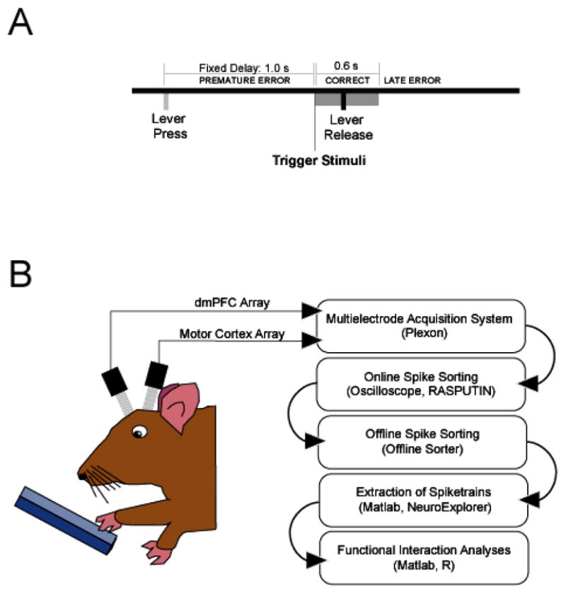
Methods for multi-electrode recordings in freely behaving animals. A) Sequence of events in delayed-response tasks. Rats were trained in a fixed-delay task, in which they had to initiate trials by pressing a lever until the end of a fixed (1.0 s) delay period. Rats had to release the lever within a designated response window to collect a liquid reward (Correct responses). If the lever was released before the trigger stimulus (Premature error responses) or after the response window (Late error responses), rats experienced a timeout period. After rats performed the fixed delay task, animals were re-trained on a delayed-response with two delays for three days. B) Methods for collection of multi-electrode data. Briefly, neurophysiological data are collected from the awake, behaving rats implanted with arrays of electrodes (2 16 wire microwire electrode arrays in dmPFC and motor cortex) during performance of a delayed response task. Data are streamed to a computer, sorted on-line using an oscilloscope, cleaned offline using principal component analysis, loaded into Matlab and R for subsequent multivariate analyses.
Code and Sample Data
We assume familiarity with data exploration in MATLAB. In each section where possible we provide a ‘snippet’ of MATLAB code that can be rapidly run on random data; this code is meant to give a flavor of each analysis and should be used for exploratory analysis. The exact code and techniques we use for estimating interactions often rely toolboxes for Matlab, and span several hundred lines of code. For these reasons, the code included in this chapter is relatively simple but demonstrates the principles that are relevant in studying functional interactions; the exact code along with a sample data of 11 motor cortex neurons is on our website: http://spikelab.jbpierce.org/Resources/FunctionalInteractions.
Statistical Significance of Functional Interactions
In any analysis of functional interactions, one must establish clear criteria for statistical significance to determine if interactions observed are due to chance. Although published formulas exist for determining the significance of many statistical tests, we suggest a statistical approach in which the empirical probability value for any test statistic should be computed for each analysis of interest. This approach has power because assumptions and data distributions accounted for by published formulas may be violated by particular datasets of interest. The best way to establish empirical significance is to reapply the same statistical tests to the same data in which the dimension of interest is randomly permuted. Most commonly, this dimension is either in time or in trials (Fig 2).
Figure 2.
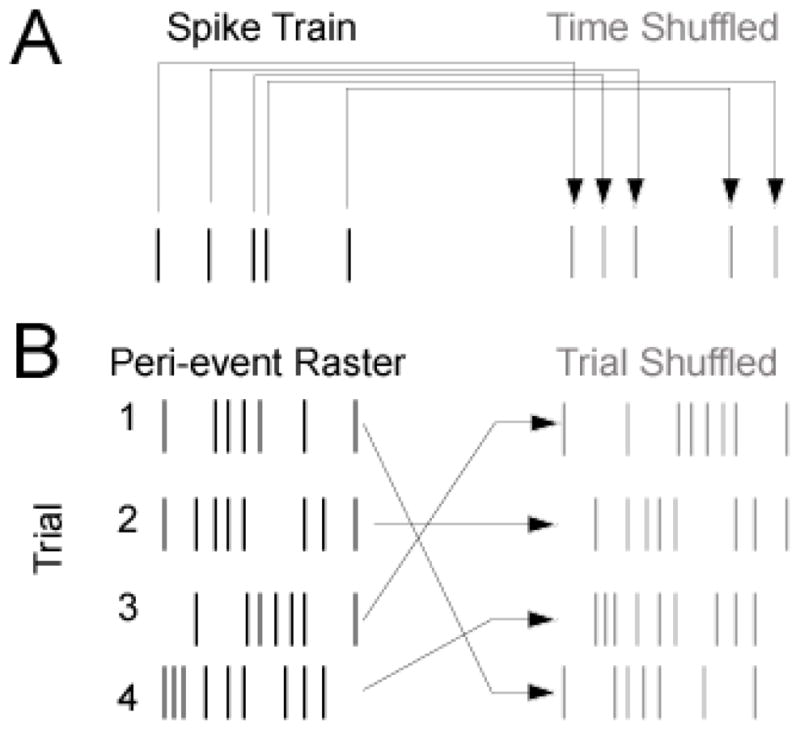
Principles of shuffling can be used to assess empirical significance. A) Time shuffling: in measures of correlation between spike trains, statistical significance can be assessed by comparing data of interest to test statistics generated from time-shuffled data in which spikes are shifted in time. This preserves basic statistics (i.e., firing rate), while destroying temporal information. B) Trial shuffling: in measures of correlation between neurons over trials, statistical significance can be assessed by comparing data of interest to test-statistics generated from trial-shuffled data in which spikes from one trial are shifted to another trial. In a ‘shift predictor’, they are shifted by one trial; however, to account for non-stationarities, it is best to simply scramble the trial order. This preserves basic statistics (i.e., peri-stimulus time histograms, firing rate), while destroying trial-by-trial relationships with other neurons and with behavior.
Using shuffling, one might test the significance of a functional interaction by:
Shuffling spike trains in time or in trials
Applying functional interaction analysis of interest to shuffled data
Repeat steps 1 & 2 as many times as computationally feasible, and obtain a distribution of test statistics from functional interaction analysis. Ten or one-thousand iterations are preferable for defining probability distribution; however, even one hundred iterations can establish significance at p < 0.05.
Establish a significance threshold by determining what values can be expected by chance at a probability of less than p < 0.05 (1 in 20; more stringent thresholds can be used as needed).
For instance, if one is interested in correlations in time, one should compare test statistics derived from correlations to test statistics derived from time-shuffled data (Fig 2A). Time shuffling is appropriate to considering spike trains, which are a series of spikes in time recorded by a data acquisition system corresponding to the timing of action potentials. To time-shuffle a spike train, one can simply generate a random series of spikes matched to the length of the spike train of interest. For instance, to generate a spike train 10 s long at 10 Hz:
randSpiketrain = sort(rand(1, 100) * 10); % random timestamps, 10s @ 10 Hz
More sophisticated temporal distributions (Poisson, bursting) can be generated by providing structure to the random data.
Experiments are commonly performed in ‘trials’, wherein a set of conditions is repeated many times while neuronal activity is tracked. In this scenario, trial-by-trial relationships become important in considering functional interaction between neurons; therefore, destroying this relationship for each neuron preserves neurons’ task modulation but decorrelates neurons’ trial-by-trial relationships. If one is interested in correlations over trials, one should compare test statistics derived from functional interaction analysis to test statistics derived from trial-shuffled data (Fig 2B). To trial-shuffle data, spike trains associated with one trial are switched with a randomly selected trial. This process is also readily achieved in MATLAB with the command
randperm:
myData = rand(149, 10); % random peri-event matrix: 149 trials 10 bins
trialShuffledData = myData(randperm(size(myData, 1)), :); %shuffled data
These methods illustrate that data can easily be shuffled in time or with respect to trials. As detailed above, one should repeat shuffles many times, and compare functional interactions of interest with functional interactions derived from trial- or time- shuffled data. When running the same functional interaction analysis over many pairs of neurons, one must consider how to approach multiple comparisons. At a p < 0.05, 1 in 20 interactions will be significant according to chance. One option is to use a simple correction for multiple comparisons (such as the Bonferonni correction). Alternatively, one can compare the number of functional interactions above a significance level to the number expected by chance via a X2 test.
Functional Grouping by Principal Component Analysis
In exploring functional interactions, a first step is to identify neurons with similar response properties. This can be achieved rapidly via techniques such as principal component analysis (PCA), a standard linear transform that uses singular value decomposition to project multivariate data on a series of axes (or components) to minimize their co-variance. To use PCA, one should:
Arrange perievent histograms from neurons of interest into a matrix where rows are neurons, and columns are bins.
Apply SVD to generate components
Determine the variance accounted for by each component
Visualize the components
An excellent review on the mathematical details on PCA is Reyment and Jöreskog (1996). The method has advantages over other linear transformations in that it does not assume basis vectors and is not iterative; rather, its’ basis vectors are derived directly from the dataset. Other linear transforms may be applied and have other advantages.
PCA is based on singular value decomposition, which can be run in MATLAB using the command svd:
randData = rand(49, 10); % random peri-event matrix: 49 neurons 10 bins
[comps, s] = svd(randData’, 0) % SVD of the peri-event matrix
% plot variance accounted for by components
figure; plot(l  ./  sum(l)); xlabel(‘Components’);
figure; hold on; plot(comps(:, 1:3)); xlabel(‘Time(bins)’);
l = diag(s).^2/(size(randData,2)–1); % percent variance of components
scores = randData * comps; % determine scores on each components
figure; imagesc(scores); xlabel(‘Neurons’); colorbar; % visualize scores
Note the above example is based on randomly generated data simulating a peri-event matrix of 49 neurons over 10 bins. The svd command outputs the components. A key portion of PCA is that the results are easily interpretable in terms of variance when the variance is uniform across the data; for these reasons, it is ideal to work with data normalized to unit variance (i.e., Z scores, where one unit equals one unit of standard deviation; not used above for simplicity).
A scree plot of the variance represented by each component (the variable ‘l’) above is instructive in guiding further analysis. Each number in this variable corresponds to a component; the raw value indicates how many neurons have variance explained by a particular component. Components that are interesting must account for significant variance. One rule of thumb is to extrapolate a line based on lower components; components that fall above this line are of interest; components near this line should be ignored. If desired, more stringent statistical criteria can be used for this determination. The larger the data, the more components may be of interest; however, rarely are more than 5–7 components of further interest. In random data, there is usually only one component (a flat line) that meets these criteria.
One can plot the components with the hope of interpreting them. Using this approach, we identified common response properties across our ensemble by performing PCA on the peri-stimulus time histograms of our recorded neurons in dmPFC and motor cortex. Common forms of variance might correspond to functional groups of neurons within our ensemble.
Finally, the ‘scores’ of each principal component on particular neurons can be computed by matrix multiplying the components by the original data. By restricting components based on variance, dramatic dimension reduction can occur; for instance, in random data, where one component explains >90% of variance, one can go from the original data of 490 values (10 bins X 49 simulated neurons) to 49 values (1 component X 49 neurons), a 90% reduction. The speed and performance of classification and clustering algorithms are improved by such dimension reduction.
We performed principal component analysis on neural data from prefrontal and motor cortices during delayed-response performance. When plotting the variance from each component, we noted that only 3–4 components were large, or greater than a straight line drawn from the smaller components (Fig 3A).
Figure 3.
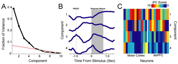
Functional groups identified by principal component analysis (PCA). After peri-stimulus time histograms are extracted, PCA is run to generate a series of components that minimize variance. A) Scree-plot fraction of variance explained by each component. Statistical methods or line-fitting can be used to determine significant components in an automated way; here, we selected 4 components by eye. B) Components as a function of time plotted over the trial in relation to stimulus onset on correct trials only. Note that lever press happens 1.0 s prior to the stimulus, lever release occurs 0–0.6 seconds after the stimulus (mean 0.28 s), and reward acquisition occurs 0.1 s after lever release. Component 1 seems to be response-related; component 2 seems to be related to holding the lever down; component 3 seems to be related to lever press and release movements, and component 4 seems to be involved in stimulus anticipation. C) Components projected onto recorded neurons from motor cortex and dmPFC. Note that strong components (>10) tend to occur on multiple neurons, suggesting common response properties across the population. Absolute value plotted – we are interested in only the strength of the scores.
The components isolated represented behavioral modulations. For instance, component 1 (inverted for clarity) had a large modulation related to responding, component 2 was related to holding the lever down, component 3 was modulated during pressing and releasing the lever, and component 4 was modulated in anticipation of the stimulus (Fig 3B). The sign of a given PC carries information about the relative increases or decreases of firing rates by specific subsets of neurons. However, here we were not interested in this point. Instead, we focused on the issue of whether neurons had similar patterns of activity (i.e., similar changes in firing rates around the behavioral events). Therefore, in this example we discarded the sign of the components.
To determine if there are functional classes within our data set, we examined the projection of PCA scores onto the neurons we recorded. For instance, neuron 1 in motor cortex has a large score for PC4 only (Fig 3C) and therefore is likely involved in motor anticipation. To determine which scores were statistically significant, components were extracted from time-shuffled data. A principal component score of |9.8| corresponded to a p <0.05. Therefore, we interpret scores above this value as significant. We found that 11 neurons had significant projections of component 1 (6 in motor cortex, 5 in dmPFC), 8 neurons had significant projections of component 2 (3 in motor cortex, 5 in dmPFC) and 2 neurons had significant projections of component 3 and 4 (Fig 3C).
PCA is a user-friendly and data-driven tool for exploration of multivariate data. However, there are several potential pitfalls regarding its use. First, the data set must be clean of artifacts (e.g., solenoids) and inconsistent spike sorting across channels can limit the interpretation of PCA. Second, the amount of variance accounted for by components must always be considered. With large data sets, it is tempting to consider smaller components (i.e., ~5). However, only a few neurons usually contribute to such components and we have found that such components are seldom informative about behavior. Third, caution must be applied in interpreting the components, in that the activity of a small subset of neurons at any given moment might drive a given component. To determine the robustness of the components, one should examine the scores for each component and check them against raw plots of neuronal activity, especially for neurons that have large weights on the components. In addition, we recommend that cross-validation techniques be used to assess the overall strength of components. Fourth, components themselves may not be truly orthogonal and methods for rotating the components, such as varimax or ICA, might be useful for interpretation (Laubach et al., 1999).
These concerns notwithstanding, this section illustrates how PCA can readily be used to identify common response properties among a group of simultaneously recorded neurons. Furthermore, these common response properties might correspond to functional groupings among neurons. While identifying patterns of responses, PCA cannot comment on specific interactions between neurons. To make such inferences, we move to other techniques.
Cross-correlation
In neuroscience, a common and readily interpretable measure of functional interactions between neurons is cross-correlation (Aertsen and Gerstein, 1985; Perkel et al., 1975). This method has been used in many neural systems to make powerful inferences about functional interactions as well as functional anatomy. Cross-correlation is designed to make inferences about synaptic connectivity between neurons. In investigating synaptic connectivity, one should observe narrow peaks (a few ms) in the latency of spikes of one neuron with respect to another. If such a peak is observed, then one can potentially make inferences about the number of synapses between each neuron. In certain, highly anatomically connected systems that are guided by topography (such as the auditory system), cross-correlation may provide detailed information about anatomical connectivity in lieu of intracellular recordings. Cross-correlation can also be applied to make inferences about local circuits (Constantinidis et al., 2001). Such inferences must be made with great care and requires having well sorted single units. In extracellular recordings, waveforms recorded on the same wire may interact, diminishing the ability to spike sort. Furthermore, the recording system must sample at high rates to ensure waveforms do not collide. For these reasons, in our group we are hesitant to perform cross-correlative analysis between two neurons on the same wire.
To perform cross-correlations between spike trains from two neurons, one should:
Bin two spike trains of interest at 1 ms bins
Select one spike train as a reference spike train. For each spike in this spike train, determine the time latencies of spikes in the reference spike train to spikes of the other spike train. Typically, time latencies larger than ~200 ms are not of interest for synaptic interactions, greater than 200 ms may indicate slower interactions.
Once latencies are collected, the cross-correlation is simply the histogram of latencies.
To establish significance, peaks obtained in the cross-correlation of interest should be compared with peaks derived from time-shuffled data.
Cross-correlation measures the distance in time between the spikes of one neuron and the spikes of another neuron. If the spikes of one neuron tend to occur at a fixed time relative to the spikes of another neuron, a peak in the cross-correlogram should occur. Though the algorithm is simple, it is computationally intensive, and in MATLAB, relies on the compiled function
xcorr:
t1 = sort(rand(1, 100) * 10); % random timestamps, 10s @ 10 Hz
t2 = sort(rand(1, 100) * 10); % random timestamps, 10s @ 10 Hz
edges = 0:0.001:10;    % 1 ms bins
t1_binned = histc(t1, edges); % timestamps to binned
t2_binned = histc(t2, edges); % timestamps to binned
xc = xcorr(t1_binned, t2_binned); % actual cross-correlation
xc = xc(round(length(xc)/2)-200:round(length(xc)/2)+200);
In the above sample code, two random spike trains are generated lasting 10 s long, firing at approximately 10 Hz. In order for the cross-correlation to be performed, the spike trains must be binned; 1 ms bins is standard for visualizing short-latency synaptic interactions. In MATLAB, histc is a compiled routine that rapidly bins data. The xcorr command computes the cross-correlation. As we are interested only in short latency interactions, the cross-correlation is only kept at latencies +/− 200 ms.
Though the algorithm is simple, this process is computationally intensive. For sessions from behaving animals (tens of minutes to hours), it is preferable to select epochs of interest on the order of tens of seconds for cross-correlation analysis. This selection helps in both computing the random cross-correlation, and in determining confidence intervals via time shuffling.
We performed cross-correlation analysis on neural data from prefrontal and motor cortices during delayed-response performance. In our example data set of 21 neurons, we find rare evidence for synaptic interactions in rodent frontal cortex. One pair of dmPFC neurons had a peak and a trough at 2–4 ms (3B and C), hinting that this pair of neurons are monosynaptically connected or driven by common input. An examination of their response properties reveals that both cells become inhibited as animals initiate lever presses, and stay inhibited until after responses are complete and reward acquisition begins. These interactions provide a glimpse of how information might flow through the rodent dmPFC.
To determine which neurons had significant cross-correlation peaks, we calculated cross-correlation functions from time-shuffled data and compared the ratios of peak sizes for the observed and shuffled data sets. This procedure produced a single metric for the analyses of significant correlations (Fig 5E). For shuffled data, the ratio of peak size of 1.1 corresponded to a p <0.05. We interpreted ratios larger than this to be significant. A total of 35 pairs had significantly larger peaks than could be expected by chance. However, few of these pairs had strong correlations (mean peak to noise ratio: 1.23) (Fig 3E).
Figure 5.

Joint peri-stimulus time-histogram analysis. A) For each trial, spike trains from one neuron are arranged on one axis, and spikes from another neuron are arranged on the orthogonal (i.e., vertical) axis. Coincident spikes over the course of the trial are recorded in the JPSTH matrix. This is repeated for every trial. B) To correct for coincident spikes related to simple modulations in firing rate, the shift predictor is subtracted from the raw JPSTH, and the entire quantity is normalized to units of the shift-predictor (by dividing by the standard deviation of the product of standard deviations of PSTHs). Finally, the JPSTH matrix is compared with an identical matrix computed from trial-shuffled data. C) JPSTH for two motor cortex neurons reveals strong interactions prior to presentation of the stimulus. D) JPSTH peaks across the ensemble.
When using the cross-correlations, several caveats must be considered. The first is that cross-correlation assumes stationarity of neurons. Under typical experimental conditions, many non-stationarities are present (anesthesia state, behavioral motivation, unit waveform drift, satiety states). Secondly, changes in rate can lead to spurious rate correlations – for this reason, a ‘shift-predictor’, i.e., the spike train from one neuron is shifted by the distance of one trial in time, is often subtracted from the cross-correlations to differentiate true interactions from simply rate covariations. Thirdly, in cross-correlative analyses, a sufficient number of spikes in both spike trains are required for statistical inference (Gerstein 1985). Fourthly, as discussed above, cross-correlation inferences rely on clear, artifact-free unit isolation. Fifth, the time-scale of neuronal interactions may influence the cross-correlation (Brody, 1998).
Cross-correlation can also be used to look at long timescale interactions, i.e., on the order of several milliseconds or tens of seconds. Such long timescale interactions do not represent synaptic interactions; rather, they represent an increased between the firing rates of two neurons. While interesting, other techniques (such as rate correlations) may be better suited to such interferences.
These results illustrate how cross-correlation can be used to make inferences about connectivity in multi-electrode data. While this approach is perhaps the most common to studying functional interactions, the cross-correlation does not incorporate how correlations change as a function of behavior. To apprehend the dynamics of correlation, we use the joint-peristimulus time histogram.
Joint-peristimulus time histogram
Since behavior provides a key window into neural responses (via peri-event or peri-stimulus histograms), it is of great interest to know how relationships between neurons vary as a function of stimuli or events. Aertsen and colleagues (Aertsen et al., 1989) created the joint-peristimulus time histogram (JPSTH) for this type of analysis. The JPSTH has been used to investigate relationships between neurons (Vaadia et al., 1988) and areas (Narayanan and Laubach, 2006). In many experiments, the same sequence of events is typically repeated for several ‘trials’. It is interesting to know, then, how correlations between neurons relate to these events. Essentially, the JPSTH analysis looks at time-varying correlation between the neurons relative to stimuli or events.
To perform the JPST analysis, one should:
Arrange the spike trains for two neurons of interest into peri-event matrices; that is, a matrix in which rows are trials, and columns are bins (i.e., 25 ms) bins. Typically for JPSTH analysis, one is not interested in fast interactions; therefore, larger bin sizes (>10 ms) are preferred.
For each trial, record the bin in which spikes occurred for each neuron. A cartesian matrix can then be constructed in which the x axis are bins in which spikes occurred for neuron 1, and y axis are bins in which spikes for neuron y.
Over all the trials in the behavioral session, this cartesian matrix can be summed to generate a joint-peristimulus time matrix. This matrix is referred to as the raw matrix.
It is important to correct for simple modulations in firing rate; to make this correction, perform steps 1–3 for peri-event matrices in which trial orders are shuffled (preferred) or the trials are shifted by one trial. The matrix from these shuffled data are the shift predicted matrix.
Subtract the shift-predicted matrix from the raw matrix.
To compare between neurons, normalization is required. By dividing by the product of standard deviations of the peri-stimulus time histograms of each neuron, one can normalize the JPST matrix to units of correlation.
The two diagonals provide interesting data. The 45-degree diagonal provides a measure of time-varying correlation (also referred to as a correlation time histogram, or CTH), while the perpendicular diagonal (135 degrees) provides a measure of cross-correlation.
As this analysis is a standard technique and is readily performed by existing software packages (NeuroExplorer; Nex Technologies, Littleton, MA; also available from http://mulab.physiol.upenn.edu/) and discussed in detail in the literature (Fig 4A and B) (Aertsen et al., 1989). Here we provide a brief sample of code to calculate the raw matrix:
Figure 4.

Cross-correlation analysis between neurons in multi-electrode data. A) In cross-correlation, for each spike train, the distance (in time) to every other spike of another spike train is recorded, and then a histogram constructed of distances in time of one spike in relation to another spike. B) and C) Peri-stimulus rasters for two dmPFC neurons; both neurons become inhibited prior to lever press, and recover firing rates after the lever is released. D) These neurons have a strong, monosynaptic connection ~2–4 ms, suggesting they are connected or coactivated. These neurons are ~250 um distant. E) Cross-correlation across our ensemble of dmPFC and motor cortex neurons; the ratio of cross-correlation peaks to peaks in trial-shuffled data are plotted (this metric is used to rapidly look across a population of cells). Note there are few strong cross-correlations.
trials = 50; bins = 100; % 50 trials, 100 bins
data1_binned = round(rand(trials, bins)); %sample random data
data2_binned = round(rand(trials, bins)); %sample random data
rawMatrix = zeros(bins, bins); %% preallocate matrices;
data1_hist = zeros(1, bins); data2_hist = data1_hist;
%% for loop to increment through trials
for i = 1:trials;
    x = find(data1_binned(i,:)>0); % find where spikes are
    y = find(data2_binned(i,:)>0); % find where spikes are
   % finds matches and sums the raw matrix where spikes are
     for j = 1:length(x); for k = 1:length(y);
     rawMatrix(x(j),y(k)) = rawMatrix(x(j), y(k))...
         + data1_binned(i, x(j))+data2_binned(i, y(k))–1;
     end; end;
   % increments the PSTH
     data1_hist(x) = data1_hist(x) + data1_binned(i, x);
     data2_hist(y) = data2_hist(y) + data2_binned(i, y);
end
imagesc(rawMatrix); axis xy;
In above code, random data are generated. The loops then increments through the random data to find matches and to generate the raw JPSTH matrix. An optimized version of this approach would avoid for loops; this code is only used for clarity. Also, in order interpret the results, one must subtract a shift-predicted matrix, and divide by the product of standard deviations of PSTHs to normalize the matrix and compare between pairs.
A thorny problem is determination of significance of JPSTH arrays. Established approaches (Aertsen et al., 1989) assess significance either by determine if the modulation can be assessed by chance using a metric referred to as ‘surprise’. We prefer a statistical approach with trial-shuffled data. In this approach, the CTH is calculated both for neurons of interest and for several iterations of trial-shuffled data. One can then investigate whether CTH values observed over a time epoch can be expected due to chance at a p value of 0.05.
An examples of neurons with a significant JPST interaction is shown in Fig 4C. This pair of motor cortex neurons reveals strong negative interactions both along the diagonal as well negative interactions before presentation of the stimulus (meaning that if the horizontal unit is firing, the vertical unit is not), and then a switch during the delay period when the vertical unit fires up to 2 seconds after delay activity in the horizontal unit. The cross-correlation reveals slow interactions on the order of 50–100 ms. these data suggest that there are slow functional interactions between neurons.
We applied this analysis to the neurons in dmPFC and motor cortex in our example data set. In trial-shuffled data, JPSTH values of greater than |0.2| corresponded to p < 0.05 (Narayanan et al., 2006). Pairs of neurons in which one neuron did not have enough spikes (<10 times the number of trials) and from the same wires were excluded. Of 78 potential pairs, 15 (19%) had significant JPST interactions around the time of the stimulus (Fig 4D), 9 in motor cortex, 2 in dmPFC, and 4 between motor and dmPFC.
Several potential pitfalls must be considered when using JPSTH. Foremost, all of the concerns of cross-correlation, including sufficient spikes and non-stationarity, apply when considering JPSTH. Non-stationarities become even more relevant because a confounding variable such as behavioral motivation may create spurious trial-by-trial relationships. The influence of such non-stationarities on JPSTH analysis is unknown. Our experience has been that the JPSTH should be normalized to facilitate comparisons with other neuronal pairs and that bin size is critical, and should be thoroughly explored for each data set of interest.
On the other hand, JPSTH is a flexible technique. Events need not be behavioral; they may be in reference to a third neuron or area (Paz et al., 2006), and even continuous signals might be used in this analysis. Thus JPSTH is a standard way for assessing functional interactions by examining the dynamics of correlations. Both cross-correlation and JPSTH lend themselves to pair-wise analysis of simultaneously recorded neurons.
Rate Correlations
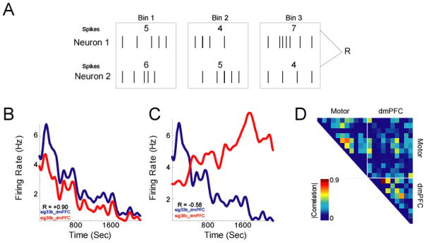
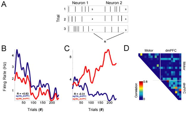
Neurons may show correlations in firing rates in the absence of shared connections (Vaadia et al. 1995; Narayanan and Laubach 2006). Such interactions could occur over time (within trials) or over trials (within bins). Either of these types of functional interactions might correspond to functional units in the nervous system, such as cell assemblies (Tsukada et al., 1996). Because spike trains are point processes, to compute correlations between them one must convert them to a time series by binning (rate correlations / peri-event analyses) (Fig 5A). To compute rate correlations:
Bin two raw spike trains of interest into a series of bin counts
Compute Pearson’s correlation coefficient of binned firing rates
Compare with what might be expected from random data
The above steps are simple and can be rapidly computed:
t1 = sort(rand(1, 200) * 10); % random timestamps,10s @ 20 Hz
t2 = sort(rand(1, 50) * 10); % random timestamps, 10s @ 5 Hz
edges = [0.25:0.25:10]; % edges for 50 ms bins
rate_t1 = histc(t1, edges); % bins for t1
rate_t2 = histc(t2, edges); % bins for t2
scatter(rate_t1, rate_t2); corrcoef(rate_t1, rate_t2)
In the above code, two spike trains are generated, binned, and then correlated. This is a rapid way to look for relationships between the firing rates of two neurons; and also can be useful in addressing non-stationarities that may threaten cross-correlation or JPSTH analyses.
We applied simple rate correlations to dmPFC and motor cortex recordings. We binned spike trains over 10 s over the 39 minutes animals were behaving, resulting in binned firing rates over a total of 235 bins. Note that over this epoch, considerable behavioral fluctuations could occur; however, for the present, we are only interested in relationships between neurons, and ignore all other parameters. In trial shuffled data, correlations greater than |0.14| corresponded to p < 0.05. Of 210 interactions, 109 pairs (52%) had significant rate correlations (67% of dmPFC pairs, 52% of motor cortex pairs, and 45% of dmPFC-motor pairs). Neurons could exhibit strong covariations over the session. For instance, two neurons could be strongly correlated (Fig 5B) or anti-correlated (Fig 5C) over the session. Most neurons did not have strong correlations (Fig 5D). This result suggests that overall correlations were not governed by gross non-stationarities over behavioral sessions (i.e., degradation of unit isolation, artifacts in recording, decline in motivation); rather, the structure of correlations between specific pairs suggested that pairs of neurons exhibited strong functional interactions.
Perhaps the largest difficulty with rate correlations is that the animals’ behavior is uncontrolled. Correlations may be driven by behavioral variability, similar functional properties across neurons (compare with PCA), or even task-irrelevant behavior, such as grooming or movement artifacts. For these reasons, it is somewhat difficult to interpret rate correlations, especially in the absence of well-controlled operant behavior. In using rate correlations, all previous caveats apply (unit isolation, sufficient spikes). Furthermore, the number of bins should be carefully chosen. Too few bins lead to inflated correlation coefficients. Too many bins may destroy temporal structure. For this reason, any observed correlation must be explored at a variety of bin sizes.
These methods demonstrate how to use simple rate correlations to make inferences about functional relationships between neurons, and demonstrate how these techniques can be applied to simultaneous recordings from neural populations in rodent dmPFC and motor cortex.
Trial-by-trial rate correlations
In essence, the JPSTH applies cross-correlation on a trial-by-trial basis. Gawne and Richmond (1993) proposed the same analogy for rate correlations. This analysis is simple to calculate, as one can compare (via correlation) the mean or the variance of activity of two neurons over trials (Fig 6A). To perform rate correlation, one should:
Figure 6.
Rate correlations. A) This analysis simply bins neurons’ firing rates over the session, and examines the correlation of neurons’ binned firing rates over time. B) Neurons could exhibit positive or C) negative relationships. D) Rate correlations over the ensemble (absolute value plotted – we are interested in only the strength of correlation) reveal several groups of neurons with strong rate correlations in both areas.
Construct peri-event matrices for each neuron
Sum the firing rates for each trial
Compute Pearson’s correlation coefficient of trial-by-trial firing rates.
These steps also can be easily computed with the following code, in which two peri-event matrices are created from random data, and a correlation coefficient is calculated.
data1 = rand(70, 10); % random peri-event matrix: 70 trials, 10 bins
data2 = rand(70, 10); % random peri-event matrix: 70 trials, 10 bins
fr_data1 = mean(data1′); % sums along rows
fr_data2 = mean(data2′); % sums along rows
scatter(fr_data1, fr_data2); corrcoef(fr_data1, fr_data2)
We applied trial-by-trial rate correlations to our sample dmPFC and motor cortex recordings over 235 correct trials; this number yielded similar power as our rate correlation analysis (above); over each trial, animals performed a stereotyped series of actions. In trial-shuffled data, we found that correlations greater than |0.18| corresponded to p < 0.05. Of 210 interactions, 56 pairs (27%) had significant trial-by-trial rate correlations (69% of dmPFC pairs, 16% of motor cortex pairs, and 43% of dmPFC-motor pairs). Neurons exhibited strong trial-by-trial covariations. For instance, two neurons could be strongly correlated (Fig 6A) or anti-correlated (Fig 6B) over the session; these are the same neurons with rate correlations. Most neurons did not have strong correlations (Fig 6C). Note that while motor cortex neurons had strong rate correlations, they tended not have strong trial-by-trial interactions. These methods, then, are able to separate resolve patterns of functional correlations.
Predictive Interactions
Thus far, we have discussed functional interactions in three domains – patterns of activity (PCA), timing of spikes (cross-correlation / JPSTH) and fluctuations in firing rate (rate and trial-by-trial covariations). Though these approaches are powerful in examining relationship between neurons, none of these approaches examines how neurons predict behavior. If neurons predict behavior in similar ways, then they may have functional interactions that are due to behavior.
To investigate relationships in how neurons predict behavior, we used methods from the field of machine learning, or statistical pattern recognition, to quantify information from spike trains about behavior on a trial-by-trial basis (see Laubach et al., 2007 for review of methods for spike train analysis and Witten and Frank, 2000 and Hastie et al., 2001 for a review of the statistical issues). By comparing the predictions of behavior between two neurons, we can investigate whether neurons predict behavior in the same way (i.e., predict the same behavior on the same trials), or in different ways (i.e., predict behavior as would be expected by chance) (Fig 7A). To perform statistical pattern recognition, one should:
Figure 7.
Trial-by-trial rate correlations. A) This analysis simply bins neurons’ firing rates over the trials, and examines the correlation of neurons’ firing rates over trials. B) Neurons could exhibit positive or C) negative relationships; same neurons as in Fig 6. D) Trial-by-trial rate correlations over the ensemble (absolute value plotted – we are interested in only the strength of correlation) reveal several groups of neurons with strong trial-by-trial correlations, particularly in dmPFC.
Construct peri-event matrices for each neuron
Prepocess the peri-event matrices (smoothing and decimation)
Reduce the dimensions of the data (via PCA or wavelet-based methods). This step is important for optimizing classifier performance; irrelevant dimensions will both slow and decrease classifier performance.
Segment the data into a training data and a testing set
Training a classifier from training data to predict the behavioral outcome of testing data. Repeat at least 10 times (10 fold cross-validation) (Witten and Frank, 2000).
Evaluate classifier performance with information theory or ROC analysis
Repeat steps 1–5 for trial-shuffled data
Implementation of these steps is highly involved and requires careful understanding of the methods used for preprocessing, dimension reduction, and classification. In essence, statistical pattern recognition uses neuronal data to predict a behavioral variable on each trial. Classifier performance can then be quantified by comparing classifier predictions of the behavioral variable (i.e., slow vs. fast RTs) with the actual behavioral variable (the RT that the animal actually made).
Below is a brief demonstration with random data using PCA and k-means clustering:
%make random data; 40 trials, 100 bins, 2 classes
a = rand(40,100); b = rand(40,100) * 1.2; % 1.2 is the separation coeff
data = ([a; b]);
groups = [ones(1,40) ones(1,40)*2]; % make a groups vector
[u, s, v] = svd(data’, 0); % pca for dimension reduction
U = u(:, 1:3); %only first three components
scores = data * U; % obtain scores for PCA
% Use k means to cluster groups in high dimensional space. This is being used
% as a classifier WITHOUT cross validation, and although it is not a strong %
% classifier, it illustrates the point; any classifier will do
[pred1, C] = kmeans(scores, length(unique(groups)));
% Plot the PC scores in dimensional space; check for clusters
g1 = find(groups==1); g2 = find(groups==2); hold on;
scatter3(scores(g1, 1), scores(g1, 2), scores(g1, 3), ‘k.’);
scatter3(scores(g2, 1), scores(g2, 2), scores(g2, 3), ‘r.’);
scatter3(C(:, 1), C(:, 2), C(:, 3), ‘b+’);
confusionMatrix(1, 1)=length((find(pred1(g1)==1)));% true positive
confusionMatrix(1, 2)=length((find(pred1(g1)==2)));% false positive
confusionMatrix(2, 1)=length((find(pred1(g2)==1)));% false negative
confusionMatrix(2, 2)=length((find(pred1(g2)==2)));% true negative
In the above code, random data are created. In one class, a slight bias of 20% (represented by the factor 1.2 above) is generated. PCA is then performed for dimension reduction, and k-means clustering is used for classification. Classification is then assessed using a ‘confusion matrix’, or a 2 X 2 matrix comparing predicted (rows) vs. actual (columns) classification. Note that this approach, with 20% bias, generates relatively robust classification at minimal computational cost.
In our lab, we perform the above analysis somewhat differently (Laubach et al., 2007). We identify correct trials with reaction times in the lower quartile (selected to speed classification; equivalent results are possible for other splits of reaction time, or accuracy) (Narayanan et al., 2005) and construct perievent histograms (using 1 ms bins) for the epoch from 250 ms before lever release to 250 ms after the presentation of the trigger stimulus. The histograms were smoothed, using 10-fold decimation and low-pass filtering, and decomposed into a set of components that were ordered by relative variance. This latter step was carried out using wavelet packet analysis (Laubach, 2004)based on the matching pursuit algorithm (Mallat and Zhang, 1993). A 4-point “symmlet” filter was used for the wavelet packet analysis.
Matching pursuit is a sequential decomposition algorithm that finds a series of signal components (up to 10 in this case) that account for decreasing levels of variance in the average peri-event histograms of each neuron. This step is used in lieu of PCA above (as in Richmond and Optican 1987). This procedure is useful for reducing the complexity (i.e., dimensionality) of the data prior to analysis with statistical classifiers. By using matching pursuit, we reduced the dimensionality of the neuronal spike data, from 400 1-ms bins (the number of bins in a peri-stimulus time histogram) to typically 5 or fewer matching pursuit task-related features. Scores for matching pursuit components are defined from trials with the lower one-fourth of RTs. Scores were calculated as the dot product of the wavelet filter and the measured neuronal firing on each trial. The scores were then used to train statistical classifiers. Regularized discriminant analysis (RDA) (Friedman, 1989) was used with leave-one-out cross-validation to predict trials with fast RTs vs. trials with slow RTS (top quartile).
RDA is a non-parametric form of linear discriminant analysis that is a appropriate for data with non-Gaussian distributions (i.e., the scores from matching pursuit) and that allows for non-linearity in the discriminant functions (Hastier et al., 2001). We normally use such an algorithm in lieu of k-means, which is used in this chapter for explanatory simplicity. Note that in the above sample code, cross-validation is not done; in general, it must be done obtain measures of bias and variance. Results obtained from the classifiers were used to construct ‘confusion matrices’ – i.e., a list of trial outcomes vs. the predictions of trial outcome made by the classifier in the form of a 2×2 table (for a data set with 2 possible outcomes there are 2 rows and columns in the confusion matrix). Whereas PCA and k-means is successful with a ~20% bias, using our approach, we can reliably predict biases of ~10%. However, this approach requires several libraries for the program R (http://cran.r-project.org/) for rapid classification. Examples are available on our website (spikelab.jbpierce.org/Resources) and have been described in detail in previous publications (Naraynan et al., 2005; Laubach et al., 2007).
If neurons have a shared predictive relationship, then they should have shared predictions that are stronger than would be expected in trial-shuffled data. This is readily quantified by the following code:
for i = 1:10000
    pred1 = zeros(1, 100); pred2 = zeros(1, 100);
    pred1(find(rand(1, 100)>0.7))=1; % 70% prediction
    pred2(find(rand(1, 100)>0.6))=1; % 60% prediction
    match(i) = length(find(pred1==pred2));
end
The distribution of the variable match provides a probability distribution that is used to assess the significance of predictions.
We applied this approach to two neurons from dmPFC and motor cortex. Although these two neurons provided small amounts of predictive information (0.005 bits for the motor cortex neuron, 0.03 bits for the dmPFC neuron; Fig 8B), we found that these neurons shared predictions 59% of the time, more than could be expected by chance (44±9%, p < 0.05). These data indicate that neurons that were weakly predictive of behavior could still share predictive relationships.
Figure 8.

Predictive interactions. A) Statistical pattern recognition uses trial-by-trial spike train to generate predictions of behavior on a trial-by-trial basis. These predictions can be compared with predictions from another neuron. B) Peri-stimulus rasters of neurons and their predictions of reaction time; black corresponds to trials with short RTs, red corresponds to trials with slow RTs. In between the peri-stimulus rasters, predictions are plotted: black means that a fast RT was predicted from spike trains; red means that a slow RT was predicted. Central column: green indicates that the two neurons agreed in their predictive information; white indicates that the neurons disagreed. These neurons tended to agree more than could be expected by chance, and thus had an interaction in their predictive information. F) Predictive interactions across the ensemble.
Across our population, we compared neuronal predictions with neuronal predictions from within class (i.e., within fast and with slow RTs) trial-shuffled data (Fig 8C). We found that improvements in classification of 9% over random data corresponded to p < 0.05. We found that 12 (of 127; 10%) predictive interactions were greater than could be expected by chance. We would expect to find this number of significant predictive interactions at p < 0.05 by chance (X2 = 2.15, p < 0.14).
We also compared predictive information on a trial-by-trial basis between dmPFC and motor cortex. The population of 10 dmPFC neurons provided 0.2 bits of information, whereas the population of 11 motor cortex neurons provided 0.5 bits of information. When predicting fast RTs, dmPFC and motor cortex shared predictions (76%) that could be explained by chance (p < 0.05 at 76%). On the contrary, when predicting slow RTs, dmPFC and motor cortex shared predictions (86%) were higher than could be explained by mere correlations with RT (p < 0.05 at 83%).
The use of statistical pattern recognition to explore trial-by-trial relationships in predictions between neurons should be approached carefully. This analysis is complex and reliant on understanding of procedures such as dimension reduction and classification. In pattern recognition, one must also worry about bias and variance (Witten and Frank, 2000), which can readily influence trial-by-trial predictions.
However, these results indicate that dmPFC and motor cortex populations have functional interactions in their trial-by-trial predictive information (that is, their predictions about reaction times) only when predicting slow RTs. This type of analysis suggests that dmPFC neurons and motor cortex neurons functionally interact on slow but not fast RTs. This novel insight is an example of how predictive relationships between populations of neurons can be used to make inferences about how these populations interact.
Network Interactions: Synergy and Redundancy
As an extension of the preceding analyses of shared predictive relationships, one might ask how the predictive information of a two-neuron ensemble compared to the predictive information of each neuron individually. If two neurons provided more information individually than they do together, then they interact redundantly. On the other hand, if they provide more information together than they do individually, then they interact synergistically. This idea provides a framework (Gawne and Richmond, 1993; Narayanan et al., 2005; Schneidman et al., 2003) for interpreting network interactions (Fig 9A)
Figure 9.
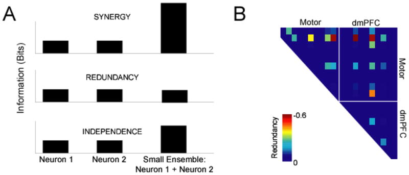
Network interactions. A) Two neurons predictive information can interact to produce more information together than individually (synergy), less information together than individually, or simply the linear sum together of their information individually (independence). B) Redundancy interactions across the ensemble; we observed almost exclusively redundant interactions across the ensemble; note that this analysis is limited only to neurons with significant predictive information.
To assess network interactions, one should:
Construct peri-event matrices for one neuron
Preprocess the peri-event matrices (smoothing and decimation)
Reduce the dimensions of the data (via PCA or wavelet-based methods)
Segment the data into a training data and a testing set
Training a classifier from training data to predict the behavioral outcome of testing data
Repeat steps 1–5 for another neuron
Repeat steps 1–5 for the two neurons together
Compare information of the two neurons together with the information of each neuron individually.
If the predictive information of two neurons were greater than the sum of the predictive information individually, then we would call this a synergistic interaction. On the other hand, if the predictive information of two neurons were less than the sum of the predictive information of each neuron individually, then we would call this a redundant interaction. Finally if the predictive information of two neurons were equal to the sum of the predictive information of each neuron individually, then we would call this an independent interaction.
Again, as with the previous section, the code for the pattern recognition is complex; on the other hand, the computation of whether neurons are synergistic, independent, or redundant is simple (Narayanan et al., 2005):
Where IEnsemble is the predictive information of the ensemble, or two neurons together, and INeuron, is the predictive information of individual neurons in the ensemble.
We applied this analysis to our population of neurons recorded in dmPFC and motor cortex (Fig 9B). First, we found for 36 pairs with predictive information, the mean Pensemble was −0.19 bits, suggesting overall redundant interactions. These results are convergent with previous studies from out lab (Narayanan et al., 2005). We found that a Pensemble of −0.2 corresponded to p < 0.05. According to this metrics, 13 (of 36 pairs; 36%) pairs had significantly redundant interactions.
As an ensemble, we found that the population of neurons in both areas (dmPFC and motor cortex) provided 0.55 bits of predictive information. Motor cortex alone provided 0.5 bits of information, while dmPFC alone provided 0.2 bits of information. Thus combined, both areas had 0.15 bits of redundancy (Pensemble = −0.15), below the significance level. These results suggest a lack of strong synergistic or redundant interactions between dmPFC and motor cortex.
Comparison of Functional Interactions With Multiple Techniques
We have presented an array of techniques for assessing functional interactions in this manuscript. Each technique we have presented describes a different aspect of how neurons interact, and provides a distinct perspective to neurons functional interactions. To provide a multivariate portrait of functional interactions, we present a table describing the interactions between two pairs of neurons (Table 1).
Table 1.
Functional Interactions
| Chance | Pair | Pair | |
|---|---|---|---|
|
|
|||
| - | sig033b_dmPFC sig038b_dmPFC |
sig040a_dmPFC sig024a_MC |
|
|
|
|||
| Principal Component Analysis | 9.8 | Hold component (PC 2) | No common component |
| Cross-correlation | 1.1 | 12 | 1.0 |
| JPSTH | 0.2 | 0 | 0.35 |
| Rate Correlation | 0.14 | 0.91 | −0.03 |
| Trial-by-trial Correlation | 0.18 | 0.83 | 0.17 |
| Predictive Information | ~ | 0.72 | 0.83 |
| Redundancy | −0.2 | −0.002 | −0.46 |
For the first pair of neurons, (sig033b_dmPFC & sig038b_dmPFC), we find similar response properties (holding the lever down) strong cross-correlations (the ratio of peaks to peaks in random noise is shown), suggesting a synaptic relationship. We also find strong rate and trial-by-trial rate correlations; however, we find no instance of JPSTH interactions, predictive interactions, and hence, no network interactions. This type of pair, while interesting to many neuroscientists because it describes a monosynaptically connected pair of neurons at least 250 um distant from each other, has no correlations that change in relation to stimulus presentation and is poorly predictive of reaction time. This is a classic example of a noise correlation (Averbeck et al., 2006), that is, despite the fact that these neurons themselves are having similar behavioral modulations, the communication between this pair of neurons is not directly related to behavior. This pair belies the importance of our approach of comparing correlative techniques, as no one measure of functional interactions provides a complete picture of neuronal interactions.
Another pair of neurons (sig040a_dmPFC and sig030a_MC) in different cortical areas has an opposite pattern. The neurons do not share components, and the cross-correlation, rate-correlation, and trial-by-trial correlation of these neurons is small; however, we find strong JPSTH correlations, predictive interactions, and redundant network interactions. This pair is easily ignored because of a lack of clear cross-correlations or trial-by-trial correlations; nonetheless, this pair has strong JPSTH and predictive relationships. These neurons likely have a strong signal (where signal is controlling response to the stimulus) correlation (Averbeck et al., 2006), in that they seem to be working together to predict behavior. Their functional interactions that may allude to top-down control of dmPFC on motor cortex (Narayanan and Laubach 2006).
Finally, we integrate these analyses to provide a map of functional interactions (Fig 10). In this case, we are not interested in significance; rather, we are interested in patterns of interactions including subthreshold values. For these reasons, we present a scaled correlation map across ensembles of neurons in frontal cortex.
Figure 10.

Integrating functional interactions between measures. A) Interactions within motor cortex B) dmPFC, and between dmPFC and motor cortex using techniques presented in this paper. For comparison, all interactions are normalized within a class of interactions, and presented as absolute value.
We notice that in motor cortex, functional interactions are common at the level of cross-correlation and JPSTH, but rare in rate or predictive interactions. On the contrary, in dmPFC, cross-correlation and JPSTH interactions are rare, but rate or predictive interactions are more common. Between dmPFC and motor cortex particular combinations of neurons seemed to have robust functional correlations. These results demonstrate, in principle, how functional interactions can be combined to elucidate patterns of interaction among cortical networks.
Thus studying different kinds of functional interactions across an ensemble of simultaneously recorded neurons in multi-electrode experiments affords novel insights into how neurons work together to encode information, and provides evidence that neurons can work together in diverse ways in service of behavior.
NOTES
Here we have described seven distinct approaches to investigating functional interactions between neurons: functional grouping by PCA, cross-correlation, joint-peristimulus time histograms, rate correlations, trial-by-trial rate correlations, predictive interactions, and network interactions. We have described how to perform each analysis, limitations and applications of each analysis, and demonstrated how such analysis might work in an ensemble of 21 simultaneously recorded neurons from rodent dmPFC and motor cortex. By integrating and comparing functional interactions, we are able to gain insight on how relationships among populations of neurons contribute to the encoding of behavior.
While we have restricted our analysis of functional interactions to the methods discussed here, many investigators have developed an arsenal of tools with which to assail the problem of neuronal interactions. These include peer-prediction, in which pattern recognition is used to predict the spikes of another neuron (Harris et al., 2003), information theory, in which a ‘lookup table’ is constructed to predict the information in one spike train from another (Schniedemann et al., 2003), detection of synchrony (Gray et al., 1992), coherence (both in spike and field), in which frequency relationships between field potential and spikes from different channels are used to make inferences about local and distant processing (Pesaran et al., 2002), as well as a host more under current development. Each of these techniques has strengths and pitfalls, and may be able to be readily applied to our data. However, though we have limited our discussion to several readily applicable and relatively simple techniques that demonstrate the principles of considering functional interactions between neurons, we recognize that future analyses using the techniques above or still being developed may further refine or expand our interpretations of how neurons interact.
What is the significance of the functional interactions described here? Averbeck and colleagues have examined correlated variability between neurons (Averbeck et al., 2003; Averbeck and Lee, 2003; Averbeck and Lee, 2004; Averbeck and Lee, 2006). They mention two ideas when considering neuronal correlations: signal correlations, i.e., correlations that relate to an outside, measured variable, and noise correlations, i.e., correlations that do not relate to any measured variable. Some investigators have suggested that such noise correlations play a crucial role in neural processing (Gray et al., 1992). Trial-shuffling plays a key role in discriminating between signal and noise correlations (Averbeck et al., 2006), and is analogous to the within-class trial shuffling performed in our analysis of predictive information to determine if shared predictive relationships were related to high predictive information (signal correlations) or to shared predictive relationships (noise correlation). Furthermore, we report neurons with high noise and low signal correlations (Table 1, 1st column) as well as neurons with high signal and noise correlations (Table 1, 2nd column). However, such analyses typically require robust measurement of signal via a tuning curve; our task is too simple for such an analyses. Instead, we focus on using multiple approaches to develop a picture of neural interactions.
In exploring functional correlations between neurons, one must remember the anatomy of the brain areas of interest. For example, when recording between distinct cortical areas, one must understand the probability of direct synaptic connections, and shared inputs. Furthermore, it is helpful to know in which other areas the neurons might interact (i.e., thalamus), and whether in other brain areas, projections to the neurons originate from the same neurons. While this information is difficult to get and requires painstaking anatomy, it is critical to interpreting data about how neurons interact. Within a cortical area, columnar organization, laminar information, receptive field properties, and recurrent connectivity all will help define and constrain interpretation of functional interactions between simultaneously recorded neurons (Mountcastle, 1998; Shepherd, 2003).
Finally, the goal of studying functional interactions is to design clear experiments that test hypothesis about how neurons interact. For instance, we combined JPSTH analyses with techniques that inactivate dmPFC while recording from motor cortex to make insights about how the two areas might interact (Narayanan et al., 2006). One could imagine future studies targeting microstimulation to groups with strong functional interactions, and investigate the role of stimulation of one neuron on some other (distant neuron). Experiments of this nature will provide novel insights on how cortical neurons work together to control behavior.
Acknowledgments
We thank Eyal Kimchi and Nicole Horst for critical comments and helpful discussions. This work was supported by funds from the Tourette Syndrome Association, Kavli Institute at Yale, and the John B. Pierce Laboratory for ML and from an NIH training grant to the Yale Medical Scientist Training Program and Army Research Office for NSN.
References
- Aertsen AM, Gerstein GL. Evaluation of neuronal connectivity: sensitivity of cross-correlation. Brain Res. 1985;340:341–354. doi: 10.1016/0006-8993(85)90931-x. [DOI] [PubMed] [Google Scholar]
- Aertsen AM, Gerstein GL, Habib MK, Palm G. Dynamics of neuronal firing correlation: modulation of “effective connectivity”. J Neurophysiol. 1989;61:900–917. doi: 10.1152/jn.1989.61.5.900. [DOI] [PubMed] [Google Scholar]
- Averbeck BB, Crowe DA, Chafee MV, Georgopoulos AP. Neural activity in prefrontal cortex during copying geometrical shapes. II. Decoding shape segments from neural ensembles. Exp Brain Res. 2003;150:142–153. doi: 10.1007/s00221-003-1417-5. [DOI] [PubMed] [Google Scholar]
- Averbeck BB, Latham PE, Pouget A. Neural correlations, population coding and computation. Nat Rev Neurosci. 2006;7:358–366. doi: 10.1038/nrn1888. [DOI] [PubMed] [Google Scholar]
- Averbeck BB, Lee D. Neural noise and movement-related codes in the macaque supplementary motor area. J Neurosci. 2003;23:7630–7641. doi: 10.1523/JNEUROSCI.23-20-07630.2003. [DOI] [PMC free article] [PubMed] [Google Scholar]
- Averbeck BB, Lee D. Coding and transmission of information by neural ensembles. Trends Neurosci. 2004;27:225–230. doi: 10.1016/j.tins.2004.02.006. [DOI] [PubMed] [Google Scholar]
- Averbeck BB, Lee D. Effects of noise correlations on information encoding and decoding. J Neurophysiol. 2006;95:3633–3644. doi: 10.1152/jn.00919.2005. [DOI] [PubMed] [Google Scholar]
- Britten KH, Newsome WT, Shadlen MN, Celebrini S, Movshon JA. A relationship between behavioral choice and the visual responses of neurons in macaque MT. Vis Neurosci. 1996;13:87–100. doi: 10.1017/s095252380000715x. [DOI] [PubMed] [Google Scholar]
- Brody CD. Slow covariations in neuronal resting potentials can lead to artefactually fast cross-correlations in their spike trains. J Neurophysiol. 1998;80:3345–3351. doi: 10.1152/jn.1998.80.6.3345. [DOI] [PubMed] [Google Scholar]
- Carmena JM, Lebedev MA, Crist RE, O’Doherty JE, Santucci DM, Dimitrov D, Patil PG, Henriquez CS, Nicolelis MA. Learning to control a brain-machine interface for reaching and grasping by primates. PLoS Biol. 2003;1:E42. doi: 10.1371/journal.pbio.0000042. [DOI] [PMC free article] [PubMed] [Google Scholar]
- Constantinidis C, Franowicz MN, Goldman-Rakic PS. Coding specificity in cortical microcircuits: a multiple-electrode analysis of primate prefrontal cortex. J Neurosci. 2001;21:3646–3655. doi: 10.1523/JNEUROSCI.21-10-03646.2001. [DOI] [PMC free article] [PubMed] [Google Scholar]
- Dan Y, Alonso JM, Usrey WM, Reid RC. Coding of visual information by precisely correlated spikes in the lateral geniculate nucleus. Nat Neurosci. 1998;1:501–507. doi: 10.1038/2217. [DOI] [PubMed] [Google Scholar]
- Friedman J. Regularized discriminant analysis. Journal of American Statisical Association. 1989;84:166–175. [Google Scholar]
- Gawne TJ, Richmond BJ. How independent are the messages carried by adjacent inferior temporal cortical neurons? J Neurosci. 1993;13:2758–2771. doi: 10.1523/JNEUROSCI.13-07-02758.1993. [DOI] [PMC free article] [PubMed] [Google Scholar]
- Gochin PM, Colombo M, Dorfman GA, Gerstein GL, Gross CG. Neural ensemble coding in inferior temporal cortex. J Neurophysiol. 1994;71:2325–2337. doi: 10.1152/jn.1994.71.6.2325. [DOI] [PubMed] [Google Scholar]
- Gray CM, Engel AK, Konig P, Singer W. Synchronization of oscillatory neuronal responses in cat striate cortex: temporal properties. Vis Neurosci. 1992;8:337–347. doi: 10.1017/s0952523800005071. [DOI] [PubMed] [Google Scholar]
- Harris KD, Csicsvari J, Hirase H, Dragoi G, Buzsaki G. Organization of cell assemblies in the hippocampus. Nature. 2003;424:552–556. doi: 10.1038/nature01834. [DOI] [PubMed] [Google Scholar]
- Hastie T, Tibshirani R, Friedman J. The Elements of Statistical Learning. New York, NY: Springer-Verlag; 2001. [Google Scholar]
- Laubach M. Wavelet-based processing of neuronal spike trains prior to discriminant analysis. J Neurosci Methods. 2004;134:159–168. doi: 10.1016/j.jneumeth.2003.11.007. [DOI] [PubMed] [Google Scholar]
- Laubach M, Narayanan NS, Kimchi EY. Single-neuron and ensemble contributions to decoding simultaneously recorded spike trians. In: Holscher C, editor. Neuronal population recordings. 2007. [Google Scholar]
- Laubach M, Shuler M, Nicolelis MA. Independent component analyses for quantifying neuronal ensemble interactions. J Neurosci Methods. 1999;94:141–154. doi: 10.1016/s0165-0270(99)00131-4. [DOI] [PubMed] [Google Scholar]
- Laubach M, Wessberg J, Nicolelis MA. Cortical ensemble activity increasingly predicts behaviour outcomes during learning of a motor task. Nature. 2000;405:567–571. doi: 10.1038/35014604. [DOI] [PubMed] [Google Scholar]
- Mallat S, Zhang Z. Matching pursuits with time-frequency dictionaries. IEEE Transactions. 1993;41:3397–3415. [Google Scholar]
- Mountcastle VB. Perceptual Neuroscience: The Cerebral Cortex. Cambridge, MA: Harvard College; 1998. [Google Scholar]
- Narayanan NS, Horst NK, Laubach M. Reversible inactivations of rat medial prefrontal cortex impair the ability to wait for a stimulus. Neuroscience. 2006 doi: 10.1016/j.neuroscience.2005.11.072. [DOI] [PubMed] [Google Scholar]
- Narayanan NS, Kimchi EY, Laubach M. Redundancy and synergy of neuronal ensembles in motor cortex. J Neurosci. 2005;25:4207–4216. doi: 10.1523/JNEUROSCI.4697-04.2005. [DOI] [PMC free article] [PubMed] [Google Scholar]
- Narayanan NS, Laubach M. Top-down control of motor cortex ensembles by dorsomedial prefrontal cortex. Neuron. 2006;52:921–931. doi: 10.1016/j.neuron.2006.10.021. [DOI] [PMC free article] [PubMed] [Google Scholar]
- Nicolelis MA, editor. Methods In Neuronal Ensemble Recording. Boca Raton, FL: CRC Press; 1998. [Google Scholar]
- Nicolelis MA, Ghazanfar AA, Stambaugh CR, Oliveira LM, Laubach M, Chapin JK, Nelson RJ, Kaas JH. Simultaneous encoding of tactile information by three primate cortical areas. Nat Neurosci. 1998;1:621–630. doi: 10.1038/2855. [DOI] [PubMed] [Google Scholar]
- Paz R, Pelletier JG, Bauer EP, Pare D. Emotional enhancement of memory via amygdala-driven facilitation of rhinal interactions. Nat Neurosci. 2006;9:1321–1329. doi: 10.1038/nn1771. [DOI] [PubMed] [Google Scholar]
- Perkel DH, Gerstein GL, Smith MS, Tatton WG. Nerve-impulse patterns: a quantitative display technique for three neurons. Brain Res. 1975;100:271–296. doi: 10.1016/0006-8993(75)90483-7. [DOI] [PubMed] [Google Scholar]
- Pesaran B, Pezaris JS, Sahani M, Mitra PP, Andersen RA. Temporal structure in neuronal activity during working memory in macaque parietal cortex. Nat Neurosci. 2002;5:805–811. doi: 10.1038/nn890. [DOI] [PubMed] [Google Scholar]
- Reich DS, Mechler F, Victor JD. Independent and redundant information in nearby cortical neurons. Science. 2001;294:2566–2568. doi: 10.1126/science.1065839. [DOI] [PubMed] [Google Scholar]
- Reyment R, Jöreskog KG. Applied factor analysis in the natural sciences. Cambridge University Press; 1996. [Google Scholar]
- Richmond BJ, Optican LM. Temporal encoding of two-dimensional patterns by single units in primate inferior temporal cortex. II. Quantification of response waveform. J Neurophysiol. 1987;57:147–161. doi: 10.1152/jn.1987.57.1.147. [DOI] [PubMed] [Google Scholar]
- Rolls ET, Aggelopoulos NC, Franco L, Treves A. Information encoding in the inferior temporal visual cortex: contributions of the firing rates and the correlations between the firing of neurons. Biol Cybern. 2004;90:19–32. doi: 10.1007/s00422-003-0451-5. [DOI] [PubMed] [Google Scholar]
- Rolls ET, Treves A, Tovee MJ. The representational capacity of the distributed encoding of information provided by populations of neurons in primate temporal visual cortex. Exp Brain Res. 1997;114:149–162. doi: 10.1007/pl00005615. [DOI] [PubMed] [Google Scholar]
- Schneidman E, Bialek W, Berry MJ., 2nd Synergy, redundancy, and independence in population codes. J Neurosci. 2003;23:11539–11553. doi: 10.1523/JNEUROSCI.23-37-11539.2003. [DOI] [PMC free article] [PubMed] [Google Scholar]
- Shepherd G. Synaptic Organization of The Brain. 34. Oxford: Oxford University Press; 2003. [Google Scholar]
- Tsukada M, Ichinose N, Aihara K, Ito H, Fujii H. Dynamical Cell Assembly Hypothesis - Theoretical Possibility of Spatio-temporal Coding in the Cortex. Neural Netw. 1996;9:1303–1350. [PubMed] [Google Scholar]
- Vaadia E, Haalman I, Abeles M, Bergman H, Prut Y, Slovin H, Aertsen A. Dynamics of neuronal interactions in monkey cortex in relation to behavioural events. Nature. 1995;373:515–518. doi: 10.1038/373515a0. [DOI] [PubMed] [Google Scholar]
- Vaadia E, Kurata K, Wise SP. Neuronal activity preceding directional and nondirectional cues in the premotor cortex of rhesus monkeys. Somatosens Mot Res. 1988;6:207–230. doi: 10.3109/08990228809144674. [DOI] [PubMed] [Google Scholar]
- Vaadia E, Haalman I, Abeles M, Bergman H, Prut Y, Slovin H, Aertsen A. Dynamics of neuronal interactions in monkey cortex in relation to behavioural events. Nature. 1995;373:515–518. doi: 10.1038/373515a0. [DOI] [PubMed] [Google Scholar]
- Wessberg J, Stambaugh CR, Kralik JD, Beck PD, Laubach M, Chapin JK, Kim J, Biggs SJ, Srinivasan MA, Nicolelis MA. Real-time prediction of hand trajectory by ensembles of cortical neurons in primates. Nature. 2000;408:361–365. doi: 10.1038/35042582. [DOI] [PubMed] [Google Scholar]
- Witten I, Frank E. Data Mining. San Diego, CA: Academic Press; 2000. [Google Scholar]
- Zohary E, Shadlen MN, Newsome WT. Correlated neuronal discharge rate and its implications for psychophysical performance. Nature. 1994;370:140–143. doi: 10.1038/370140a0. [DOI] [PubMed] [Google Scholar]