Intra-retinal layer segmentation of 3D optical coherence tomography using coarse grained diffusion map

Abstract

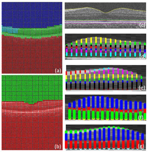
Optical coherence tomography (OCT) is a powerful and noninvasive method for retinal imaging. In this paper, we introduce a fast segmentation method based on a new variant of spectral graph theory named diffusion maps. The research is performed on spectral domain (SD) OCT images depicting macular and optic nerve head appearance. The presented approach does not require edge-based image information in localizing most of boundaries and relies on regional image texture. Consequently, the proposed method demonstrates robustness in situations of low image contrast or poor layer-to-layer image gradients. Diffusion mapping applied to 2D and 3D OCT datasets is composed of two steps, one for partitioning the data into important and less important sections, and another one for localization of internal layers. In the first step, the pixels/voxels are grouped in rectangular/cubic sets to form a graph node. The weights of the graph are calculated based on geometric distances between pixels/voxels and differences of their mean intensity. The first diffusion map clusters the data into three parts, the second of which is the area of interest. The other two sections are eliminated from the remaining calculations. In the second step, the remaining area is subjected to another diffusion map assessment and the internal layers are localized based on their textural similarities. The proposed method was tested on 23 datasets from two patient groups (glaucoma and normals). The mean unsigned border positioning errors (mean ± SD) was 8.52 ± 3.13 and 7.56 ± 2.95 μm for the 2D and 3D methods, respectively.

1. Introduction

Optical coherence tomography (OCT) is a powerful imaging modality used to image various aspects of biological tissues, such as structural information, blood flow, elastic parameters, change of polarization state, and molecular content (Huang et al., 1991). OCT uses the principle of low coherence interferometry to generate two- or three-dimensional images of biological samples by obtaining high-resolution cross-sectional back-scattering profiles (Fig. 1left). In contrast to OCT technology development which has been a field of active research since 1991, OCT image segmentation has only been more fully explored during the last decade. Segmentation remains one of the most difficult and at the same time most commonly required steps in OCT image analysis. No typical segmentation method exists that can be expected to work equally well for all tasks (DeBuc, 2011). We may classify the OCT segmentation approaches into five distinct groups according to the image domain subjected to the segmentation algorithm. Methods applicable to (1) A-scan, (2) Intensity based B-scan analysis, (3) active contour approaches (frequently in 2-D), (4) analysis methods utilizing pattern recognition, and (5) segmentation methods using 2D or 3D graphs constructed from the OCT datasets.

Fig. 1.

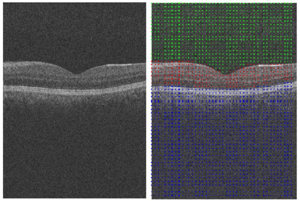
(Left) Example OCT image. (Right) Results of the first diffusion map shown on the right panel, note that the image is partitioned in three regions.

A-Scan methods were introduced by Hee et al. (1995). Since only 2D OCT scanning devices were available at that time, the contribution from 3D context could not be investigated. The mentioned methods also suffered from long computation time (George et al., 2000; Koozekanani et al., 2001) and had limited layer detection accuracy. Additional A-scan approaches have been introduced recently (Fabritius et al., 2009; Koprowski and Wrobel, 2009; Lu et al., 2010). As a good example, Fabritius et al. (2009) incorporated 3D intensity information and segmented the ILM and RPE directly from the OCT data without massive preprocessing in about 17–21 s per 3-D volume with errors smaller than 5 pixels in 99.7% of scans.

Intensity based B-scan analysis methods allowed dealing with 2D noise by incorporating better denoising algorithms during the preprocessing step. However, the dependence of these methods on intensity-based information like boundaries and gradients made them too sensitive to noise, local variations, and threshold value.

Active contour approaches for OCT image segmentation were first proposed by Cabrera Fernández et al. (2004) and modified by Yazdanpanah et al. (2009). Time complexity and exact error reports are not available for the mentioned studies, which make the comparison of these methods with other published methods difficult. Regardless, active contour algorithms surpass the performance of intensity based B-scan approaches, both in resistance to 2D noise and in accuracy.

Pattern recognition based approaches were presented in (Fuller et al., 2007; Mayer et al., 2008) and relied on a multi-resolution hierarchical support vector machine (SVM) or on fuzzy C-means clustering techniques. The former reported to have low ability in detection (6 pixels of line difference and 8% of thickness difference) and a high time complexity (2 min). The latter reported to have better results by 2 pixels of linear difference and 45 s of processing time. The later-introduced methods like graph-based approaches outperformed these techniques in both the accuracy and processing time.

2D or 3D graph-based methods seem so far to be suitable for the task in comparison to the above-mentioned approaches (despite the fact that newly developed A-Scan methods proved to be able to produce accurate and fast results). Their time requirements can be reduced to about 9.74 s per image in 2D graph methods (Chiu et al., 2010) and 45 s per volume for 3D graph methods (Yang et al., 2010). They routinely achieve high accuracy with about 2.8 μm of layer-surface segmentation error. Two dimensional graph-based methods are mainly based on shortest path algorithms (Chiu et al., 2010), whereas three dimensional graph-based methods are usually developed by s–t cut algorithms and take advantage of newly developed 3D imaging systems, which provide better visualization and 3D rendering of the segmentation results (Abràmoff et al., 2009; Lee et al., 2010; Quellec et al., 2010). By design benefitting from contextual information represented in the analysis graph, these methods are robust to noise and do not require advanced noise reduction techniques in the preprocessing steps. While there is no theoretical limit on the number of layers that can be simultaneously segmented by these approaches, up to 10 layers are routinely identified in retinal OCT images.

Table 1 gives an overview of the mentioned approaches and compares the OCT systems, preprocessing methods, error ranges and computation times.

Table 1.

A brief look at different approaches in OCT segmentation. It should be noticed that the number as reported cannot be used for direct comparison of the relative performances, since different settings are utilized in each method.

Segmentation approach	Papers	OCT systems	Preprocessing method	Error range	Computation time
A-scan	Hee et al. (1995), Huang et al. (1991), George et al. (2000), Koozekanani et al. (2001), Gregori and Knighton (2004), Herzog et al. (2004), Shahidi et al. (2005), Ishikawa et al. (2005), Srinivasan et al. (2008), Fabritius et al. (2009), Koprowski and Wrobel (2009), Lu et al. (2010), and Mayer et al. (2010)	TD-OCT (Humphrey 2000, Stratus, OCT 3 Carl- Zeiss Meditec)/SD OCT (Cirrus HD- OCT)	Low-pass filtering, 2D linear smoothing, median filter, non- linear anisotropic filter, Intensity signal based thresholding segmentation	20–36 lm and around 5 pixels in recent papers	Not reported in older cases, but in recent ones like Fabritius et al. (2009), required about 17–21 s for each boundary using a PC With 2.4 GHz CPU, 2.93 GB RAM
Intensity based B-scan analysis	Boyer et al. (2006), Baroni et al. (2007), Tan et al. (2008), Bagci et al. (2008), and Kajić et al. (2010)	TD OCT (OCT 3000 Zees-Humphrey, OCT 2 Carl-Zeiss Meditec, Stratus)/ SDOCT (RTVue100 OCT, Optovue, Freemont, CA)	2D median filter, Gaussian smoothing filtering, bilateral filter	4.2–5 μm	9 s For each image on a Pentium, 1.8 GHz processor with1 GB of RAM
Active contours	Cabrera Fernández et al. (2004), Mishra et al. (2009), Yazdanpanah et al. (2009), and Mujat et al. (2005)	TD OCT (Stratus OCT)/ experimental HR OCT (high speed) / experimental FD- OCT	Nonlinear anisotropic diffusion filter, adaptive vector-valued kernel function	Around 10 μm	5–84 s for each image using Pentium 4 CPU, 2.26 GHz
Artificial intelligence	Fuller et al. (2007) and Mayer et al. (2008)	Experimental 3D OCT, SD OCT (Spectralis)	SVM approach, 2D mean filter, directional filtering	Around 18 μm	45–120 s on a 2 GHz Pentium IV on a computer with 3 GB of RAM (dual processor 3 GHz Intel Xeon)
2D or 3D graphs	Garvin et al. (2008), Abràmoff et al. (2009), Lee et al. (2010), Yang et al. (2010), Quellec et al. (2010), Chiu et al. (2012), and Chiu et al. (2010)	TD OCT (Stratus OCT)/SD OCT (Cirrus–OCT Topcon 3D OCT- 1000)	2D spectral reducing anisotropic diffusion filter, median filtering, wavelets	2.8–6.1 μm	In 2D approach, 9.74 s per image (64-bit OS, Intel Core2 Duo CPU at 2.53 GHz, and 4 GB RAM). In 3D approach, 45–300 s for each 3D volume using a Windows XP workstation with a 3.2 GHz Intel Xeon CPU/on a PC with Microsoft Windows XP Professional x64 edition, Intel core 2 Duo CPU at 3.00 GHz, 4 GBRAM, 16 s in fast segmentation mode

In this paper, we focus on novel spectral-geometric methods for graph based image segmentation and explore a two-step diffusion map approach for the segmentation of OCT images. Many different spectral approaches on graphs have already been introduced, which can be applied on gray-level images. In order to have a comparison between diffusion maps and such approaches, we may consider the theoretical background of “normalized cuts” (N-Cuts) (Shi and Malik, 2000). N-Cuts method is originally based on classification to two subclasses according to the sign on the values in second smallest eigen-vector. Diffusion maps allow the number of clusters to be automatically determined by analyzing the spectra of the image embedding and they are able to steer the diffusion time and granularity of the graph. Another superiority of diffusion maps over N-Cuts is the possibility of coarse graining in diffusion maps which makes the results stable in different runs.

Our research demonstrates the ability of diffusion maps to segment gray-level images. To the best of our knowledge, this is the first report of such a method for OCT segmentation. “Diffusion maps” have a wide range of application in medical image segmentation (Andersson, 2008; Neji et al., 2009; Shen and Meyer, 2006; Wassermann et al., 2007). However, it seems that investigators so-far employed images from high dimensionality modalities like Diffusion MRI, fMRI and/or spectral microscopic images. The OCT images analyzed here are simple single-channel gray level image datasets. In this context, two important points may be noted: A: Every algorithm capable of dealing with high dimensionality is able to handle low dimensional datasets. B: In order to reduce the effects of unavoidable noise in OCT images and to get rid of the complicated and time-consuming noise reduction in the preprocessing step, more than one pixel (or voxel) can be grouped to represent a single node of our graph and textural features (statistics, co-occurrence matrix, run-length matrix) can be derived from each node to measure similarity between nodes. Such features can increase the dimensionality of the dataset and give advantage of dimensionality reduction properties of the diffusion maps. (In this paper we only use geometrical information and the mean intensity of each node and other features should be tested in future works).

2. Methods

In this section we explain the relationship between the theory and performance of the proposed method in separate subsections. We provide an overview of coarse grained diffusion maps in Section 2.1. A concise definition of data points and graph in 2D/3D data is presented in Section 2.2. Section 2.3 is devoted to definition of affinity/distance and kernel in 2D/3D datasets. In order to figure out the total procedure proposed in this paper, a block diagram of the approach is demonstrated in Section 2.4 and the cascade style approach during the segmentation of 2D/3D data is elaborated in Sections 2.4.1 and 2.4.2.

This research is performed on spectral domain (SD) OCT images depicting macular and optic nerve head appearance. The overall algorithm for both appearances is similar and small modifications should be applied on the algorithm for each modality. A list of needed changes for each modality is explained in Section 2.5. A detailed description of parameter selection is set apart in Section 2.6 to clarify the effect of parameters in this research. The proposed algorithm for computation of the number of clusters is presented in the last Section 2.7, and a step by step algorithm for automatic computation of the number of clusters is developed in Section 2.7.1.

2.1. Overview of coarse grained diffusion maps

An overview of coarse grained diffusion maps is presented in this section. We start with introducing diffusion maps and coarse graining algorithms and then a detailed discussion on the implementation of diffusion maps is set up to pinpoint the steps of this algorithm.

2.1.1. Diffusion maps

Diffusion maps (Coifman and Lafon, 2006) form a spectral embed ding of a set X of n nodes, for which local geometries are defined by a kernel k:X × X → R. The kernel k must satisfy k(x, y) ≥ 0, and k(x, y) = k(y, x). One may consider the kernel as an affinity between nodes which results in a graph (an edge between x and y carries the weight k(x, y)). The graph can also be defined as a reversible Markov chain by normalized graph Laplacian construction. We define

$$s\left(x\right)=\sum _{y}k(x,y)$$ (1)

and

$$p_1(x,y)=\frac{k(x,y)}{s\left(x\right)}$$ (2)

This new kernel is not symmetric, but it satisfies the requirements of being the probability of the transition from node x to node y in one time step, or a transition kernel of a Markov chain:

$$\forall x,\sum _y{p}_1(x,y)=1$$ (3)

P is the Markov matrix whose elements are p₁(x, y) and the elements of its powers P^τ are the probability of the transition from node x to node y in τ time steps. The geometry defined by P can be mapped to Euclidean geometry according to eigen-value decomposition of P.

Such a decomposition results in a sequence of eigen-values λ₁, λ₂, … and corresponding eigen-functions ψ₁, ψ₂, … that fulfill Pψ_i = λ_iψ_i. The diffusion map after τ time steps Ψ_τ:X → R^ω embeds each node i = 1, …, n in the Markov chain into an ω-dimensional Euclidean space. Any kind of clustering like κ-means may be done in this new space

$$i\to {\Psi }_{\tau }\left(i\right)=\left(\begin{array}{c}\hfill {\lambda }_1^{\tau }{\psi }_1\left(i\right)\hfill \\ \hfill {\lambda }_2^{\tau }{\psi }_2\left(i\right)\hfill \\ \hfill ⋮\hfill \\ \hfill {\lambda }_{\omega }^{\tau }{\psi }_{\omega }\left(i\right)\hfill \end{array}\right)$$ (4)

It is usually proposed to use a Gaussian kernel for the kernel k(.,.), i.e. $k(x,y)=\exp \left(-\frac{d^2(x,y)}{2{\sigma }^2}\right)$, where d is a distance over the set X and σ is a scale factor.

2.1.2. Coarse graining

This step identifies the best possible clustering of the data points. As described above, P^τ has elements which show the probability of the transition from node x to node y in τ time steps (the time τ of the diffusion plays the role of a scale parameter in the analysis and we chose τ = 1 to work in the original scale). This parameter can be useful in upcoming research relating the diffusion map (Fourier on graphs) to diffusion wavelet (time–frequency approach on graphs), where the scaled versions of the graphs are needed (Kafieh and Rabbani, 2013). The consequences of choosing other values than 1 for scale parameter τ is further elaborated in Section 2.6.

If we do not apply coarse graining algorithm, the random start of k-means algorithm will yield different segmentation results, some of which may be due to the spatial location of first start seeds; However, with coarse graining, a kind of iterative approach will be utilized which ensures the selection of best clustering result in each run and accordingly the same result in multiple runs. Below is a summary of coarse-graining approach in diffusion maps, proposed by Lafon and Lee (2006). According to this approach, if the graph is connected, we have:

$$\underset{\tau \to +\infty }{\lim }{p}^{\tau }(x,y)={\Phi }_0\left(y\right),$$ (5)

A unique stationary distribution (Φ₀), proportional to the density of x in the graph can be defined by:

$${\Phi }_0\left(x\right)=\frac{d\left(x\right)}{\sum _{z}d\left(z\right)}$$ (6)

Similar to Nadler et al. (2006a,b) and Lafon and Lee (2006) defined the “diffusion distance” D_τ between x and y as the weighted L² distance

$$D_{\tau }^2(x,z)={\Vert p^{\tau }(x,.)-p^{\tau }(z,.)\Vert }_{1∕{\Phi }_0}^2=\sum _{y\in \Omega }\frac{{\left(p^{\tau }\right(x,y)-p^{\tau }(z,y\left)\right)}^2}{{\Phi }_0\left(y\right)}$$ (7)

where the “weight” $\frac{1}{{\Phi }_0\left(y\right)}$ gives more penalty to domains with low density than those of high density. Taking into account Eqs. (4) and (7), the diffusion distance can be approximated to relative precision δ using the first q(τ) non-trivial eigen-vectors and eigen-values according to:

$$D_{\tau }^2(x,z)\simeq \sum _{j=1}^{q\left(\tau \right)}{\lambda }^{2\tau }{\left({\psi }_j\right(x)-{\psi }_j(z\left)\right)}^2={\Vert {\Psi }_{\tau }\left(x\right)-{\Psi }_{\tau }\left(z\right)\Vert }^2$$ (8)

where q(τ) is the largest index j such that ∣λ_j∣^τ > δ∣λ₁∣^τ.

In order to retain the connectivity of the graph points, resembling the intrinsic geometry, the coarse-grained graph $\tilde{G}$ with similar spectral properties can be constructed by grouping the nodes of the original graph. The weights between new nodes can also be obtained by averaging the weights between these new node sets. The important point is choosing the groups of nodes in a way that the quantization distortion is minimized.

First, a random partition {S_i}_1≤i≤k may be considered and the members of each set S_i are aggregated to form a node in a new graph $\left(\tilde{G}\right)$ with k nodes. The weights of this graph can be calculated as:

$$\tilde{\omega }(S_i,S_j)=\sum _{x\in S_i}\sum _{y\in S_j}{\Phi }_0\left(x\right)p^{\tau }(x,y),$$ (9)

where the sum accumulates all the transition probabilities between points x ∊ S_i and y ∊ S_j (Fig. 2).

Fig. 2.

Example of the coarse-graining of a graph (Lafon and Lee, 2006).

By setting:

$${\tilde{\varphi }}_0\left(S_i\right)=\sum _{x\in S_i}{\varphi }_0\left(x\right)$$ (10)

the new graph is symmetric. A reversible Markov chain can be defined on this graph:

$$\tilde{p}(S_i,S_j)=\frac{\tilde{\omega }(S_i,S_j)}{\sum _k\tilde{\omega }(S_i,S_j)}=\sum _{x\in S_i}\sum _{y\in S_j}\frac{{\varphi }_0\left(x\right)}{{\tilde{\varphi }}_0\left(S_i\right)}{p}_{\tau }(x,y)$$ (11)

where $\tilde{p}(.,.)$ are the elements of matrix $\tilde{P}$, a k × k transition matrix of the newly developed coarse-grained matrix. The above definition can be similarly defined for 0 ≤ l ≤ n − 1

$${\tilde{\varphi }}_l\left(S_i\right)=\sum _{x\in S_i}{\varphi }_l\left(x\right)$$ (12)

According to duality condition, we may also define:

$$\tilde{\psi }\left(S_i\right)=\frac{{\tilde{\varphi }}_l\left(S_i\right)}{{\tilde{\varphi }}_0\left(S_i\right)}$$ (13)

The above vectors are expected to approximate the right and left eigen-vectors of $\tilde{P}$ and the choice of the partition S_i is the most important factor in finding the best approximation.

To have a measure of such an approximation, distortion in diffusion space should be evaluated. Distortion minimization can be written as a kernel k-means defined in (Lafon and Lee, 2006).

The steps of such an algorithm may be summarized as:

1. Step 0: initialize the partition ${\left\{S_i^{\left(0\right)}\right\}}_{1\le i\le k}$ at random in the diffusion space,

2. For p > 0, update the partition according to

   $$S_i^{\left(p\right)}=\left\{x\mathit{such}\mathit{that}i=\stackrel{\mathit{argmin}}{j}{\Vert {\Psi }_{\mathrm{t}}\left(x\right)-c\left(S_j^{(p-1)}\right)\Vert }^2\right\}$$ (14)

   where 1 ≤ i ≤ k, and $\left(S_j^{(p-1)}\right)$ is the geometric centroid of $S_j^{(p-1)}$.

3. Repeat point 2 until convergence.

2.1.3. Detailed discussion on implementation of diffusion maps

In this section we discuss the important details of this process in six distinct steps.

The first step in diffusion maps is the construction of input data points (the nodes of the graph) with desired dimension. For instance, in the case of clustering a point distribution, x and y coordinates of points represent the 2-dimensional input data; however, in gray level images, the intensity of points should be considered as the third dimension. There is no doubt that dimensionality can be increased in color images or images with particular patterns. Details describing the selection of such features in a graph based method like N-Cuts can be found in (Shi and Malik, 2000). The important point in selection of data points is that it is not necessary to assign one pixel to one node; instead, we may aggregate a group of pixels/voxels together to form a node which may also be helpful in noise management. Details of selecting proper groups of pixels are presented in Section 2.2.

The second step is construction of distance functions (geometric and feature distances). A distance function is defined by matrices with a size of N × N, where N is the number of input points (nodes of the graph). To form the geometric distance, each element of the matrix is calculated as the Euclidean distance ∥X_(i) − X_(j)∥₂ (or any other distance measure like Mahalanobis, Manhattan, etc.) of points; Furthermore, to construct the feature distance, the Euclidean distance of features ∥F_(i) − F_(j)∥₂ is used. The range of each distance matrix is also calculated to show how wide is the distribution of the data set and to estimate the value of the scale factor (σ). Namely, if the distance matrix ∥F_(i) − F_(j)∥₂(or ∥X_(i) − X_(j)∥₂) range from one point to another, the scale factor σ_feature (or σ_geo is recommended to be 0.15 times this range (detailed discussion on the selection of “0.15” is placed in Section 2.6).

The third step is construction of the kernel (weights of the graph). This kernel can be defined as:

$$k(i,j)=\exp \left(-\frac{{\Vert F_{\left(i\right)}-F_j\Vert }_2^2}{2{\sigma }_{\mathit{feature}}^2}\right)\cdot \{\begin{array}{cc}\exp \left(-\frac{{\Vert X_{\left(i\right)}-X_{\left(j\right)}\Vert }_2^2}{2{\sigma }_{\mathit{geo}}^2}\right)\hfill & \text{if}{\Vert X_{\left(i\right)}-X_{\left(j\right)}\Vert }_2<r\hfill \\ 0\hfill & \mathit{otherwise}.\hfill \end{array}\phantom{\}}$$ (15)

where r determines the radius of the neighborhood that suppresses the weight of non-neighborhood nodes and consequently makes a sparse matrix. The weight matrix should also be normalized:

$$p=D^{-1}k,$$ (16)

where D is the diagonal matrix consisting of the row-sums of k. In this step, a threshold (5 × 10⁻⁶ in our case) can be selected to turn the low values to zero and make a more consistent sparse matrix named symmetric graph Laplacian or Markov matrix.

The fourth step is calculating the eigen-functions of the symmetric matrix. We use the LAPACK (Shi and Malik, 2000) routine for singular value decomposition and obtain the normalized right and left eigen-vectors of the Markov matrix. The normalization can be simply achieved with dividing the eigen-vectors to their first value. The right eigen-vectors are rescaled with eigen-values to calculate the diffusion coordinates in Eq. (4).

The fifth step is applying the k-means clustering on diffusion coordinates and iterating the algorithm for many times to select the clustering result for distortion minimization with coarse graining.

The sixth step is recovering the input data points (nodes) corresponding to each of the clustered diffusion coordinates and replacing the graph partitioning with an image segmentation task.

2.2. Definition of data points and graph

2.2.1. Data points for 2D data

In order to apply the diffusion maps to OCT images, we should first define the graph nodes on the image. The 2D data, on which description we apply the algorithms, have a size of 200 × 1024 and 512 × 650 pixels in our two evaluations. A complete of the datasets is given in Sections 3.1 and 3.2.

In order to reduce the noise in OCT images and to get rid of the complicated and time consuming noise reduction in a preprocessing step (like anisotropic diffusion proposed in many papers in Table 1), we may join more than one pixel (or voxel) as the nodes of our graph and select textural features from each node to measure the similarity between the nodes. A vector is constructed containing the selected features of each node such as mean value (more sophisticated textural features are optional and not part of our implementation). Euclidean (L2) norm was then used. Selection of a group of pixels in order to represent each node of the graph, named sparse graph representation, may be done in many different ways. One of the easiest choices may be to define a square or rectangle of a pre-defined size and divide the whole image into non-overlapping or overlapping windows of the selected size. It should be noted that such a selection may significantly reduce the resolution, particularly on edges which may be located inside of these windows.

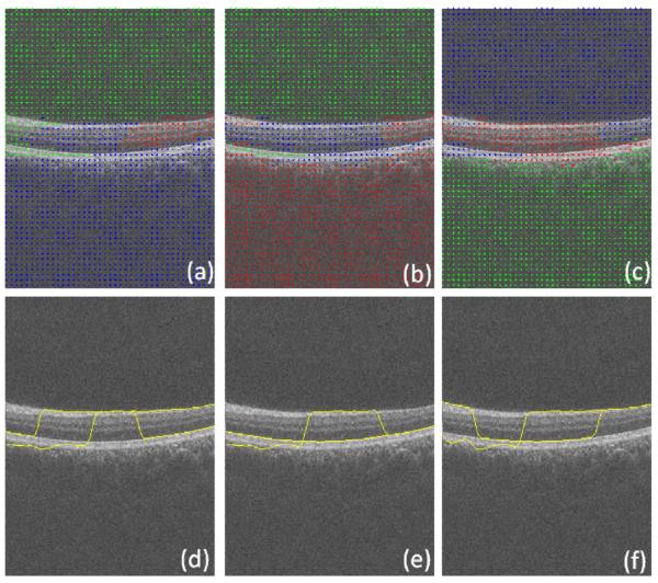
Another way to select multiple points as each node of the graph is selecting the super-pixels (Mori, 2005; Mori et al., 2004; Ren and Malik, 2003). Super-pixels are perceptually meaningful entities obtained from a low-level grouping process. For example, we can apply the Normalized Cuts algorithm to partition an image into super-pixels, the result of applying which on an OCT image is shown in Fig. 3. As it can be seen in Fig. 3, this method is able to select a group of pixels to represent a node in such a way that each group has the lowest possible amount of edges. This can simply lead to the less reduction of resolution which occurres in the rectangular window method, described above. However, the very high time complexity of the super-pixel method (around 3 min for three steps on each image with a size of 650 × 512 pixels), even using mex files in C++, makes this method undesirable for this application.

Fig. 3.

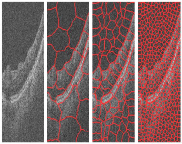
Result of applying super-pixel in three steps to an OCT image.

Another method which may be useful for the selection of groups of pixels as graph nodes is the mean shift algorithm (Paris and Durand, 2007). This method combines the pixels with high degree of similarity and the combined pixels form the nodes of our graph. Fig. 4 shows two examples of such results. However, this method reduces the essential details of OCT images and merges many desired layers which make this procedure inappropriate for our images.

Fig. 4.

Results of applying mean shift to an OCT image. (a, c) Original images. (b, d) Results of mean shift algorithm.

Comparing the proposed strategies (rectangular windowing, super-pixels and mean shift), we found the rectangular method more efficient from the computational and time complexity point of view. The most important drawback of the rectangular windowing algorithm is the decreased resolution which can be improved using a consequent converging step, like active contour searching for the highest gradient to locate the boundaries with an acceptable accuracy.

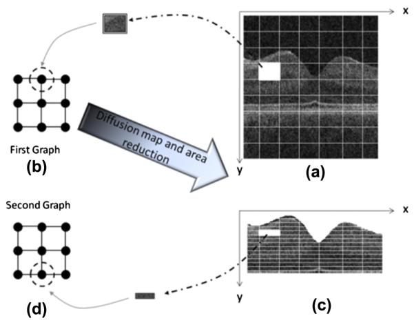
Therefore, we select non-overlapping rectangular windowing in this algorithm. The proposed algorithm consists of two cascade diffusion maps (discussed in more detail in Section 2.4.1), we select 10 × 10 pixel rectangular boxes as graph nodes of the first diffusion map (Fig. 5a) and very thin horizontal rectangles (2 × 20 pixels) are used as graph nodes of the second diffusion map (Fig. 5c).

Fig. 5.

(a) Rectangular windowing on 2D OCT images, (b) allocation of each node to a rectangular portion of 2D OCT images, (c) narrowing the search area to pixels located between the 1st and 7th boundaries and windowing of the new area, and (d) selecting thin horizontal rectangle pixel boxes as the graph nodes.

2.2.2. Data points for 3D data

To implement the diffusion maps on 3D OCT data, each node of the graph is allocated to a cubic portion of the whole 3D data. The 3D data, on which we apply the algorithms, has a size of 200 × 200 × 1024 and 512 × 650 × 128 pixels in our two evaluations. A complete description of datasets is given in Sections 3.1 and 3.2.

Similar to 2D datasets (Section 2.2.1), by accepting the rectangular windowing for our algorithm, we select 10 × 10 × 10 pixel cubes as graph nodes of the first diffusion map (Fig. 6a) and very thin horizontal cubic boxes (15 × 1 pixels) are used as graph nodes of the second diffusion map (Fig. 6c).

Fig. 6.

(a) Cubic windowing on 3D OCTs, (b) allocation of each node to a cubic portion of 3D OCTs, (c) narrowing the search area to pixels located between the 1st and 7th surfaces and windowing of the new area, and (d) selecting thin horizontal cubic pixel boxes as the graph nodes.

2.3. Definition of affinity/distance and kernel

2.3.1. Kernel for 2D data

The proposed algorithm consists of two cascade diffusion maps (discussed in more detail in Section 2.4.1). For each diffusion map, we select graph nodes by rectangular windowing (described in Section 2.2.1 and shown in Fig. 5a and c) and the kernel is defined as:

$$k(x,y)=\exp -\left(\left(\frac{d^2(x,y)}{2{\sigma }_{\mathit{geo}}^2}\right)+\left(\frac{d^2\left(g\right(x),g(y\left)\right)}{2{\sigma }_{\mathit{gray}}^2}\right)\right)$$ (17)

where x, y indicate the centroids of the rectangular boxes, g(.) is the mean gray level of each box, d is the Euclidean distance function introduced in the second step of Section 2.1.3, and σ_geo and δ_gray point out the scale factor, calculated as 0.15 times the range of d(x, y) and d(g(x), g(y)), respectively (detailed discussion on the selection of “0.15” is placed in Section 2.6).

2.3.2. Kernel for 3D data

Similar to 2D algorithm, two cascade diffusion maps (discussed in more detail in Section 2.4.1) are used in 3D the implementation. For each diffusion map, we select graph nodes by rectangular windowing (described in Section 2.2.2 and shown in Fig. 19a and c) and the kernel is defined as:

$$k(x,y,z)=\exp \left(-\frac{d^2(x,y,z)}{2{\sigma }_{\mathit{geo}}^2}\right)\cdot \exp \left(-\frac{d^2\left(g\right(x),g(y),g(z\left)\right)}{2{\sigma }_{\mathit{gray}}^2}\right)$$ (18)

where x, y, z indicate the centroids of selected cubes, g(.) is the mean gray level of each box, d is the Euclidean distance function introduced in the second step of Section 2.1.3, and σ_geo and σ_gray point out the scale factor, calculated as 0.15 times the range of d(x, y, z) and d(g(x), g(y), g(z)), respectively (detailed discussion on the selection of “0.15” is placed in Section 2.6).

Fig. 19.

Selecting the region of interest and choosing 15 × 1 × 15 regions representing the graph nodes (the result is shown on one sample slice).

2.4. Cascade style approach during segmentation

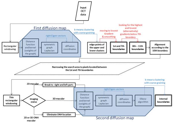
The proposed segmentation algorithm is constructed from a cascade style application of diffusion maps on OCT datasets. We demonstrate the complete process using a block diagram in Fig. 7. Overall the cascade style applies two diffusion maps on each dataset. The first diffusion maps find two boundaries (1st and 7th boundaries in Fig. 7), but the selected boxes as graph nodes (discussed in Section 2.2) have a considerable height and the estimated boundaries need to be refined using gradient information. Another set of boundaries (8th–11th boundaries in Fig. 7), are localized by gradient search starting from the 7th boundary. Finally, the internal boundaries (Fig. 7) are localized using the second diffusion maps and since the selected boxes as the graph nodes of the second diffusion map (discussed in Section 2.2) are determined to be thin, no gradient search is needed for refinement. Sections 2.4.1 and 2.4.2 describe the details of this approach for 2D and 3D data, respectively.

Fig. 7.

Block diagram of the complete process. Blue trapezoids show first and second diffusion maps, boxes with thick border show the results of algorithm (boundaries), and red arrows show gradient-based steps. (For interpretation of the references to colour in this figure legend, the reader is referred to the web version of this article.)

2.4.1. Cascade style for 2D data

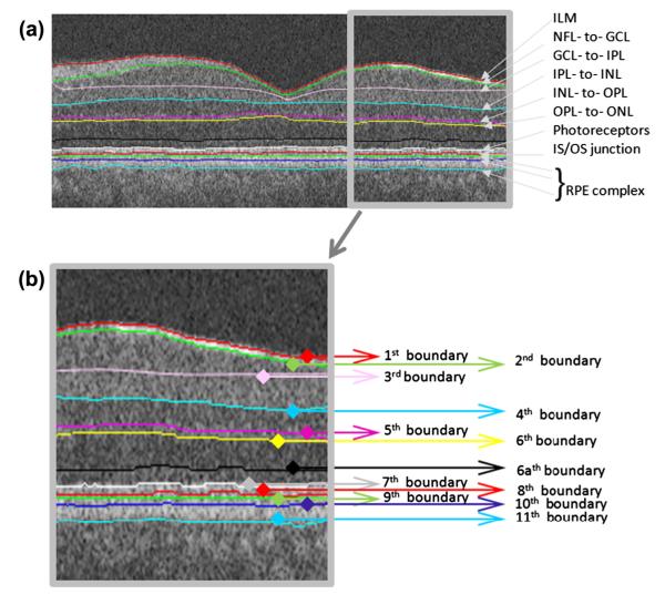
In order to apply the diffusion maps to an OCT image, graph nodes must be associated with the image pixels/voxels. We employ the diffusion map in two sequential steps, the first of which segments six boundaries simultaneously, i.e., the 1st and 7th–11th boundaries. The second step identifies the inner boundaries, i.e., 2nd–6th boundaries and the new boundary (which we call 6a) as described in Fig. 8.

Fig. 8.

Final segmentation on the original image. (a) Definition of retinal surfaces, ILM = internal limiting membrane, NFL = nerve fiber layer, GCL = ganglion cell layer, IPL = inner plexiform layer, INL = inner nuclear layer, OPL = outer plexiform layer, ONL = outer nuclear layer, Photoreceptors, IS = Inner segment of rods and cones, OS = Outer segment of rods and cones, RPE = retinal pigment epithelium. (b) Numbering of retinal surfaces in this paper.

For first diffusion map, we select graph nodes by rectangular windowing of OCT images (described in Section 2.2.1 and shown in Fig. 5a and b) and the kernel is defined based on Section 2.3.1. According to the rules of diffusion maps described in Section 2.1.3, we formed the ω = 3 dimensional Euclidean space:

$$i\to {\Psi }_{\tau }\left(i\right)=\left(\begin{array}{c}\hfill {\lambda }_1^{\tau }{\Psi }_1\left(i\right)\hfill \\ \hfill {\lambda }_1^{\tau }{\Psi }_1\left(i\right)\hfill \\ \hfill {\lambda }_3^{\tau }{\Psi }_3\left(i\right)\hfill \end{array}\right)$$ (19)

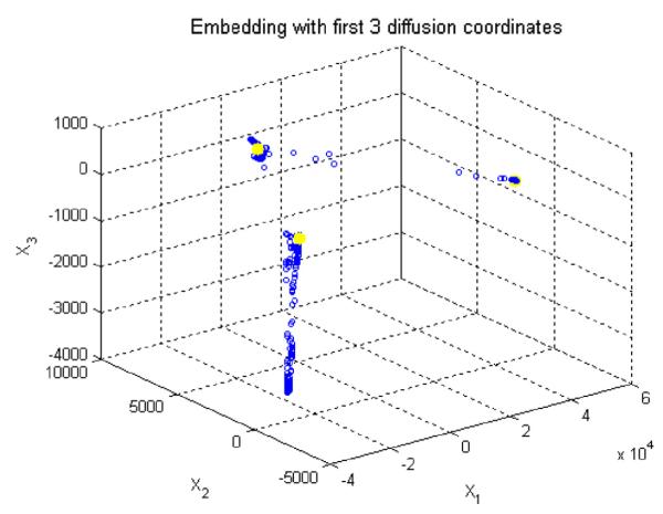
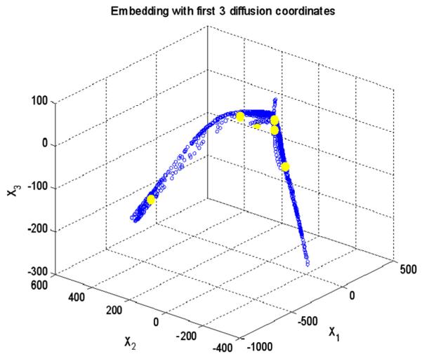
Subsequently, k-means clustering with k = 3 followed by coarse graining is applied to the Euclidean space constructed by eigenfunctions (Figs. 9 right and 9). Since the results of k-means clustering are prone to getting different clustering results in every single run (as a result of randomization of the seed, an intrinsic drawback of this method in the arbitrary selection of start points), the best possible clustering of the data points is achieved by minimizing the quantization distortion using the coarse graining approach. If we do not apply coarse graining algorithm, the random start of k-means algorithm will yield different segmentation results, some of which may be incorrect (merging some layers and differentiating a single layer) due to the spatial location of first start seeds; However, with coarse graining, a kind of iterative approach will be utilized which ensures the selection of best clustering result in each run and accordingly the same result in multiple runs.

Fig. 9.

Applying k means clustering on diffusion coordinates of the first diffusion map, the cluster centroids are shown in yellow and three axes are three most important eigen functions. (For interpretation of the references to colour in this figure legend, the reader is referred to the web version of this article.)

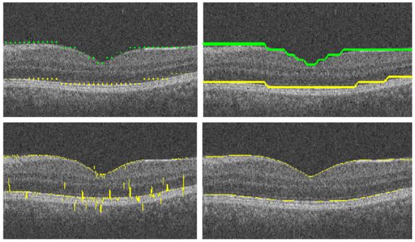
The edge points of the upper and lower clusters are extracted (Fig. 10, top-left) by locating the smallest and the highest values of vertical range in each column. Afterwards, they are connected using a simple linear interpolation (Fig. 10, top-right). It is obvious that the resulting curves are not located exactly on the particular position of edges, due to the size of selected boxes in the first step of diffusion maps. Therefore, the extracted edges are moved to the lowest vertical gradient (Fig. 10, bottom-right and Fig. 11) in a vertical search area of 10 pixels above and 10 pixels below. The results are then enhanced based on applying the following operators on the edges to remove the outliers and to produce a smooth curve: cubic spline smoothing, local regression using weighted linear least squares, and 2nd degree polynomial models (Fig. 10, bottom-right).

Fig. 10.

(Top-left) extracted edge points of the upper and lower clusters. (Top-right) after interpolation. (Bottom-left) after moving to highest gradient. (Bottom-right) after cubic spline smoothing, local regression using weighted linear least squares, and 2nd degree polynomial models.

Fig. 11.

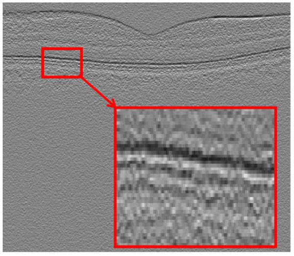
Vertical gradient.

1st and 7th boundaries are obtained in this step and the 8th–11th boundaries are detected by looking for the highest and lowest (alternatively) vertical gradients in a vertical search area of 10 pixels below (Fig. 12, top).

Fig. 12.

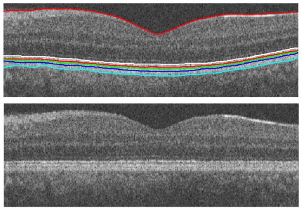
(Top) 1st and 7th–11th boundaries. (Bottom) Linearization.

In most of OCT images, we can see a kind of “geometric distortion” which needs a flattering process (alignment) (Kafieh et al., 2013). It is caused as a result of the relative position of OCT scanner and patient’s pupil, and variation in eye movements. In this algorithm, the geometric distortion of the OCT images is removed according to the 10th boundary to change each column of image in order to produce a linear layer in the place of the 10th border (Fig. 12, bottom).

In the next step, as demonstrated in Fig. 5c, the search area is narrowed to pixels located between the 1st and 7th boundaries and the pixel boxes representing the graph nodes are selected as very thin horizontal rectangles (described in Section 2.2.1 and shown in Fig. 5c and d). This selection is according to the structure of the OCT images after linearization (Fig. 12, bottom). The kernel is defined based on Section 2.3.1 and the k-means clustering is applied with k = 6 (Fig. 13). It should be mentioned that the domain of applying the second diffusion map is decreased to the area located between 1st and 7th boundary and the rest of the image is eliminated. Therefore, the computation time decreases considerably and the segmentation becomes focused on a region of interest.

Fig. 13.

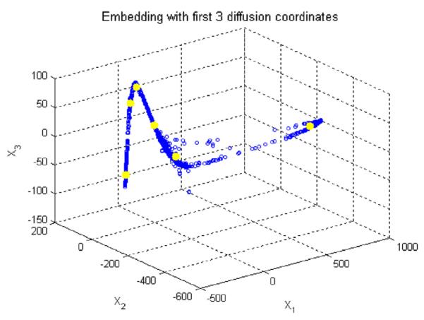
Applying the k means clustering on diffusion coordinates of the second diffusion map, the cluster centroids are shown in yellow and three axes are three most important eigen functions. (For interpretation of the references to colour in this figure legend, the reader is referred to the web version of this article.)

If the OCT image was captured from macula, the area should be divided in two (right and left) parts to increase the accuracy of the method (Fig. 14) since in the case of overall assessment of the images (without breaking to right and left parts), the algorithm couldn’t find proper subgroups. For instance, the first layer in the right and left parts of Fig. 14 has no connections and couldn’t be merged to form a good cluster after employing the diffusion map algorithm (additional insight into splitting the images into right and left parts or any other splitting is elaborated in Section 2.5). In this step, the edge points of clusters were extracted (Fig. 15) and the curves were connected together to form the final segmentation (Figs. 16 and 8a).

Fig. 14.

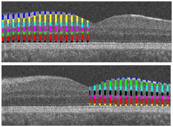
The results of the second diffusion map on the right and left parts of the image.

Fig. 15.

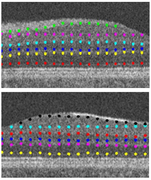
The edge points of clusters.

Fig. 16.

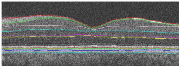
Final segmentation on the aligned image.

One may also use consecutive 2D algorithms applied to each layer of 3D OCT and use the combination of these boundaries to form the 3D surfaces. This idea was tested on our images; however, its time complexity made it impractical. Therefore, a new 3D algorithm was proposed to work on original 3D volumes (Section 2.4.2).

2.4.2. Cascade style for 3D data

Similar to the two-dimensional approach described in Section 2.4.1, we employ the diffusion map in two successive stages (Figs. 6 and 7). In the first stage, six boundaries in 3D (the 1st, and 7^th–11th boundaries, see Fig. 8) are extracted concurrently. The second step is to identify the inner layers in 3D, i.e., the 2nd–6th boundaries and the new boundary (labeled 6a).

For first diffusion map, we select graph nodes by rectangular windowing of OCT datasets (described in Section 2.2.2 and shown in Fig. 6a and b) and the kernel is defined based on Section 2.3.2. A three dimensional Euclidean space is constructed according to Eq. (19) and the k-means clustering with k = 3 followed by coarse graining is applied to the Euclidean space constructed by eigenfunctions (Fig. 17).

Fig. 17.

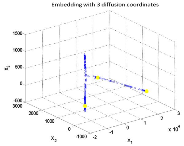
Applying the k means clustering on diffusion coordinates of the first diffusion map in 3D, the cluster centroids are shown in yellow and three axes are three most important eigen functions. (For interpretation of the references to color in this figure legend, the reader is referred to the web version of this article.)

Cubic spline smoothing, local regression using weighted linear least squares, and 2nd degree polynomial models are sequential steps applied to the edge points of the upper and lower clusters in 3D. In order to move the points to the lowest vertical gradient, one may consider the 3D volume as a combination of consecutive 2D slices and search the vertical area in each slice; however, to overcome the time complexity, the gradient search was only applied in selected slices which were located in the borders of the determined cubes with a size of 10 × 10 × 10 (described in Section 2.2.2 and shown in Fig. 6a). The boundaries of remaining slices were then determined using simple interpolation (Fig. 18, top). In the next step, the whole 3D volume was subjected to a 3D drift removing algorithm according to 10th boundary (Fig. 18, bottom).

Fig. 18.

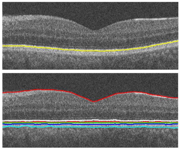
Boundaries (like 1st and 7th) were refined by gradient-based search only in selected slices, which coincided with the borders of the determined cubes. The boundaries in all remaining slices were determined using interpolation. (Top) Border detection using interpolation. (Bottom) Image alignment in 3D (the result is shown on one sample slice).

The following step is eliminating the area located above the 1st boundary and below the 7th boundary (Fig. 19 and Fig. 6c), choosing the graph nodes as described in Section 2.2.2 with a kernel defined in Section 2.3.2, and applying the k-means clustering with k = 6 (Fig. 20). The selected blocks are thin in the y direction to provide the best possible resolution in the detection of internal layers.

Fig. 20.

Applying the k means clustering on diffusion coordinates of the second diffusion map in 3D, the cluster centroids are shown in yellow and three axes are three most important eigen functions. (For interpretation of the references to color in this figure legend, the reader is referred to the web version of this article.)

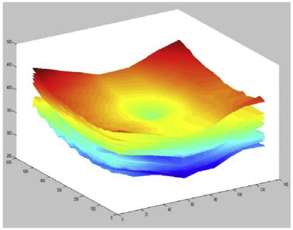
In the final step, 3D boundaries form the final segmentation can be shown (Figs. 21 and 22).

Fig. 21.

Final segmentation on 3D OCT.

Fig. 22.

(Up-left) Surface 1. (Up-right) 1stand 7th surfaces. (Bottom-left) Surfaces 8–11. (Bottom-right) Surfaces 2–6. All results have been produced after alignment based on the hyper-reflective complex (HRC) layer.

2.5. Needed changes for each modality

This research is performed on spectral domain (SD) OCT images depicting macular and optic nerve head appearance. The overall algorithm for both appearances is similar and small modifications should be applied on the algorithm for each modality.

The general algorithm is the same for each modality until thin rectangular/cubic windowing. A decision block in Fig. 7 shows the point in which the modality should be considered. A list of needed changes for each modality is explained through four following states:

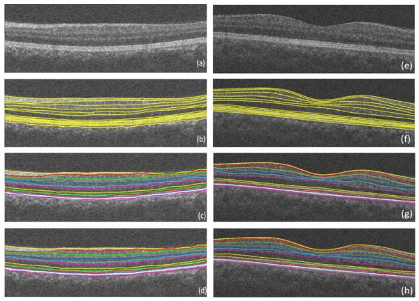
State 1: For the 2D approach on macular images, we separate the central one third of the image after alignment and look for a possible minimum of the first boundary. If the minimum is located in the middle (valley-shaped slices), we select the minimum pixel as the point from which the image should be split (Fig. 14). Otherwise, the minimum of the middle third is on one of the two remaining thirds, it shows a gradual change of the boundary (e.g., Fig. 31a) and we do not need such a separation. Since only in valley-shaped slices we encounter the discontinuity for which we are planning the right and left splitting.

Fig. 31.

Two example results on the Isfahan dataset. (a, e) Composite image. (b, f) Composite image with independent standard. (c, g) Composite image with segmented borders using the 2D approach. (d, h) Composite image with segmented borders using the 3D approach.

This algorithm proposed in State 1 is correct in cases that the fovea (the valley) is centered in the middle third of the image which is valid in our datasets. However, in other cases, the fovea can be localized from a projection image in x–z direction and the algorithm can then be modified to find the breaking point, in a similar method.

State 2: For the 3D approach on macular images, no splitting is needed and all of the thin boxes should go through the second diffusion map.

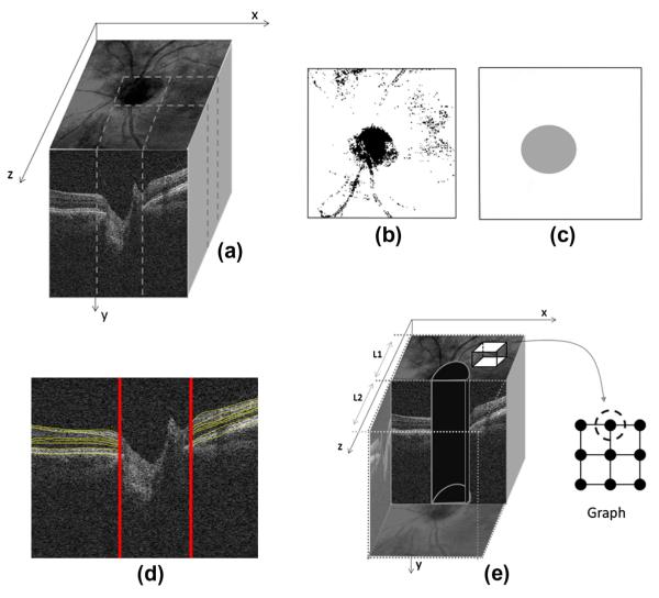
State 3: For the 2D ONH approach, an estimate of the ONH location can be obtained when making a projection image (mean intensity along the y-axis) from a number of slices (Fig. 23a–c). According to the position of the ONH, the nerve head can be omitted from the x–y images and the segmentation is performed on two-sided regions (Fig. 23d). For the alignment purposes, the curves are interpolated in the middle area and the images are aligned according to such interpolated curves.

Fig. 23.

Segmentation of images of the optic nerve head. (a) 3D data. (b) Projection image in x–z direction. (c) ONH mask made according to the projected image. (d) 2D segmentation of ONH images neglecting nerve canal area. (e) Construction of 3D graph while eliminating the central cylindrical volume.

State 4: For the 3D ONH approach, the ONH location can be estimated in the same way as described above. When constructing the graph, the nodes located within a cylinder with an elliptical horizontal cut can be disregarded (Fig. 23e). After computing the first diffusion map, the produced surfaces are non-existent in the middle part and can be interpolated for alignment purposes. The same approach on graph nodes applies to other surfaces resulting from the second diffusion map but no interpolation of the neural canal region is needed (as mentioned in Section 3.1).

2.6. Parameter selection

As described in Section 2.1.1, time of the diffusion plays the role of a scale parameter in the analysis and using higher powers of the kernel (τ > 1) is similar to applying dilation on our graph or calculating the τ-step connections between the nodes. We found that meaningful segmentation results when using single-step connections (τ = 1), while other values of τ resulted in dispersed clusters and undesired divisions. Fig. 24 shows three samples of applying multi-step connections on our first diffusion map.

Fig. 24.

Three samples of applying multi-step connections on our first diffusion map. (a–c) Clusters for τ = 2, 3, 4, respectively. (d–f) Estimated 1st and 7th boundaries after gradient search.

Another parameter, the selection of which should be discussed, is the scale factor (σ). As mentioned in Section 2.1.3, the range of each distance matrix should be found and the scale factors are recommended to be calculated as 0.15 times this range. The choice of the parameter σ is important for the computation of the weights and is a data-dependent parameter (Bah, 2008). Small values of σ will yield almost-zero entries for k(x, y), while large values will lead to close-to-one values (desirable values lie between these two extremes). Based on this idea, Singer (2007) proposed a scheme that was adopted in this work as follows:

1. Construct a sizeable σ-dependent weight matrix k = k(σ) for several values of σ.

2. Compute L(σ = ∑_x ∑_y k_xy(σ).

3. Plot L(σ) using a logarithmic plot. This plot will have two asymptotes when σ → 0 and σ → ∞.

4. Choose σ, for which the logarithmic plot of L(σ) appears linear.

We employed the above algorithm in our application and found that selecting σ equal to 0.15 times the range of distance matrix falls in the linear part of L(σ) and thus there is no need to compute L(σ) separately for each input dataset.

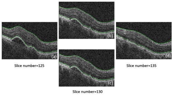
The size of rectangles (or cubes) in the sparse representation of the graphs is an important parameter of the approach. As described in Sections 3.2 and 4, in the 2D approach, the rectangle sizes of the first and second diffusion maps were set to 10 × 10 and 2 × 20, respectively. In the 3D approach, the size of cubes for the first diffusion map were selected as 10 × 10 × 10 and the size of narrow prisms for the second diffusion map was set as 15 × 1 × 15. As discussed above, the second diffusion map is applied on an aligned version of data, where we expect thin and smoothly spread surfaces for different layers. This can be a convincing reason for selecting thin rectangles (or prisms) in this step. In cases with retinal layer pathologies (which were not considered in this work), the surfaces may not be smooth and consequently, such thin rectangles (or cubes) may no longer be appropriate. Fig. 25 shows an example of segmenting a pathologic dataset to demonstrate this problem. Fig. 25a and d shows slices 125 and 135 (10 slice interval), located on the borders of the 3D cubes where the algorithm adjusts the 1st and 7th boundaries with a gradient search. The 130th slice (located inside the cube) does not undergo the gradient search and the 1st and 7th boundaries are found using an interpolation on two sided slices numbered 125 and 135. Fig. 25b shows a result of such interpolation which lacks accuracy. As a solution, one may perform the gradient search on every slice (which requires around six times longer processing time than the previous method) to obtain an acceptable result like that shown in Fig. 25c.

Fig. 25.

Example of applying our approach to pathologic data. (a) Slice number 125, curves obtained by individual gradient search. (b) Slice number 130, interpolated curves. (c) Slice number 130, curves obtained by individual gradient search. (d) Slice number 135, curves obtained by individual gradient search.

Therefore, it seems better to select a smaller number of pixels (or voxels) to construct the nodes. However, this assumption is not totally applicable since if (as an extreme) we select one pixel (or voxel) as a graph node, we lose the important advantage of noise cancellation obtained by the employed simple averaging of pixels. Therefore, the number of allocated pixels (or voxels) per node should be a tradeoff between the desired accuracy and needed noise management in the proposed method.

2.7. Computation of the number of clusters

The algorithm can be evaluated in two modes. One is the automatic mode in which the program identifies the number of layers dynamically and the reported results in this paper are in calculated in this mode. We can also use the algorithm a “user-interface” mode, through which the user can define the number of layers, in advance. Accurate selection of the number of clusters in k-means clustering is important and can be done in at least two ways. The first method is described in (Nadler et al., 2006a, 2006b) and is based on detection of an “elbow” in the eigen-value plots. Briefly, if the slope of the eigen-value plot changes noticeably at the eigen-vector λ_i, the number of clusters should be i + 1. The second way is based on the re-ordering of the rows and columns in the affinity matrix following the second eigen-vector, as proved in (Nadler et al., 2006a, 2006b), which shows the block structure of the matrix as squared blocks along the main diagonal. The number of clusters corresponds to the number of blocks.

The “elbow” algorithm in the first step of diffusion maps on 2D OCT data yields k = 3 as the correct number of clusters (and was used in our algorithms). Fig. 26a shows the eigen-value plot and the plot of $\frac{\lambda }{\lambda -1}$. We may similarly find that k = 6 is, in most of cases, the best cluster number for the second step of the diffusion map algorithm for 2D OCT data (Fig. 26b).

Fig. 26.

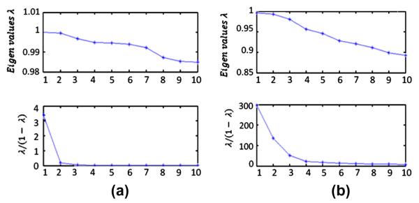
(a) Eigen-value plot in the first step of diffusion maps on 2D OCT data. (b) Eigen-value plot in the second step of diffusion maps on 2D OCT data.

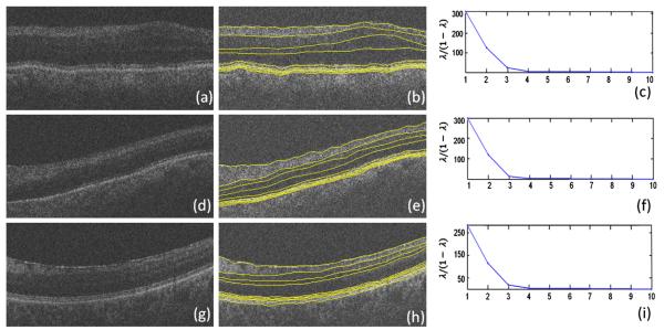
An influential outcome of this method is its ability to determine the proper number of layers in an OCT image, which may vary due to different retinal disorders in the patient, or even as a consequence of using different OCT imaging systems. Fig. 27 shows how our method can be applied to patient data with merged or missing layers due to disease or the limitations of the imaging system. The reported approach is capable of determining the desired number of clusters, a problem that could only be solved manually in the previously reported methods.

Fig. 27.

Application of the proposed method on merged retinal layers (due to pathological appearance or imaging imperfections). (a) Second layer is merged with third layer, and fifth layer is merged with sixth layer, boundary 6a is not visible. (d) Second layer is merged with third layer, and fourth layer is merged with fifth layer, boundary 6a is not visible. (g) Second, third, and fourth layers are merged, boundary 6a is not visible. (b, e, h) Our segmentation method automatically identified the correct number of clusters to segment eight layers (nine surfaces) compared to the usual number of layers. (c, f, i) Eigen-value plots in the second steps of the diffusion map algorithm.

If one selects an incorrect cluster number, two consequences may be expected. If the chosen number is lower than desired, layers will merge; otherwise, if we choose a greater number, over-segmentation will occur. Fig. 28 shows examples of over-segmentation and merging in the first and second diffusion maps. It is obvious that turquoise colors in Fig. 28a, d, and e represent the over-segmented areas and Fig. 28b, f, and g demonstrates region merging.

Fig. 28.

Effects of selecting incorrect number of clusters. (a) First diffusion map. Over segmentation with k = 4. (b) First diffusion map, merging with k = 2. (c) Original image. (d, e) Second diffusion map, over segmentation with k = 8. (f, g) Second diffusion map, merging with k = 4.

We did not encounter the over segmentation problem using elbow algorithm. It should be mentioned that in some cases, very faint boundaries may not be distinguished by elbow algorithm and in order to solve the problem, a step by step algorithm is elaborated in Section 2.7.1, which identifies the merged layers and looks for the missed boundary to compensate the under segmentation problem. It is also important to emphasis that the outer retinal layers (numbered 7–11) are segmented using standard edge gradient consideration, and therefore these layers are not affected by choice of k in the second diffusion maps.

2.7.1. A step by step algorithm for computation of the number of clusters

As discussed above, an influential outcome of this method is its ability to distinguish the proper number of layers in an OCT image. It should be mentioned that in some cases, very faint boundaries may not be distinguished by this method and two strategies may be developed: one is ignoring the missed layers, and the second method is setting a new diffusion map in the area of the missed layers. The second approach is applicable in missing boundaries, the anatomical existence of which are certain. Then, we may choose two boundaries positioned above and below the missed layer and remove the information out of this area (similar to operations performed in Figs. 5 and 6). A new graph and diffusion map can then be employed to find the missed layers (as it is used in Section 3.2 to find the second layer (third boundary) and is demonstrated in Fig. 29).

Fig. 29.

Determining missed boundaries using successive diffusion maps.

Following the “elbow” algorithm, k = 6 was identified as the best cluster number (in general) for the second step of the diffusion map algorithm for our 2D OCT data. The cluster number was correct for the dataset used in Section 3.1, where the ELM/ISL interface was not clearly distinguishable and GCL/IPL interface was recognizable; however, using k = 6 results in an incorrect segmentation in images, in which the ELM boundary exists explicitly while the GCL/IPL interface is very faded (like dataset used in Section 3.2). In such cases, the existence of a clear boundary 6a, forces the algorithm to localize this boundary and miss a less visible boundary located between GCL and IPL. While we may apply k = 7 (manually) and obtain the correct localization of all layers (as demonstrated in Fig. 14), this is not an acceptable solution. Not only does it make our algorithm non-automated in the detection of cluster numbers, but also this incorrect selection occurs in many cases. The solution is shown in Fig. 29. As described above, two boundaries located above and below the known anatomical boundary may be selected in the next step and the diffusion map algorithm can be applied to the region located between them to find the missed edge.

To sum up, the steps for the automatic computation of the number of clusters are as follows:

• Step (1) Run the algorithm using the number of clusters obtained from the “elbow” algorithm.

• Step (2) Calculate the mean vertical distances between the lowest localized boundary to two closest boundaries below and above.

• Step (3)

  1. If the lowest boundary is nearer to the upper boundary than the lower one, we assume that the algorithm operates under normal conditions and that there is no need to take an extra action (similar to datasets used in Section 3.1). Then go to Step 6.
  2. If, however, the lowest boundary is nearer to the lower boundary than the upper one, the existence of a detectable ELM/ISL boundary is assumed. Then go to Step 4.
• Step (4)

  1. If the calculated number of clusters by the algorithm (using the eigenvalue method) is k = 6, normal condition is assumed (with no merged layers due to pathology or imaging artifacts), but a faded GCL/IPL interface exists, then go to Step 5 (similar to datasets used in Section 3.2).
  2. If the calculated number of clusters by the algorithm (using the eigenvalue method) is less than k = 6, an abnormal condition is assumed with merged layers (due to pathological appearance or imaging imperfections, examples of this condition can be found in Fig. 27). Then go to Step 6.
  3. If the calculated number of clusters by the algorithm (using eigenvalue method) is k = 7, a normal condition is assumed (with no merged layers due to pathology or instrument), and the GCL/IPL interface is expected to be clear enough to be distinguished, then go to Step 6.

• Step (5) Run another Diffusion map algorithm with k = 2 in the area located between the second and third boundaries (as shown in Fig. 29) to localize GCL/IPL interface. Then go to Step 6.

• Step (6) Plot the boundaries and stop the algorithm.

The computation time of the proposed algorithms (implemented in MATLAB™ without using the mex files-Math Works, Inc., Natick, MA (MATLAB™ version 7.8-Math Works, 2009) were 12 s for each image using 2D approach and 230 s for each 3D volume using the 3D approach. The time complexity of the combined method (which used an interpolation on 2D results to estimate the 3D segmentation) was 1600 s. A PC with Microsoft Windows XP x32 edition, Intel core 2 Duo CPU at 3.00 GHz, 4 GB RAM was used for the 2D approach and Windows XP x64 edition workstation with a 3.2 GHz Intel Xeon CPU, 32 GB RAM was used for the 3D approach.

3. Experiments and results

The application of diffusion maps to the segmentation of OCT images is presented in 2D and 3D. To evaluate the capability of this method, 23 datasets from two patient groups were analyzed. The first group consisted of 10 OCT images from 10 patients diagnosed with glaucoma (Antony et al., 2010). The independent standard resulted from averaging tracings from two expert observers and performance assessment results are given in Section 3.1. The second group (the Isfahan dataset) was obtained from 13 normal eyes from 13 subjects and the validation was based on averaged tracings by two expert observers (Section 3.2).

The overall topology of the localized retinal layers is correct and according to anatomical structures due to the allocation of thin boxes for each node. We also put a constraint on each segmented boundary to be placed beneath the upper band. Furthermore, the boundaries are required to cover the whole width/surface (in 2D and 3D approach, respectively); otherwise, the missed values are inter/extrapolated.

We use step by step algorithm for the automatic computation of the number of clusters (described in Section 2.7.1) for the reported results which identifies the number of layers dynamically. The first set is evaluated by 3D approach of the algorithm (Section 3.1) and the second set is evaluated by both 2D and 3D approaches (Section 3.2).

3.1. Experimental results on the glaucomatous test set

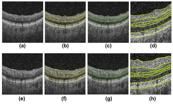
In order to have a comparison with results of Lee et al. (2010) and Antony et al. (2010), we applied our 3D algorithm to a glaucoma OCT dataset (Cirrus, Zeiss Meditec) (Antony et al., 2010). Two example results are shown in Fig. 30. Since the independent standard available for the datasets contained a subset of seven retinal surfaces, only seven surfaces (out of the complete set of detected boundaries) are used for comparison.

Fig. 30.

Two example results obtained on the glaucoma test set. (a, e) Composite image. (b, f) Composite image with computer-segmented borders. (c, g) Composite image showing independent standard. (d, h) Comparison of computer-segmentation (yellow) and independent standard (green). (For interpretation of the references to colour in this figure legend, the reader is referred to the web version of this article.)

The testing set for the validation of the segmentation algorithm consisted of 10 datasets from 10 patients diagnosed with glaucoma. Each dataset had the x, y, z dimensions of 6 × 2 × 6 mm³, 200 × 1024 × 200 voxels sized 30 × 1.95 × 30 μm³ (Fig. 6). The algorithm was tested against the manual tracings of two independent observers on 10 slices selected randomly in each dataset and seven retinal layers.

For validation, the mean signed and unsigned border positioning errors for each border were computed and are presented in Tables 2 and 4 for each boundary, differences were not computed in the neural canal. The evaluation algorithm is modified to test only seven surfaces out of 12 boundaries shown in Fig. 8. To show statistically significant improvement of the proposed method over the algorithms reported in (Lee et al., 2010; Antony et al., 2010), Table 3 shows the obtained p-values.

Table 2.

Summary of mean unsigned border positioning errors (mean ± sd) in micrometers.

Border	Avg. obs. vs. our alg.	Avg. obs. vs. alg. in Lee et al. (2010)	Avg. obs. vs. alg. in Antony et al. (2010)	Obs. 1 vs. obs. 2
1	4.11 ± 1.17	6.73 ± 3.95	4.90 ± 1.54	4.90 ± 1.37
2	8.60 ± 4.11	14.64 ± 4.26	14.43 ± 5.63	12.79 ± 3.36
4	9.19 ± 3.13	11.52 ± 3.42	10.96 ± 4.06	13.74 ± 2.04
5	6.45 ± 2.74	10.50 ± 3.33	10.46 ± 2.79	9.28 ± 3.00
6	9.19 ± 2.75	8.87 ± 2.55	10.73 ± 2.78	7.67 ± 1.69
7	2.35 ± 1.56	3.87 ± 0.80	3.87 ± 1.32	4.69 ± 1.26
11	4.11 ± 0.59	6.72 ± 1.44	7.24 ± 1.74	6.58 ± 1.53
Overall	6.32 ± 2.34	8.98 ± 3.58	8.94 ± 3.76	8.52 ± 3.61

Table 4.

Mean signed border positioning errors (mean ± sd) in micrometers.

Border	Avg. obs. vs. alg.	Avg. obs. vs. Lee et al. (2010)
1	1.56 ± 1.04	2.55 ± 1.19
2	−7.56 ± 4.36	−8.33 ± 7.83
4	7.04 ± 4.13	−9.19 ± 3.67
5	−5.28 ± 2.64	−5.44 ± 4.10
6	−6.84 ± 2.19	−6.63 ± 2.96
7	1.17 ± 0.92	1.54 ± 1.09
11	−1.76 ± 1.49	−1.86 ± 3.01
Overall	−1.69 ± 2.52	−3.91 ± 4.71

Table 3.

Improvement of the proposed method compared with algorithms Lee et al. (2010) and Antony et al. (2010).

Border	p Value our alg. vs. alg. in Lee et al. (2010)	p Value our alg. vs. alg. in Antony et al. (2010)
1	<<0.001	<0.001
2	<<0.001	<<0.001
4	<0.001	<0.001
5	<<0.001	<<0.001
6	0.8022	<0.001
7	<<0.001	<<0.001
11	<<0.001	<<0.001
Overall	<<0.001	<<0.001

Furthermore, the errors of mean layer thicknesses determined as the distances from the first to other surfaces are computed and shown in Table 5.

Table 5.

Mean absolute thickness differences (mean ± sd) in micrometers.

Border	Avg. obs. vs. alg.
1–2	6.1 ± 3.8
1–4	3.7 ± 2.2
1–5	1.9 ± 1.0
1–6	6.3 ± 3.2
1–7	2.0 ± 1.3
1–11	3.8 ± 2.7

3.2. Experimental results on the Isfahantest Set

The proposed method was tested on thirteen 3D macular SDOCT images obtained from eyes without pathologies using Topcon 3D OCT-1000 imaging system in Ophthalmology Dept., Feiz Hospital, Isfahan, Iran. The x, y, z size of the obtained volumes was 512 × 650 × 128 voxels, 7 × 3.125 × 3.125 mm³, voxel size 13.67 × 4.81 × 24.41 μm³ (Fig. 6).

The OCT images were segmented to locate all of the 10 layers (11 surfaces) as given in (Quellec et al., 2010). Furthermore, one extra surface was identified between the 6th and 7th surfaces (Fig. 8). The validation was based on manual tracing by two observers. Our algorithms in their 2D and 3D versions were applied to this set and the mean signed and unsigned border positioning errors were computed for each surface and presented in Tables 6 and 7.Fig. 31 shows the examples of the achieved results.

Table 6.

Mean unsigned border positioning errors on the isfahan dataset (mean ± sd) in micrometers.

Border	Avg. obs. vs. alg. in 2D approach	Avg. obs. vs. alg. in 3D approach	Obs. 1 vs. obs. 2
1	6.88 ± 3.22	7.53 ± 3.21	6.25 ± 3.12
2	12.82 ± 5.56	10.97 ± 5.15	15.94 ± 8.94
3	10.94 ± 4.13	6.79 ± 2.12	10.63 ± 6.19
4	15.03 ± 5.12	12.87 ± 4.95	16.25 ± 9.27
5	10.05 ± 3.74	8.53 ± 2.64	12.82 ± 5.36
6	13.75 ± 3.18	12.82 ± 5.27	12.53 ± 4.89
6a	6.57 ± 2.13	4.97 ± 1.23	7.81 ± 3.76
7	3.44 ± 1.01	4.38 ± 1.37	5.63 ± 2.23
8	4.07 ± 2.08	4.68 ± 1.39	5.61 ± 2.58
9	5.05 ± 1.29	5.32 ± 2.24	8.42 ± 3.95
10	6.25 ± 2.37	5.31 ± 1.36	6.55 ± 3.84
11	6.88 ± 2.42	6.57 ± 2.84	7.19 ± 2.45
Overall	8.52 ± 3.13	7.56 ± 2.95	9.65 ± 4.83

Table 7.

Mean signed border positioning errors (mean ± sd) in micrometers.

Border	Avg. obs. vs. alg. in 2D approach	Avg. obs. vs. alg. in 3D approach	Obs. 1 vs. obs. 2
1	4.85 ± 2.42	5.13 ± 2.96	−5.34 ± 2.31
2	−13.54 ± 5.65	−10.12 ± 4.65	13.16 ± 6.56
3	−13.22 ± 4.38	−10.29 ± 4.38	13.37 ± 6.39
4	−16.23 ± 5.62	−14.50 ± 5.12	13.06 ± 7.24
5	−7.63 ± 4.21	−7.69 ± 3.19	9.84 ± 5.21
6	−11.34 ± 5.34	−8.37 ± 2.18	12.88 ± 6.13
6a	6.62 ± 1.21	−5.12 ± 3.28	−12.28 ± 2.36
7	3.16 ± 1.24	4.84 ± 2.24	−6.06 ± 2.34
8	3.97 ± 2.12	4.91 ± 1.33	5.91 ± 1.54
9	−3.91 ± 1.65	−4.47 ± 1.49	7.09 ± 2.18
10	−4.16 ± 2.37	−4.44 ± 2.27	7.31 ± 1.94
11	−3.60 ± 2.46	−4.28 ± 1.39	8.97 ± 2.94
Overall	−4.61 ± 3.35	−4.53 ± 2.89	5.71 ± 3.98

3.3. Discussion of results

The numerical results of the proposed algorithm on the Glaucomatous test set are presented in Tables 1–5. Tables 2 and 4 summarize the computed border position errors. According to these tables, the border positioning errors between the algorithm and the reference standard were similar to those computed between the observers. For example, the algorithm’s overall unsigned border positioning error was 6.32 ± 2.34 μm, while the overall observer error was 8.52 ± 3.61 μm.

The border positioning errors show improvement over the algorithms reported in (Lee et al., 2010; Antony et al., 2010). For example the algorithm’s overall unsigned border positioning error was 6.32 ± 2.34 μm, while the unsigned error in (Lee et al., 2010; Antony et al., 2010) were 8.98 ± 3.58 μm and 8.94 ± 3.76 μm, respectively.

Since we did not have access to the mean signed errors of (Antony et al., 2010), we can only report the improvement of signed errors over (Lee et al., 2010). For example the algorithm’s overall signed border positioning error was −1.69 ± 2.52 μm, while the mean signed error in (Lee et al., 2010) was −3.91 ± 4.71 μm.

Table 5 summarizes the thickness difference results. We could not make any comparison to other methods since we didn’t have access to their values.

To show the statistically significant improvement of the proposed method over the algorithms reported in (Lee et al., 2010) and (Antony et al., 2010), Table 3 shows the obtained p-values. Except for the comparison of our method to Alg. (Lee et al., 2010) in the 6th boundary, our results show a significant improvement over the mentioned methods. For instance, the algorithm’s overall p-value against (Lee et al., 2010) and (Antony et al., 2010) were both less than 0.001.

Tables 6 and 7 present the numerical result of the proposed algorithm on the Isfahan test set. Our algorithms in their 2D and 3D versions were applied to this set and the mean signed and unsigned border positioning errors were computed for each surface and presented in Tables 6 and 7.

As can be seen in Tables 6 and 7, the 1st and 7th-to-11th boundaries, which are dependent on the gradient search, are better localized in the 2D approach. As discussed in Section 2.4.2, in order to reduce the computational complexity, the gradient search in 3D approach was only applied to selected slices located in the borders of the determined cubes. The boundaries of the remaining slices were then determined using simple interpolation (Fig. 18, top). Therefore, it is expected that the border positioning error in the 3D approach will be greater than for the 2D method in the gradient-based boundaries. However, the localization error of other boundaries (labeled 2–6a) is lower for the 3D approach because of the global character of the 3D method.

4. Conclusion and future work

A novel method for the automatic segmentation of intra-retinal layers in 2D and 3D SD-OCT scans from glaucoma patients and normal controls was presented. The method is based on the application of two sequential diffusion maps, first of which segments the ILM-to-RPE complex and reduces the data to the region between these two layers. The second map then localizes the internal layers between the ILM and the RPE complexes.

The reported approach outperformed several previously published graph-based methods, which suggests an advantage of the employed texture analysis strategy.

Another important advantage of this method is its ability to make a correct decision regarding the number of clusters in k-means clustering, which, as a result, detects the proper number of layers to be segmented. This may be even more useful in cases for which one or more anatomical layers are not visible due to disease or low image quality.

The experiments suggested the robustness of this method across OCT scanners from different manufacturers, e.g. 3D spectral-domain OCT Zeiss Cirrus and Topcon 3D OCT-1000.

The computation time of this method is relatively low when compared with other methods especially considering its MATLAB implementation.

The robustness of the algorithm in presence of blood vessel artifacts is discussed in many papers (Yang et al., 2010; Hood et al., 2008), and some researchers tried to propose a preprocessing algorithm to compensate for the effect of these vessels (Lu et al., 2010). However, the global approach behind the diffusion maps makes it intrinsically insensitive to small artifacts, as illustrated in Fig. 32.

Fig. 32.

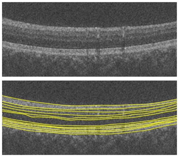
Robustness of the proposed algorithm to blood vessel artifacts.

Another important point to be discussed is the advantage of employing diffusion maps in obtaining an initial rough approximation of the two initially detected boundaries (boundaries 1 and 7). We can compare our method to (Fabritius et al., 2009; Hee et al., 1995; Ishikawa et al., 2005; Koozekanani et al., 2001; Shahidi et al., 2005), which used a similar A-Scan search for finding increases of the noise level to identify ILM and PRE or looked for 1D edges and their maxima in each A-Scan. The most serious problem with these methods was the identification of spurious responses. In contrast, the gradient search in our method is limited to an area around a rough approximation of these boundaries. Therefore, the speed of localization can be improved and the possibility of finding erroneous responses decreases. To have a numerical comparison, we developed the algorithm proposed by Fabritius et al. (2009) (to be one of the fastest methods heretofore) and the computation time of detecting boundaries 1 and 7 using our algorithm and the detection of ILM and PRE using (Fabritius et al., 2009) (on our 3D datasets used in Section 5.2) were comparable for the two methods and both needed around 50 s for completion, demonstrating the similar speed of the two methods.

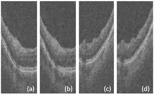
Furthermore, to find the rough approximation, Ghorbel et al. (2011) proposed a k-means clustering on OCT image which did not produce a discriminative segmentation (Fig. 33) and the authors defined a great deal of extra steps to extract the boundaries. Our proposed method, however, performs the clustering in frequency domain and a meaningful segmentation is achieved simply requiring a subsequent gradient search to produce a final segmentation. The time complexity is also low since the image resolution is reduced by employing small regions in the sparse representation.

Fig. 33.

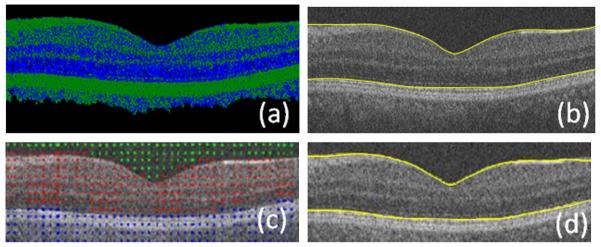
A comparison of clustering in (Ghorbel et al., 2011) and in the proposed method. (a) Clustering result obtained using Ghorbel’s method (Ghorbel et al., 2011). (b) Segmentation resulting from the Ghorbel’s method (Ghorbel et al., 2011). (c) Clustering obtained using the reported method. (d) Segmentation resulting from the proposed method.

In our future work, we will focus on the applications of diffusion wavelets (Coifman and Maggioni, 2006) on OCT images and will investigate their possible ability for noise removal, segmentation and detection of abnormalities of retinal OCT images (Kafieh and Rabbani, 2013).

References

- Abràmoff MD, Lee K, Niemeijer M, Alward WL, Greenlee EC, Garvin MK, Sonka M, Kwon YH. Automated segmentation of the cup and rim from spectral domain OCT of the optic nerve head. Investigative Ophthalmology & Visual Science. 2009;50:5778–5784. doi: 10.1167/iovs.09-3790. [DOI] [PMC free article] [PubMed] [Google Scholar]
- Andersson J. Master Thesis at Dep. Math. Royal Academy of Science. 2008. Diffusion Geometry with Applications to Virus Classification. Trita-mat-2008-11. [Google Scholar]
- Antony BJ, Abràmoff MD, Lee K, Sonkova P, Gupta P, Kwon Y, Niemeijer M, Hu Z, Garvin MK. Automated 3D segmentation of intraretinal layers from optic nerve head optical coherence tomography images, SPIE Medical Imaging. International Society for Optics and Photonics. 2010:76260U–76260U-76212. [Google Scholar]
- Bagci AM, Shahidi M, Ansari R, Blair M, Blair NP, Zelkha R. Thickness profiles of retinal layers by optical coherence tomography image segmentation. American Journal of Ophthalmology. 2008;146:679. doi: 10.1016/j.ajo.2008.06.010. [DOI] [PMC free article] [PubMed] [Google Scholar]
- Bah B. Diffusion Maps: Analysis and Applications. University of Oxford; 2008. [Google Scholar]
- Baroni M, Fortunato P, La Torre A. Towards quantitative analysis of retinal features in optical coherence tomography. Medical Engineering & Physics. 2007;29:432–441. doi: 10.1016/j.medengphy.2006.06.003. [DOI] [PubMed] [Google Scholar]
- Boyer KL, Herzog A, Roberts C. Automatic recovery of the optic nervehead geometry in optical coherence tomography. IEEE Transactions on Medical Imaging. 2006;25:553–570. doi: 10.1109/TMI.2006.871417. [DOI] [PubMed] [Google Scholar]
- Cabrera Fernández D, Villate N, Puliafito C, Rosenfeld P. Comparing total macular volume changes measured by Optical Coherence Tomography with retinal lesion volume estimated by active contours. Investigative Ophthalmology and Visual Science. 2004;45:3072. [Google Scholar]
- Chiu SJ, Izatt JA, O’Connell R, Winter K, Toth CA, Farsiu S. Validated automatic segmentation of AMD pathology including drusen and geographic atrophy in SD-OCT images. Investigative Ophthalmology and Visual Science. 2012;53:53–61. doi: 10.1167/iovs.11-7640. [DOI] [PubMed] [Google Scholar]
- Chiu SJ, Li XT, Nicholas P, Toth CA, Izatt JA, Farsiu S. Automatic segmentation of seven retinal layers in SDOCT images congruent with expert manual segmentation. Optics Express. 2010;18:19413. doi: 10.1364/OE.18.019413. [DOI] [PMC free article] [PubMed] [Google Scholar]
- Coifman RR, Lafon S. Diffusion maps. Applied and Computational Harmonic Analysis. 2006;21:5–30. [Google Scholar]
- Coifman RR, Maggioni M. Diffusion wavelets. Applied and Computational Harmonic Analysis. 2006;21:53–94. [Google Scholar]
- DeBuc DC. A review of algorithms for segmentation of retinal image data using optical coherence tomography. Image Segmentation. 2011;15:54. [Google Scholar]
- Fabritius T, Makita S, Miura M, Myllylä R, Yasuno Y. Automated segmentation of the macula by optical coherence tomography. Optics Express. 2009;17:15659–15669. doi: 10.1364/OE.17.015659. [DOI] [PubMed] [Google Scholar]
- Fuller AR, Zawadzki RJ, Choi S, Wiley DF, Werner JS, Hamann B. Segmentation of three-dimensional retinal image data. IEEE Transactions on Visualization and Computer Graphics. 2007;13:1719–1726. doi: 10.1109/TVCG.2007.70590. [DOI] [PMC free article] [PubMed] [Google Scholar]
- Garvin MK, Abràmoff MD, Kardon R, Russell SR, Wu X, Sonka M. Intraretinal layer segmentation of macular optical coherence tomography images using optimal 3-D graph search. IEEE Transactions on Medical Imaging. 2008;27:1495–1505. doi: 10.1109/TMI.2008.923966. [DOI] [PMC free article] [PubMed] [Google Scholar]
- George A, Dillenseger J, Weber A, Pechereau A. Optical coherence tomography image processing. Investigative Ophthalmology and Visual Science. 2000;41:165–173. [Google Scholar]
- Ghorbel I, Rossant F, Bloch I, Tick S, Paques M. Automated segmentation of macular layers in OCT images and quantitative evaluation of performances. Pattern Recognition. 2011;44:1590–1603. [Google Scholar]
- Gregori G, Knighton R. A robust algorithm for retinal thickness measurements using optical coherence tomography (Stratus OCT) Investigative Ophthalmology and Visual Science. 2004;45:3007. [Google Scholar]
- Hee MR, Izatt JA, Swanson EA, Huang D, Schuman JS, Lin CP, Puliafito CA, Fujimoto JG. Optical coherence tomography of the human retina. Archives of Ophthalmology. 1995;113:325. doi: 10.1001/archopht.1995.01100030081025. [DOI] [PubMed] [Google Scholar]
- Herzog A, Boyer KL, Roberts C. Robust extraction of the optic nerve head in optical coherence tomography. Computer Vision and Mathematical Methods in Medical and Biomedical Image Analysis. 2004:395–407. [Google Scholar]
- Hood DC, Fortune B, Arthur SN, Xing D, Salant JA, Ritch R, Liebmann JM. Blood vessel contributions to retinal nerve fiber layer thickness profiles measured with optical coherence tomography. Journal of Glaucoma. 2008;17:519. doi: 10.1097/IJG.0b013e3181629a02. [DOI] [PMC free article] [PubMed] [Google Scholar]
- Huang D, Swanson EA, Lin CP, Schuman JS, Stinson WG, Chang W, Hee MR, Flotte T, Gregory K, Puliafito CA. Optical coherence tomography. Science. 1991;254:1178–1181. doi: 10.1126/science.1957169. [DOI] [PMC free article] [PubMed] [Google Scholar]
- Ishikawa H, Stein DM, Wollstein G, Beaton S, Fujimoto JG, Schuman JS. Macular segmentation with optical coherence tomography. Investigative Ophthalmology & Visual Science. 2005;46:2012–2017. doi: 10.1167/iovs.04-0335. [DOI] [PMC free article] [PubMed] [Google Scholar]
- Kafieh R, Rabbani H. Combination of Graph Theoretic Grouping and Time-Frequency Analysis for Image Segmentation with an Example for EDI-OCT. Applications of Digital Image Processing XXXVI; San Diego, California, United States. SPIE; 2013. [Google Scholar]
- Kafieh R, Rabbani H, Abramoff MD, Sonka M. Curvature correction of retinal OCTs using graph-based geometry detection. Physics in Medicine and Biology. 2013;58:2925. doi: 10.1088/0031-9155/58/9/2925. [DOI] [PMC free article] [PubMed] [Google Scholar]
- Kajić V, Považay B, Hermann B, Hofer B, Marshall D, Rosin PL, Drexler W. Robust segmentation of intraretinal layers in the normal human fovea using a novel statistical model based on texture and shape analysis. Optics Express. 2010;18:14730–14744. doi: 10.1364/OE.18.014730. [DOI] [PubMed] [Google Scholar]
- Koozekanani D, Boyer K, Roberts C. Retinal thickness measurements from optical coherence tomography using a Markov boundary model. IEEE Transactions on Medical Imaging. 2001;20:900–916. doi: 10.1109/42.952728. [DOI] [PubMed] [Google Scholar]
- Koprowski R, Wrobel Z. Layers recognition in tomographic eye image based on random contour analysis. Computer Recognition Systems. 2009;3:471–478. [Google Scholar]
- Lafon S, Lee AB. Diffusion maps and coarse-graining: a unified framework for dimensionality reduction, graph partitioning, and data set parameterization. IEEE Transactions on Pattern Analysis and Machine Intelligence. 2006;28:1393–1403. doi: 10.1109/TPAMI.2006.184. [DOI] [PubMed] [Google Scholar]
- Lee K, Niemeijer M, Garvin MK, Kwon YH, Sonka M, Abràmoff MD. Segmentation of the optic disc in 3-D OCT scans of the optic nerve head. IEEE Transactions on Medical Imaging. 2010;29:159–168. doi: 10.1109/TMI.2009.2031324. [DOI] [PMC free article] [PubMed] [Google Scholar]
- Lu S, Cheung C.-l., Liu J, Lim JH, Leung C.-s., Wong TY. Automated layer segmentation of optical coherence tomography images. IEEE Transactions on Biomedical Engineering. 2010;57:2605–2608. doi: 10.1109/TBME.2010.2055057. [DOI] [PubMed] [Google Scholar]
- MATLAB™ version 7.8-Math Works. I., Natick, MA; 2009. [Google Scholar]
- Mayer M, Tornow R, Bock R, Hornegger J, Kruse F. Automatic nerve fiber layer segmentation and geometry correction on spectral domain OCT images using fuzzy c-means clustering. Investigative Ophthalmology and Visual Science. 2008;49 E-Abstract 1880. [Google Scholar]
- Mayer MA, Hornegger J, Mardin CY, Tornow RP. Retinal nerve fiber layer segmentation on FD-OCT scans of normal subjects and glaucoma patients. Biomedical Optics Express. 2010;1:1358. doi: 10.1364/BOE.1.001358. [DOI] [PMC free article] [PubMed] [Google Scholar]
- Mishra A, Wong A, Bizheva K, Clausi DA. Intra-retinal layer segmentation in optical coherence tomography images. Optics Express. 2009;17:23719–23728. doi: 10.1364/OE.17.023719. [DOI] [PubMed] [Google Scholar]
- Mori G. Guiding model search using segmentation. ICCV 2005; Tenth IEEE International Conference on Computer Vision, 2005; IEEE; 2005. pp. 1417–1423. [Google Scholar]
- Mori G, Ren X, Efros AA, Malik J. Recovering human body configurations: combining segmentation and recognition. CVPR 2004; Proceedings of the 2004 IEEE Computer Society Conference on Computer Vision and Pattern Recognition, 2004; IEEE; 2004. pp. II-326–II-333. [Google Scholar]
- Mujat M, Chan R, Cense B, Park B, Joo C, Akkin T, Chen T, de Boer J. Retinal nerve fiber layer thickness map determined from optical coherence tomography images. Optics Express. 2005;13:9480–9491. doi: 10.1364/opex.13.009480. [DOI] [PubMed] [Google Scholar]
- Nadler B, Lafon S, Coifman RR, Kevrekidis IG. Diffusion maps, spectral clustering and eigen-functions of Fokker–Planck operators. Advances in Neural Information Processing Systems. 2006 [Google Scholar]
- Nadler B, Lafon S, Coifman RR, Kevrekidis IG. Diffusion maps, spectral clustering and reaction coordinates of dynamical systems. Applied and Computational Harmonic Analysis. 2006b;21:113–127. [Google Scholar]
- Neji R, Langs G, Deux J-F, Maatouk M, Rahmouni A, Bassez G, Fleury G, Paragios N. Unsupervised classification of skeletal fibers using diffusion maps. ISBI’09; IEEE International Symposium on Biomedical Imaging: From Nano to Macro, 2009; IEEE; 2009. pp. 410–413. [Google Scholar]
- Paris S, Durand F. A topological approach to hierarchical segmentation using mean shift. CVPR’07; IEEE Conference on Computer Vision and Pattern Recognition, 2007; IEEE; 2007. pp. 1–8. [Google Scholar]
- Quellec G, Lee K, Dolejsi M, Garvin MK, Abràmoff MD, Sonka M. Three-dimensional analysis of retinal layer texture: identification of fluid-filled regions in SD-OCT of the macula. IEEE Transactions on Medical Imaging. 2010;29:1321–1330. doi: 10.1109/TMI.2010.2047023. [DOI] [PMC free article] [PubMed] [Google Scholar]
- Ren X, Malik J. Learning a classification model for segmentation. Proceedings of the Ninth IEEE International Conference on Computer Vision, 2003; IEEE; 2003. pp. 10–17. [Google Scholar]
- Shahidi M, Wang Z, Zelkha R. Quantitative thickness measurement of retinal layers imaged by optical coherence tomography. American Journal of Ophthalmology. 2005;139:1056–1061. doi: 10.1016/j.ajo.2005.01.012. [DOI] [PubMed] [Google Scholar]
- Shen X, Meyer FG. Nonlinear dimension reduction and activation detection for FMRI dataset. CVPRW’06; Conference on Computer Vision and Pattern Recognition Workshop, 2006; IEEE; 2006. pp. 90–90. [Google Scholar]
- Shi J, Malik J. Normalized cuts and image segmentation. IEEE Transactions on Pattern Analysis and Machine Intelligence. 2000;22:888–905. [Google Scholar]
- Singer A. Detecting the slow manifold by anisotropic diffusion maps. Proceedings of the National Academy of Sciences of the USA. 2007 [Google Scholar]
- Srinivasan VJ, Monson BK, Wojtkowski M, Bilonick RA, Gorczynska I, Chen R, Duker JS, Schuman JS, Fujimoto JG. Characterization of outer retinal morphology with high-speed, ultrahigh-resolution optical coherence tomography. Investigative Ophthalmology & Visual Science. 2008;49:1571–1579. doi: 10.1167/iovs.07-0838. [DOI] [PMC free article] [PubMed] [Google Scholar]
- Tan O, Li G, Lu AT-H, Varma R, Huang D. Mapping of macular substructures with optical coherence tomography for glaucoma diagnosis. Ophthalmology. 2008;115:949. doi: 10.1016/j.ophtha.2007.08.011. [DOI] [PMC free article] [PubMed] [Google Scholar]
- Wassermann D, Descoteaux M, Deriche R. Diffusion maps segmentation of magnetic resonance q-ball imaging. ICCV 2007; IEEE 11th International Conference on Computer Vision, 2007; IEEE; 2007. pp. 1–8. [Google Scholar]
- Yang Q, Reisman CA, Wang Z, Fukuma Y, Hangai M, Yoshimura N, Tomidokoro A, Araie M, Raza AS, Hood DC. Automated layer segmentation of macular OCT images using dual-scale gradient information. Optics Express. 2010;18:21293. doi: 10.1364/OE.18.021293. [DOI] [PMC free article] [PubMed] [Google Scholar]
- Yazdanpanah A, Hamarneh G, Smith B, Sarunic M. Medical Image Computing and Computer-Assisted Intervention–MICCAI 2009. Springer; 2009. Intra-retinal layer segmentation in optical coherence tomography using an active contour approach; pp. 649–656. [DOI] [PubMed] [Google Scholar]