

Abstract
Multivariate decoding analyses are widely applied to functional magnetic resonance imaging (fMRI) data, but there is controversy over their interpretation. Orientation decoding in primary visual cortex (V1) reflects coarse-scale biases, including an over-representation of radial orientations. But fMRI responses to clockwise and counter-clockwise spirals can also be decoded. Because these stimuli are matched for radial orientation, while differing in local orientation, it has been argued that fine-scale columnar selectivity for orientation contributes to orientation decoding. We measured fMRI responses in human V1 to both oriented gratings and spirals. Responses to oriented gratings exhibited a complex topography, including a radial bias that was most pronounced in the peripheral representation, and a near-vertical bias that was most pronounced near the foveal representation. Responses to clockwise and counter-clockwise spirals also exhibited coarse-scale organization, at the scale of entire visual quadrants. The preference of each voxel for clockwise or counter-clockwise spirals was predicted from the preferences of that voxel for orientation and spatial position (i.e., within the retinotopic map). Our results demonstrate a bias for local stimulus orientation that has a coarse spatial scale, is robust across stimulus classes (spirals and gratings), and suffices to explain decoding from fMRI responses in V1.
Introduction
Functional magnetic resonance imaging (fMRI) measurements at relatively coarse resolutions (e.g., 2 × 2 × 2 mm) reveal orientation-selective responses in primary visual cortex (V1). These preferences are small, but they vary across voxels and are sufficiently reliable to decode stimulus orientation, when combined across many voxels (Boynton, 2005; Haynes and Rees, 2005; Kamitani and Tong, 2005; Tong and Pratte, 2012).
The interpretation of fMRI-based orientation decoding is controversial (Gardner, 2010; Kamitani and Sawahata, 2010; Kriegeskorte et al., 2010; Op de Beeck, 2010a; Shmuel et al., 2010; Swisher et al., 2010; Freeman et al., 2011; Alink et al., 2013). The prevailing interpretation of these orientation decoding results is that they reflect the underlying columnar organization in visual cortex. There is a fine-scale organization of orientation preferences in which the preferred orientation varies systematically over <1 mm (Hubel and Wiesel, 1959; Ohki et al., 2006; Adams et al., 2007). Random irregularities in this organization for orientation may yield small but reliable biases in voxel responses (Boynton, 2005; Kamitani and Tong, 2005). An alternative interpretation is that orientation decoding exploits a coarse-scale organization, including biases for radial and cardinal orientations (Furmanski and Engel, 2000; Sasaki et al., 2006; Mannion et al., 2010a; Freeman et al., 2011).
Indirect evidence for the fine-scale interpretation comes from spatial smoothing analyses. Specifically, orientation decoding degrades progressively with more smoothing (Op de Beeck, 2010b; Swisher et al., 2010). However, smoothing does not necessarily distinguish fine-scale columnar architecture from coarse-scale topography. For example, retinotopic maps are broad band, containing both low and high spatial frequencies. Smoothing attenuates the fine scales but leaves the coarse scales intact, resulting in a gradual degradation in retinotopic position decoding with progressively more smoothing (Freeman et al., 2011). This gradual degradation in retinotopic position decoding is similar to what was predicted based on the fine-scale interpretation of orientation decoding, demonstrating that smoothing cannot logically distinguish between fine-scale (e.g., columnar) and broad-band (e.g., topographic) representations (Freeman et al., 2011). Indeed, we previously reported that the effect of smoothing is similar for decoding both orientation and retinotopic positions (Freeman et al., 2011).
Evidence for the coarse-scale interpretation comes from measurements of responses to peripheral, oriented gratings (Freeman et al., 2011). We showed that a coarse-scale radial bias is sufficient to decode orientation in the peripheral representation of V1 (Freeman et al., 2011). We also demonstrated that decoding was abolished by removing the response component predicted by the coarse-scale radial bias, which suggested that the coarse-scale orientation map was necessary for decoding.
The coarse-scale interpretation has been challenged, however, on the basis of fMRI responses to spiral stimuli (Mannion et al., 2009; Clifford et al., 2011; Alink et al., 2013). Clockwise (CW) and counter-clockwise (CCW) spirals are matched for radial orientation at all locations (Fig. 1A). But spirals can be reliably decoded. This has been taken as a demonstration that radial orientation preferences—and coarse-scale maps in general—are not necessary for decoding (Mannion et al., 2009; Clifford et al., 2011; Alink et al., 2013). The controversy, therefore, remains.
Figure 1.

Orientation and spiral sense preference. A, Top row illustrates a voxel with radial orientation bias. The orientation tuning function (orange curve) is centered on the radial orientation, and the responses to clockwise and counter-clockwise spirals are equal because the local orientations of the two spirals relative to radial (θ1 and θ2) are equal. In the middle and bottom rows, the responses to the two spirals and differ because the orientation tuning functions are centered on orientations slightly off radial. B, Spiral sense preference for an individual voxel was predicted by combining measurements of: (1) the pRF of the voxel, (2) the responses to oriented gratings of the voxel, and (3) the local orientations of the spirals at the center of the pRF of the voxel.
We characterized the spatial pattern of V1 activity to oriented gratings and spirals. We found that responses to both stimuli exhibited coarse-scale organization. Preferences for spiral sense (clockwise vs counter-clockwise) could be predicted by preferences for orientation and spatial position, and the coarse-scale pattern of spiral responses was sufficient for spiral decoding. As a stronger test of the columnar hypothesis, we measured the decoding of both orientation and spiral sense across columnar-scale offsets in voxel positioning. Decoding of both was reliable across offsets, providing independent evidence ruling out the columnar interpretation. Together, our results demonstrate a bias for local stimulus orientation, which has a coarse spatial scale, is robust across stimulus classes (spirals and gratings), and suffices to explain decoding from fMRI responses in V1. The decoding of neither gratings nor spirals provides evidence of a columnar-scale contribution to fMRI measurements at conventional resolution.
Materials and Methods
Subjects.
Data were acquired from three healthy subjects with normal or corrected-to-normal vision (three males; age range, 26–37 years). One subject (S1) was an author. Experiments were conducted with the written consent of each subject and in accordance with the safety guidelines for fMRI research, as approved by the University Committee on Activities Involving Human Subjects at New York University. Each subject participated in at least four scanning sessions, as follows: one to obtain high-resolution anatomical volumes; one for retinotopic mapping; one for measuring responses to oriented gratings; and one for measuring responses to spirals. Two of the three subjects also participated in the z-offset experiment, which involved an additional two scanning sessions (one for oriented gratings, and another for spirals).
Stimuli.
Stimuli were presented using Matlab (MathWorks) and MGL (available at http://justingardner.net/mgl) on an Apple Macintosh computer. Stimuli were displayed via an LCD projector onto a back-projection screen in the bore of the magnet. Subjects lay in the supine position and viewed the stimuli through an angled mirror.
Spiral gratings.
A single logarithmic spiral line is defined in polar coordinates by the relationship between its radius and angle, as follows:
 |
or in cartesian coordinates as follows:
 |
 |
The parameter b controls how tightly the spiral is “wound”; limiting cases are 0 (where the spiral line approaches a circle) and infinity (where the spiral line approaches a straight line). We used a value of 0.7. The parameter φ is a phase shift that rotates the spiral. The parameter I is either 1 or −1, and it controls the “sense” of the spiral (whether it is clockwise or counter-clockwise).
Logarithmic spirals have two key properties. First, at any point along a spiral, the angle between the tangent line at that point and a radial line drawn from that point to the origin is constant. Second, the tangent lines of two spirals with different sense are equally far from radial. Thus, at all locations, two spirals with different sense are balanced with respect to their radial component.
We generated spiral gratings (Fig. 1A) by combining sets of spiral lines. Each spiral grating consisted of 1000 spiral lines for 1000 values of φ uniformly spaced between 0 and 2π. The luminance (L) of the lines was modulated sinusoidally according to the following:
 |
The plotted set of spiral lines was rasterized to generate stimuli. The frequency of luminance modulation f determined the spatial frequency of the spiral, which was constant for a fixed radius but decreased with eccentricity. The spatial frequency of the spiral stimulus was 1 cycle/° at 5° eccentricity, approximately matched to the spatial frequency of the oriented grating stimulus (see below). The spiral stimulus was windowed by an annulus (inner radius, 1°; outer radius, 9°). Regions outside the annulus were a uniform gray, equal to the mean luminance (526 cd/m2) of the spiral gratings. The spiral grating image was presented as a set of random rotations, changed every 250 ms from a predefined set of 16 uniformly distributed between 0 and 2π.
The sense of the spiral alternated (9 s clockwise, 9 s counter-clockwise). In each run, there were 14 cycles of alternations. Subjects completed 14–18 runs in each scanning session.
Orientated gratings.
Oriented gratings were windowed by an annulus (inner radius, 1°; outer radius, 9°). Both the inner and outer edges of the annulus were blurred with a 1° raised cosine transition (centered on the inner and outer edges) from 100 to 0% contrast. Regions outside the stimulus annulus were a uniform gray, equal to the mean luminance (526 cd/m2) of the gratings. The spatial frequency (1 cycle/°) matched the spatial frequency of the spiral gratings at 5° eccentricity. The spatial phase was randomized every 250 ms from among 16 phases uniformly distributed between 0 and 2π.
The orientation of the grating cycled through 16 evenly spaced angles from 0° and 180° (1.5 s per orientation). In each run, the stimulus completed 10.5 cycles, each 24 s long. Subjects completed 14–18 runs in each scanning session. The stimuli cycled clockwise in half of the runs, and counter-clockwise in the other half.
Retinotopic mapping.
Retinotopy was measured with black-and-white, high-contrast checkerboard patterns that were vignetted by (1) wedges that periodically rotated either CW or CCW, (2) rings that periodically expanded or contracted, and (3) bars that slowly traversed the visual field. For the rings and wedges, the checkerboard stimuli were radial. For the bars, the checkerboard was rectilinear and oriented along the axis of the traversal of the bar. The details of the periodic wedges and rings have been described previously (Larsson and Heeger, 2006). Bars were 3° wide and traversed the field of view in sweeps lasting 24 s. Four bar orientations and two different traversal directions were used, giving a total of eight different bar configurations, which were presented in randomly shuffled order, within each run. The time series from all three stimulus sets (rings, wedges, bars) were analyzed together to infer the population receptive field (pRF) of each voxel (Dumoulin and Wandell, 2008). The pRF of each voxel was estimated using standard fitting procedures (Dumoulin and Wandell, 2008), implemented in Matlab using mrTools (http://www.cns.nyu.edu/heegerlab/?page=software). The polar angle component of the resulting retinotopic maps was used to used to identify meridian representations corresponding to the borders between retinotopically organized visual areas V1 and V2, as described in detail previously (Engel et al., 1997; Larsson and Heeger, 2006; Wandell et al., 2007; Dumoulin and Wandell, 2008; Gardner et al., 2008).
Task.
Observers performed a demanding two-back detection task continuously throughout each run to maintain a consistent behavioral state, encourage fixation, and divert attention from the stimuli. Without attentional control, we have reported large and variable attentional signals in visual cortex (Ress et al., 2000). A sequence of digits (0 to 9) was displayed at fixation, changing every 400 ms. The observer's task was to indicate with a button press whether the current digit matched the digit from two previous steps.
MRI acquisition.
Anatomical and functional MRI data were acquired on a Siemens 3 T Allegra head-only scanner using a head coil (NM-011, Nova Medical) for transmit, and an eight-channel phased array surface coil (NMSC-071, Nova Medical) for receive. Functional scans were acquired with gradient recalled echoplanar imaging to measure blood oxygenation level-dependent (BOLD) changes in image intensity (Ogawa et al., 1990). Functional imaging was conducted with 24 slices oriented perpendicular to the calcarine sulcus and positioned with the most posterior slice at the occipital pole (1500 ms repetition time; 30 ms echo time; 72° flip angle; 2 × 2 × 2 mm voxel size; 104 × 80 voxel grid). A T1-weighted magnetization-prepared rapid acquisition gradient echo (MPRAGE) anatomical volume was acquired in each scanning session with the same slice prescriptions as the functional images (1530 ms repetition time; 3.8 ms echo time; 8° flip angle; 1 × 1 × 2.5 mm voxel size; 256 × 160 voxel grid). A high-resolution anatomical volume, acquired in a separate session, was the average of three MPRAGE scans that were aligned and averaged (2500 ms repetition time; 3.93 ms echo time; 8° flip angle; 1 × 1 × 1 mm voxel size; 256 × 256 voxel grid). This high-resolution anatomical scan was used both for registration across scanning sessions, and for gray matter segmentation and cortical flattening.
Preprocessing.
The anatomical volume acquired in each scanning session was aligned to the high-resolution anatomical volume of the same subject's brain, using a robust image registration algorithm (Nestares and Heeger, 2000). The same image registration algorithm was used to compensate for head movements within and across runs, and to measure slice position in the z-offset experiment (Nestares and Heeger, 2000). There was no between-run motion compensation for the z-offset experiment, but the results were virtually identical and supported the same conclusions when it was included. Data from the first half-cycle (orientated gratings, eight frames) or first full cycle (spiral gratings, 12 frames) of each functional run were discarded to minimize the effect of transient magnetic saturation and to allow the hemodynamic response to reach steady state. The time series from each voxel was linearly detrended and high-pass filtered (cutoff, 0.01 Hz) to remove low-frequency noise and drift (Smith et al., 1999).
Orientation and spiral sense preferences.
The fMRI response time series from each voxel were averaged across runs and fit with a sinusoid with period matched to the period of stimulus rotations or alternations (24 s for orientated gratings, 18 s for spiral gratings). For oriented gratings, the phase of the best-fitting sinusoid indicated the orientation preference of the voxel. For spiral gratings, the match of the phase to 0 or 180 reflected its spiral sense preference. We visualized these preferences on a flattened representation (flat map) of each subject's occipital cortex. The signal-to-noise ratio of the responses was quantified as the coherence between the time series and the best-fitting sinusoid, separately for each voxel (Engel et al., 1997). The resulting flat maps of orientation and spiral preferences were thresholded by displaying only voxels exceeding a coherence of 0.3 (Fig. 2).
Figure 2.
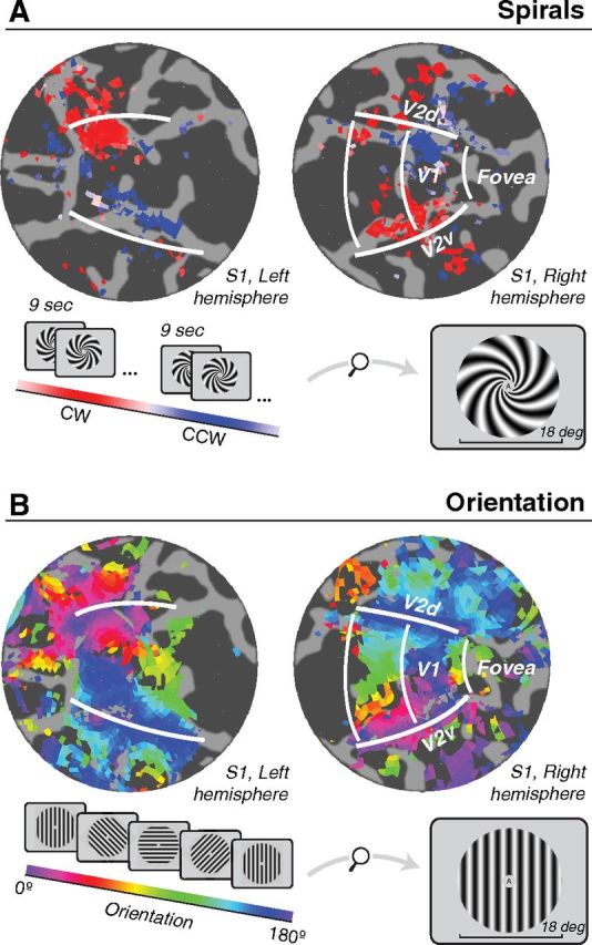
fMRI responses to spiral gratings and oriented gratings for an example subject (S1, same subject as shown in Fig. 3). A, Spirals alternated every 9 s between clockwise and counter-clockwise (inset). B, Oriented gratings cycled through 16 orientation steps ranging from 0° to 180° every 24 s. Responses from both experiments are shown on flattened representations (flat maps) of the occipital lobe. Dark gray, sulci. Light gray, gyri. Colors, Phase of best-fitting sinusoid (see color bars). For oriented gratings, the phase of the best-fitting sinusoid indicated the orientation preference of the voxel. For spiral gratings, the match of the phase to 0° or 180° reflected its spiral sense preference. White lines, V1/V2 boundaries as determined from an independent retinotopic mapping experiment.
Predicting spiral sense preference from orientation preference.
Spiral sense preference was predicted by combining responses to oriented gratings with retinotopic maps (Fig. 1B), individually for each subject. First, responses to oriented gratings were used to measure an orientation tuning function for each voxel. Specifically, we averaged the fMRI response time series from each voxel across runs and across cycles within each run. This yielded response amplitudes for each of the 16 orientations (i.e., a voxel-based orientation tuning function; Serences et al., 2009). The tuning functions captured both the degree to which the preferred orientation of each voxel deviated from radial in its orientation tuning function. Second, we used pRF mapping to measure the location in the visual field that evoked the largest response in each voxel (i.e., the center of the population receptive field of the voxel). We computed analytically the local orientation of both clockwise and counter-clockwise spirals at that location. For a given location, the local orientation of a spiral is given as follows:
where θ is the polar angle in the visual field, and the parameter b (defined above) controls how tightly the spiral is “wound.” The orientation does not depend on eccentricity, only polar angle. This analytic expression for local spiral orientation depends on the geometry of the spiral, and ignores interactions between the spiral image and neuronal preferences for spatial frequency and phase. Ignoring phase was justified because we randomized phase during stimulus presentation. Although we measured pRF sizes for each voxel, we did not assess spatial frequency preferences, so there was no way to incorporate spatial frequency in predicting spiral sense preference. We linearly interpolated the orientation tuning functions (with circular boundary handling), separately for each voxel, to predict responses to the local orientations of the clockwise and counter-clockwise spirals. Finally, we computed the difference between the predicted responses to counter-clockwise spirals minus the predicted responses to clockwise spirals.
To compare these predictions to measurements of spiral sense preference, we computed a signed measure of response amplitude from the spiral experiment. The fMRI time series from each voxel was projected onto a unit-norm sinusoid having period matched to the stimulus alternation and temporal phase of π/2 (4.5 s); this phase offset yielded a sinusoid approximately matched to the typical peak response to counter-clockwise spirals, accounting for hemodynamic delay. The amplitude of the projection provided a signed value isolating the component of the time series reflecting responses to counter-clockwise (positive) or clockwise spirals (negative). This analysis procedure took full advantage of a priori knowledge of the periodic experimental design (Heeger et al., 1999), and provided unbiased estimates of the amplitudes of response to the two kinds of spirals.
Accuracy of the spiral sense prediction was assessed as the correlation coefficient between the measured and predicted response amplitudes, separately for each voxel. Statistical significance of the predictions was assessed with a nonparametric randomization test. Specifically, we constructed a distribution of correlation coefficients expected under the null hypothesis that there was no relationship between the orientation preference of each voxel and the local spiral orientation. To generate this distribution, we randomly circularly shifted the orientation tuning function of each voxel before predicting its response to the spirals, and computed the correlation coefficient for this set of “randomly tuned” voxels. Repeating this procedure 1000 times yielded a distribution of correlations expected under the null hypothesis. The measured correlation coefficient (without randomization) was then compared with the null distribution; the proportion of the null distribution greater in magnitude than the measured value was designated as the (two-tailed) p value.
The correlation between measured and predicted spiral amplitude depends on (1) the reliability of the spiral responses, (2) the reliability of the prediction (which depends on the reliability of both pRF and orientation responses), (3) the accuracy of cross-registration across sessions, and (4) the accuracy of the model itself. Mathematically, the measured correlation is as follows:
 |
where rs is the reliability of the spiral measurements, rp is the reliability of the prediction, rsp is the estimated correlation, and rt is the true correlation, equal to 1 if cross-session registration and the model itself are perfect. By setting rt = 1, we can obtain an upper bound on rsp by estimating rs and rp. To estimate rs, we analyzed the spiral response amplitudes from the data collected in the first and second halves of each session. To estimate rp, we generated predictions of spiral response amplitude based on pRF and orientation data collected in the first and second halves of each session. Their geometric product provided an upper bound on rsp.
Decoding spiral sense.
Spiral sense was decoded from the responses to spiral gratings. Each run of the experiment consisted of 14 cycles of alternations between clockwise and counter-clockwise spirals. For each run, we averaged across cycles to yield a “cycle-averaged” response time series. We measured the response amplitudes for clockwise spirals as the average of frames 2–5 (3–7.5 s), and likewise frames 8–11 (12–16.5 s) for counter-clockwise spirals. This yielded two response amplitudes for each voxel in each run. Data from all runs were combined into an m × n matrix, with m being the number of voxels in V1, and n being the number of repeated measurements in the session (between 20 and 28: 2 response amplitudes for the 2 spiral senses × between 10 and 14 runs per session).
Decoding was performed with a maximum likelihood classifier, using the Matlab function “classify” with the option “diagLinear,” as described in detail previously (Brouwer and Heeger, 2009; Freeman et al., 2011). Accuracy was computed using split-halves cross-validation. The m × n data matrix was randomly partitioned along the n dimension (repeated measurements) into training and testing sets, with each containing an equal number of runs. Data in the training and testing sets were drawn from different runs in the same session and were thus statistically independent. The training set was used to estimate the parameters (multivariate means and variances) of the maximum-likelihood classifier. The testing set was then used for decoding. Decoding accuracy was determined as the proportion of the test examples that the classifier was able to assign to the correct spiral sense. We computed the median decoding accuracy across 1000 different partitions into training and testing.
A nonparametric randomization test was used to determine the statistical significance of decoding accuracy. Specifically, we constructed a distribution of accuracies expected under the null hypothesis that there was no relationship between the sense of the spiral stimulus and the corresponding responses. To generate this null distribution, we randomly permuted the spiral sense labels (i.e., clockwise and counter-clockwise) across runs in each scanning session, but using the same relabeling for all voxels in each run, and then recalculated the decoding accuracies. Repeating this randomization 10,000 times yielded a distribution of decoding accuracies expected under the null hypothesis. Statistical significance was assessed as the proportion of this distribution exceeding the accuracy computed with the correct labels (one tailed).
Spiral preference-based averaging.
This analysis determined whether the prediction of spiral sense preference was sufficient for spiral sense decoding. Statistically independent spiral sense predictions, generated from independent orientation and pRF estimates, were used to assign each voxel to one of two groups, corresponding to voxels predicted to prefer CW or CCW spirals. These two groups were further subdivided based on the amplitude of the predicted spiral preference, with 10 evenly spaced bins on a log scale ranging from 0.1 to 2.0% change in image intensity. We averaged the time series from the spiral experiment of all voxels within each bin, yielding “supervoxels,” which were then used for spiral decoding. The decoding achieved by each pair of supervoxels was compared against decoding using a “random” pair of supervoxels containing the same number of individual voxels, but chosen at random (with multiple draws of random voxels).
Z-offset experiment.
An additional experiment measured the impact of directly manipulating the spatial relationship between the fMRI voxel grid and the underlying columnar organization for orientation. In this experiment, we shifted the fMRI slices by half a voxel (1 mm), orthogonal to the x–y plane of the image acquisition, for the even-numbered runs in each scanning session (i.e., so that each slice from the even-numbered runs was centered between slices from the odd-numbered runs). We trained a classifier (as above) with data from either the odd- or even-numbered runs, and tested the classifier with data from either the odd- or even-numbered runs (i.e., corresponding to the same or different slice positions). Specifically, we trained the classifier on data from run 1 (unshifted slices) and separately tested the classifier on run 2 (shifted slices) and run 3 (unshifted slices). We repeated this for each set of three consecutive runs (e.g., training on run 2, testing on runs 3 and 4, and so on). This procedure yielded a set of decoding accuracies for training/testing with the same slice position versus training/testing with different slice positions. We ran this experiment with the same stimuli (spiral gratings and oriented gratings) and task as in the main experiment.
Eyetracking.
Eye position was monitored at 1000 Hz during fMRI scanning with a high-resolution eyetracker (MR-compatible EyeLink 1000). Eye position traces were analyzed off-line to ensure that subjects were fixating the intended location. Large saccades away from the fixation cross were rare, typically occurring not more than once per run, if at all. Subjects made microsaccades (i.e., involuntary saccades <1°), but neither microsaccade rate nor microsaccade direction varied systemically with spiral sense (data not shown).
Results
Coarse-scale responses to spirals in human visual cortex
A coarse-scale pattern of differential responses to spirals was observed in V1 (and to some extent V2) in multiple subjects (example shown in Fig. 2A, subject S1). These spiral sense preferences exhibited a quadrant-like organization. In the ventral portion of the right hemisphere (corresponding retinotopically to the top left visual field quadrant), there was a preference for clockwise spirals. In the dorsal portion of the right hemisphere, there was a preference for counter-clockwise spirals. The pattern was reversed in the left hemisphere: clockwise spirals were preferred in dorsal V1 (bottom right visual field) and counter-clockwise in ventral V1 (top right visual field). Not all subjects showed this exact pattern, but each showed reliable coarse-scale spiral preferences that depended on left versus right and/or upper versus lower visual field.
Given these coarse-scale spiral sense preferences, we were able to decode spiral sense using the multivariate pattern of voxel responses in V1, replicating previous findings for glass-pattern spirals (Mannion et al., 2009). Decoding accuracy was high in each of six hemispheres from three subjects (mean ± SE across hemispheres, 96 ± 0.26%; p < 0.05, randomization test computed separately for each hemisphere). We averaged the responses across voxels within each retinotopically defined visual quadrant and repeated the classification analysis; accuracy was still well above chance in five of six hemispheres (81 ± 5.6%; p < 0.05, randomization test). However, when we averaged responses randomly, without regard to the retinotopic selectivity of each voxel, decoding accuracy was not significantly above chance in five of six hemispheres (61 ± 4.7%, randomization test). This implies that the coarse-scale spiral sense preferences (at the scale of entire visual quadrants) were sufficient for accurate decoding.
Relating orientation and spiral preferences
If orientation biases in V1 are primarily radial, why are there robust differential responses to clockwise and counter-clockwise spirals? Coarse-scale biases for radial orientations have been well documented in human V1 (Sasaki et al., 2006; Freeman et al., 2011), but radial biases have been most robustly documented in the periphery. Orientation preferences near the fovea may be closer to vertical or near-vertical (Freeman et al., 2011). If, at any location within V1, a voxel has an orientation bias that is not precisely radial, it will prefer one spiral more than the other, and the spiral sense preference will depend on the orientation bias (Fig. 1A). Furthermore, if the nonradial bias has a coarse spatial scale (e.g., a consistent preference for near-vertical orientations near the fovea, as previously documented), it could yield coarse-scale preferences for spiral sense.
To investigate whether a nonradial orientation bias might predict responses to spirals, we compared responses to orientated gratings and spirals in the same subjects (Figs. 3, 4; see Materials and Methods). As described previously (Freeman et al., 2011), orientation preferences exhibited coarse-scale organization (Fig. 2B). Orientation preferences and population receptive fields together were used to predict spiral sense preferences for each voxel (see Materials and Methods; Fig. 1B). Measured spiral sense preferences were qualitatively similar to the predicted spiral sense preferences (Fig. 3). Correlations between predicted and measured spiral sense preferences were statistically significant in all three individual subjects (Fig. 4; S1, r = 0.38; S2, r = 0.46; S3, r = 0.39; all p < 0.0001, randomization test). These correlations were lower than a theoretical upper bound (r = 0.65 ± 0.15, mean ± SD; n = 3 subjects), derived from the reliability of the measured fMRI responses (see Materials and Methods). However, the upper bound assumed that cross-session registration was perfect, and that the predictions were limited only by within-session measurement noise.
Figure 3.

Measured and predicted spiral sense preferences for an example subject (S1, same subject shown in Fig. 2). A, Measured spiral sense preference. B, Predicted spiral sense preference, computed from measurements of orientation preference and population receptive field location (see also Fig. 1B). Each point corresponds to a single voxel, plotted in the visual field based on its estimated population receptive field location. Color (red or blue) indicates the preferred spiral sense (clockwise or counter-clockwise). Symbol size and saturation indicates the difference in response amplitudes (either measured or predicted) to the two spirals. Although the experimental stimulus subtended 18° (9° radius), the plot has been cropped slightly to emphasize the region of the visual field where spiral responses were strongest.
Figure 4.

Measured and predicted responses to spirals, for all three subjects (including subject S1, also shown in Figs. 1, 2). Ordinate, fMRI response amplitudes measured in the spiral experiment, during which stimuli alternated between clockwise and counter-clockwise; abscissa, predicted response amplitudes derived jointly from orientation preferences and population receptive fields. Each point corresponds to a voxel. Symbol size indicates the measured spiral sense preference (difference in response amplitudes to the two spirals).
The spiral sense preferences were driven primarily by nonradial orientation preferences near the fovea (Fig. 5). We compared the polar angle of the population receptive field of each voxel to its orientation preference and its spiral sense preference. At larger eccentricities (>5°), most voxels exhibited a radial bias (Fig. 5B, data points near diagonal), and most did not exhibit strong spiral sense preferences (Fig. 5B, light red and light blue). At smaller eccentricities (<5°), most voxels exhibited near-vertical (i.e., nonradial) orientation preferences (Fig. 5A, data points near 0° and 180° on the y-axis), and most had strong spiral sense preferences (Fig. 5A, dark red and dark blue). A small subset of voxels near the vertical meridian preferred vertical (i.e., radial) orientation, but still showed strong spiral sense preferences (Fig. 5A, dark red and dark blue data points near the diagonal). We speculate that this might be an artifact due to the difficulty of measuring population receptive fields at the vertical meridian (Binda et al., 2013).
Figure 5.

Spiral sense preferences arise from nonradial orientation preferences near the fovea. Both panels plot the orientation preference versus the polar angle component of the population receptive field. Each data point corresponds to a single voxel. Color (red or blue) indicates spiral sense preference (clockwise or counter-clockwise, respectively). Symbol size and saturation indicates the difference in response amplitudes to the two spirals. A, Voxels for which the radial component of the population receptive field is <5°. B, Voxels for which the radial component of the population receptive field is >5°.
Coarse-scale bias is sufficient for decoding both orientation and spiral sense
The relationship between orientation preferences and spiral sense preferences was further quantified, following our previous work (Freeman et al., 2011), by determining whether orientation and retinotopic preferences were sufficient for spiral decoding (Fig. 6). We measured the decoding accuracy for pairs of supervoxels, created by averaging the time series from voxels that were selected based on the spiral sense prediction. Voxels were sorted into two groups based on their predicted spiral sense preference for CCW or CW. Each of the two groups was subdivided into 10 bins based on the degree of predicted selectivity for CCW and CW spirals, and then averaged. For pairs of supervoxels (one for each spiral sense) in which the predicted selectivity was low, spiral sense decoding was at chance (relative to a null distribution computed by randomly sorting voxels into two groups). For supervoxels in which the predicted spiral sense selectivity was high, decoding was near perfect, well above the accuracy obtained by creating supervoxels from randomly selected voxels.
Figure 6.

Orientation and retinotopic preferences were sufficient for spiral decoding. Black symbols, Decoding accuracy for pairs of supervoxels, created by averaging the time series from voxels that were selected based on the spiral sense prediction. Voxels sorted into two groups based on their predicted spiral sense preference for CCW or CW. Each of the two groups was subdivided into 10 bins based on the degree of predicted selectivity for CCW and CW spirals, and then averaged. Gray symbols, Voxels were assigned to bins randomly, not based on the spiral sense prediction. Error bars indicate SEM across three subjects (n = 3).
An independent experiment confirmed that coarse-scale bias was sufficient for both orientation and spiral sense decoding (Fig. 7). We repeated the experiments with spiral gratings and oriented gratings, but shifted the slices by half a voxel (1 mm) on alternate runs (Fig. 6). Subjects were scanned in 12–14 runs per session. We trained and tested a classifier on runs in which the slices were either in the same spatial position (Fig. 7A, green) or in different positions (Fig. 7A, blue). Shifting the slices changed the relationship between the underlying columnar architecture and the region of cortex sampled by each fMRI voxel. Hypercolumns in human visual cortex are ∼2 mm (Adams et al., 2007), and the slices were oriented approximately perpendicular to the calcarine sulcus, so the 1 mm offset shifted gray matter voxels by about half a hypercolumn. Decoding accuracy would have been reduced if fine-scale cortical information had a considerable impact on the fMRI responses. But, we found no difference in decoding accuracy between shifted slices and unshifted slices (Fig. 7B). Decoding accuracy was nearly perfect for spiral sense decoding, raising concern that we might not be sensitive to any possible decrements in decoding accuracy with shifted slices. This concern was ruled out by the orientation-decoding results, for which decoding accuracy was well below ceiling.
Figure 7.

Coarse-scale bias is sufficient for decoding both orientation and spiral sense. Slices were shifted by half a voxel (1 mm) on even-numbered runs. A, Measured slice position for each temporal frame of each scan, from one example scanning session. Slice position was measured using a robust image registration algorithm (Nestares and Heeger, 2000). B, Decoding accuracies when the classifier was trained and tested with data from either the same (green) or different (blue) slice positions (mean of two subjects).
Discussion
We used fMRI to show that both oriented gratings and logarithmic spirals evoked coarse-scale patterns of activity in human V1. Orientation preferences were radial in the V1 representation of the periphery and near-vertical closer to the fovea. Spiral sense preferences varied systematically across V1 representations of the visual field quadrants. Orientation preferences predicted responses to spiral stimuli across independent experiments, suggesting that a robust orientation bias underlies responses to both oriented gratings and spirals. The coarse-scale bias for orientation was sufficient for decoding both orientation and spiral sense.
We have used the terms “coarse-scale” to indicate a topography in stimulus preference that bears a systematic relationship to the retinotopic organization (∼1 cm), and “fine-scale” to indicate a variation in stimulus preference that bears a systematic relationship to the columnar architecture (∼1 mm). These operational definitions are suitable in visual cortex, where retinotopic-scale and columnar-scale organizations are well established. But a more fundamental notion of the scale of cortical topography would be useful in other domains.
The fine-scale representation of orientation in V1 has been studied extensively (Hubel and Wiesel, 1959), but the neurophysiological basis of coarse-scale biases for orientations and spirals remain unknown. Both radial and nonradial biases in V1 could be entirely inherited from earlier stages of visual processing. The retina and LGN both exhibit radial biases in receptive field shape (Levick and Thibos, 1980, 1982; Rodieck et al., 1985; Schall et al., 1986; Shou et al., 1986; Smith et al., 1990). The biases in the retina might be related to axon trajectories (Airaksinen et al., 2008) instead of, or in addition to, retinotopic location per se, and thus only radial in some regions of the visual field (E. J. Chichilnisky, personal communication). Models of orientation selectivity based on retinal anatomy and feedforward connectivity (Ringach, 2007) predict a correspondence between biases in receptive field shape in the retina and LGN, and biases for orientation preference in V1. But orientation biases in V1 might also reflect processing within V1. Multielectrode recordings in V1 have revealed a signal in the gamma band of the local field potential (LFP) that is orientation tuned, consistent across millimeters of cortex, and dissociated from local spiking activity (Jia et al., 2011). But it is not yet known whether this LFP signal exhibits the same coarse-scale topography that we have measured with fMRI.
Some theories of visual processing posit that orientation preferences in V1 might depend on, or vary with, the global properties of the stimulus (e.g., whether it is a grating or a spiral). Such variation in sensory encoding could arise, for example, due to feedback from downstream areas selective for global shape (Pasupathy and Connor, 2002; Ostwald et al., 2008; Williams et al., 2008; Mannion et al., 2010b; Mannion and Clifford, 2011) or from differences in attention to the different kinds of stimuli (Wannig et al., 2011). However, we were able to predict responses to one type of large pattern (spirals) by measuring responses to another type of large pattern (grating), implying that the orientation preference of a voxel generalizes between stimuli and is robust to differences in global context.
The ability to decode spiral sense replicates and extends previous studies (Mannion et al., 2009), but we reached a different conclusion. Previous studies assumed only a coarse-scale radial bias, so the ability to decode radially matched spirals was interpreted as implying a fine-scale, columnar contribution to selectivity for orientation. However, this logic only applies if the coarse-scale orientation bias is precisely radial across the entire visual field. Our results demonstrate a bias for local stimulus orientation, which has a coarse spatial scale; is robust across stimulus classes (spirals and gratings); and suffices to explain decoding from fMRI responses in V1.
Still open is the question of whether fMRI can reflect signals originating from sampling random irregularities in the fine-scale columnar architecture. There is a columnar architecture in human visual cortex (Adams et al., 2007), so BOLD fMRI measurements at conventional resolution (≥2 × 2 × 2 mm) might reflect a combination of fine-scale and coarse-scale contributions. Our finding that the decoding of both orientation and spiral sense were unaffected by shifting slices between collecting data for training and testing the classifier, together with our demonstrations of coarse-scale biases for orientation and spiral sense, provide evidence that the overwhelming majority of the signal is coarse scale. Many other efforts have taken as a starting point that fine-scale signals underlie the ability to decode orientation. This conjecture would be more forceful if there was more positive evidence in its favor. For example, it is possible to measure orientation columns with high-resolution, high-field strength BOLD fMRI (Zhao et al., 2005; Uğurbil, 2012). Particularly convincing would be a comparison between decoding accuracies after downsampling these high-resolution measurements to conventional scanning resolutions, with and without first removing the columnar-scale signals completely via regression (Freeman et al., 2011).
Topographic organization is evident throughout the sensory nervous system at multiple spatial scales, including maps of visual location (Wandell et al., 2007), orientation (Ohki et al., 2006; Sasaki et al., 2006; Freeman et al., 2011), speed (Nishimoto et al., 2011), motion direction (Beckett et al., 2012), object preference (Huth et al., 2012; Konkle and Oliva, 2012; Issa et al., 2013), and place (Moser et al., 2008). However, the behavioral importance of topographic organization is not well understood. The coarse-scale biases we observed for both orientation and spirals might reflect the morphology or development of the visual system. They might instead, or in addition, arise from the statistics of orientation in natural images (Girshick et al., 2011), which are known to vary across the visual field (Rothkopf and Ballard, 2009).
Footnotes
This research was supported by National Institutes of Health Grants R01-EY019693 (D.J.H.), RO1-EY022398 (D.J.H.), and R01-NS047493 (E.P.M. and D.J.H.); and by a National Science Foundation Graduate Student Fellowship (J.F.). We thank Corey M. Ziemba for helpful suggestions.
References
- Adams DL, Sincich LC, Horton JC. Complete pattern of ocular dominance columns in human primary visual cortex. J Neurosci. 2007;27:10391–10403. doi: 10.1523/JNEUROSCI.2923-07.2007. [DOI] [PMC free article] [PubMed] [Google Scholar]
- Airaksinen PJ, Doro S, Veijola J. Conformal geometry of the retinal nerve fiber layer. Proc Natl Acad Sci U S A. 2008;105:19690–19695. doi: 10.1073/pnas.0801621105. [DOI] [PMC free article] [PubMed] [Google Scholar]
- Alink A, Krugliak A, Walther A, Kriegeskorte N. fMRI orientation decoding in V1 does not require global maps or globally coherent orientation stimuli. Front Psychol. 2013;4:493. doi: 10.3389/fpsyg.2013.00493. [DOI] [PMC free article] [PubMed] [Google Scholar]
- Beckett A, Peirce JW, Sanchez-Panchuelo RM, Francis S, Schluppeck D. Contribution of large scale biases in decoding of direction-of-motion from high-resolution fMRI data in human early visual cortex. Neuroimage. 2012;63:1623–1632. doi: 10.1016/j.neuroimage.2012.07.066. [DOI] [PubMed] [Google Scholar]
- Binda P, Thomas JM, Boynton GM, Fine I. Minimizing biases in estimating the reorganization of human visual areas with BOLD retinotopic mapping. J Vis. 2013;13(7):13, 1–16. doi: 10.1167/13.7.13. [DOI] [PMC free article] [PubMed] [Google Scholar]
- Boynton GM. Imaging orientation selectivity: decoding conscious perception in V1. Nat Neurosci. 2005;8:541–542. doi: 10.1038/nn0505-541. [DOI] [PubMed] [Google Scholar]
- Brouwer GJ, Heeger DJ. Decoding and reconstructing color from responses in human visual cortex. J Neurosci. 2009;29:13992–14003. doi: 10.1523/JNEUROSCI.3577-09.2009. [DOI] [PMC free article] [PubMed] [Google Scholar]
- Clifford CWG, Mannion DJ, Seymour KJ, McDonald JS, Bartels A. Are coarse-scale orientation maps really necessary for orientation decoding? J Neurosci. 2011. Available at http://www.jneurosci.org/content/31/13/4792/reply.
- Dumoulin SO, Wandell BA. Population receptive field estimates in human visual cortex. Neuroimage. 2008;39:647–660. doi: 10.1016/j.neuroimage.2007.09.034. [DOI] [PMC free article] [PubMed] [Google Scholar]
- Engel SA, Glover GH, Wandell BA. Retinotopic organization in human visual cortex and the spatial precision of functional MRI. Cereb Cortex. 1997;7:181–192. doi: 10.1093/cercor/7.2.181. [DOI] [PubMed] [Google Scholar]
- Freeman J, Brouwer GJ, Heeger DJ, Merriam EP. Orientation decoding depends on maps, not columns. J Neurosci. 2011;31:4792–4804. doi: 10.1523/JNEUROSCI.5160-10.2011. [DOI] [PMC free article] [PubMed] [Google Scholar]
- Furmanski CS, Engel SA. An oblique effect in human primary visual cortex. Nat Neurosci. 2000;3:535–536. doi: 10.1038/75702. [DOI] [PubMed] [Google Scholar]
- Gardner JL. Is cortical vasculature functionally organized? Neuroimage. 2010;49:1953–1956. doi: 10.1016/j.neuroimage.2009.07.004. [DOI] [PubMed] [Google Scholar]
- Gardner JL, Merriam EP, Movshon JA, Heeger DJ. Maps of visual space in human occipital cortex are retinotopic, not spatiotopic. J Neurosci. 2008;28:3988–3999. doi: 10.1523/JNEUROSCI.5476-07.2008. [DOI] [PMC free article] [PubMed] [Google Scholar]
- Girshick AR, Landy MS, Simoncelli EP. Cardinal rules: visual orientation perception reflects knowledge of environmental statistics. Nat Neurosci. 2011;14:926–932. doi: 10.1038/nn.2831. [DOI] [PMC free article] [PubMed] [Google Scholar]
- Haynes JD, Rees G. Predicting the orientation of invisible stimuli from activity in human primary visual cortex. Nat Neurosci. 2005;8:686–691. doi: 10.1038/nn1445. [DOI] [PubMed] [Google Scholar]
- Heeger DJ, Boynton GM, Demb JB, Seidemann E, Newsome WT. Motion opponency in visual cortex. J Neurosci. 1999;19:7162–7174. doi: 10.1523/JNEUROSCI.19-16-07162.1999. [DOI] [PMC free article] [PubMed] [Google Scholar]
- Hubel D, Wiesel T. Receptive fields of single neurones in the cat's striate cortex. J Physiol. 1959;148:574–591. doi: 10.1113/jphysiol.1959.sp006308. [DOI] [PMC free article] [PubMed] [Google Scholar]
- Huth AG, Nishimoto S, Vu AT, Gallant JL. A continuous semantic space describes the representation of thousands of object and action categories across the human brain. Neuron. 2012;76:1210–1224. doi: 10.1016/j.neuron.2012.10.014. [DOI] [PMC free article] [PubMed] [Google Scholar]
- Issa EB, Papanastassiou AM, DiCarlo JJ. Large-scale, high-resolution neurophysiological maps underlying fMRI of macaque temporal lobe. J Neurosci. 2013;33:15207–15219. doi: 10.1523/JNEUROSCI.1248-13.2013. [DOI] [PMC free article] [PubMed] [Google Scholar]
- Jia X, Smith MA, Kohn A. Stimulus selectivity and spatial coherence of gamma components of the local field potential. J Neurosci. 2011;31:9390–9403. doi: 10.1523/JNEUROSCI.0645-11.2011. [DOI] [PMC free article] [PubMed] [Google Scholar]
- Kamitani Y, Sawahata Y. Spatial smoothing hurts localization but not information: pitfalls for brain mappers. Neuroimage. 2010;49:1949–1952. doi: 10.1016/j.neuroimage.2009.06.040. [DOI] [PubMed] [Google Scholar]
- Kamitani Y, Tong F. Decoding the visual and subjective contents of the human brain. Nat Neurosci. 2005;8:679–685. doi: 10.1038/nn1444. [DOI] [PMC free article] [PubMed] [Google Scholar]
- Konkle T, Oliva A. A real-world size organization of object responses in occipitotemporal cortex. Neuron. 2012;74:1114–1124. doi: 10.1016/j.neuron.2012.04.036. [DOI] [PMC free article] [PubMed] [Google Scholar]
- Kriegeskorte N, Cusack R, Bandettini P. How does an fMRI voxel sample the neuronal activity pattern: compact-kernel or complex spatiotemporal filter? Neuroimage. 2010;49:1965–1976. doi: 10.1016/j.neuroimage.2009.09.059. [DOI] [PMC free article] [PubMed] [Google Scholar]
- Larsson J, Heeger DJ. Two retinotopic visual areas in human lateral occipital cortex. J Neurosci. 2006;26:13128–13142. doi: 10.1523/JNEUROSCI.1657-06.2006. [DOI] [PMC free article] [PubMed] [Google Scholar]
- Levick WR, Thibos LN. Orientation bias of cat retinal ganglion cells. Nature. 1980;286:389–390. doi: 10.1038/286389a0. [DOI] [PubMed] [Google Scholar]
- Levick WR, Thibos LN. Analysis of orientation bias in cat retina. J Physiol. 1982;329:243–261. doi: 10.1113/jphysiol.1982.sp014301. [DOI] [PMC free article] [PubMed] [Google Scholar]
- Mannion DJ, McDonald JS, Clifford CW. Discrimination of the local orientation structure of spiral Glass patterns early in human visual cortex. Neuroimage. 2009;46:511–515. doi: 10.1016/j.neuroimage.2009.01.052. [DOI] [PubMed] [Google Scholar]
- Mannion DJ, McDonald JS, Clifford CW. Orientation anisotropies in human visual cortex. J Neurophysiol. 2010a;103:3465–3471. doi: 10.1152/jn.00190.2010. [DOI] [PubMed] [Google Scholar]
- Mannion DJ, McDonald JS, Clifford CW. The influence of global form on local orientation anisotropies in human visual cortex. Neuroimage. 2010b;52:600–605. doi: 10.1016/j.neuroimage.2010.04.248. [DOI] [PubMed] [Google Scholar]
- Mannion DJ, Clifford CWG. Cortical and behavioral sensitivity to eccentric polar form. J Vis. 2011;11(6):17, 1–9. doi: 10.1167/11.6.17. [DOI] [PubMed] [Google Scholar]
- Moser EI, Kropff E, Moser MB. Place cells, grid cells, and the brain's spatial representation system. Annu Rev Neurosci. 2008;31:69–89. doi: 10.1146/annurev.neuro.31.061307.090723. [DOI] [PubMed] [Google Scholar]
- Nestares O, Heeger DJ. Robust multiresolution alignment of MRI brain volumes. Magn Reson Med. 2000;43:705–715. doi: 10.1002/(SICI)1522-2594(200005)43:5<705::AID-MRM13>3.0.CO%3B2-R. [DOI] [PubMed] [Google Scholar]
- Nishimoto S, Vu AT, Naselaris T, Benjamini Y, Yu B, Gallant JL. Reconstructing visual experiences from brain activity evoked by natural movies. Curr Biol. 2011;21:1641–1646. doi: 10.1016/j.cub.2011.08.031. [DOI] [PMC free article] [PubMed] [Google Scholar]
- Ogawa S, Lee TM, Kay AR, Tank DW. Brain magnetic resonance imaging with contrast dependent on blood oxygenation. Proc Natl Acad Sci U S A. 1990;87:9868–9872. doi: 10.1073/pnas.87.24.9868. [DOI] [PMC free article] [PubMed] [Google Scholar]
- Ohki K, Chung S, Kara P, Hübener M, Bonhoeffer T, Reid RC. Highly ordered arrangement of single neurons in orientation pinwheels. Nature. 2006;442:925–928. doi: 10.1038/nature05019. [DOI] [PubMed] [Google Scholar]
- Op de Beeck HP. Probing the mysterious underpinnings of multi-voxel fMRI analyses. Neuroimage. 2010a;50:567–571. doi: 10.1016/j.neuroimage.2009.12.072. [DOI] [PubMed] [Google Scholar]
- Op de Beeck HP. Against hyperacuity in brain reading: spatial smoothing does not hurt multivariate fMRI analyses? Neuroimage. 2010b;49:1943–1948. doi: 10.1016/j.neuroimage.2009.02.047. [DOI] [PubMed] [Google Scholar]
- Ostwald D, Lam JM, Li S, Kourtzi Z. Neural coding of global form in the human visual cortex. J Neurophysiol. 2008;99:2456–2469. doi: 10.1152/jn.01307.2007. [DOI] [PubMed] [Google Scholar]
- Pasupathy A, Connor CE. Population coding of shape in area V4. Nat Neurosci. 2002;5:1332–1338. doi: 10.1038/nn972. [DOI] [PubMed] [Google Scholar]
- Ress D, Backus BT, Heeger DJ. Activity in primary visual cortex predicts performance in a visual detection task. Nat Neurosci. 2000;3:940–945. doi: 10.1038/78856. [DOI] [PubMed] [Google Scholar]
- Ringach DL. On the origin of the functional architecture of the cortex. PLoS One. 2007;2:e251. doi: 10.1371/journal.pone.0000251. [DOI] [PMC free article] [PubMed] [Google Scholar]
- Rodieck RW, Binmoeller KF, Dineen J. Parasol and midget ganglion cells of the human retina. J Comp Neurol. 1985;233:115–132. doi: 10.1002/cne.902330107. [DOI] [PubMed] [Google Scholar]
- Rothkopf CA, Ballard DH. Image statistics at the point of gaze during human navigation. Vis Neurosci. 2009;26:81–92. doi: 10.1017/S0952523808080978. [DOI] [PMC free article] [PubMed] [Google Scholar]
- Sasaki Y, Rajimehr R, Kim BW, Ekstrom LB, Vanduffel W, Tootell RB. The radial bias: a different slant on visual orientation sensitivity in human and nonhuman primates. Neuron. 2006;51:661–670. doi: 10.1016/j.neuron.2006.07.021. [DOI] [PubMed] [Google Scholar]
- Schall JD, Vitek DJ, Leventhal AG. Retinal constraints on orientation specificity in cat visual cortex. J Neurosci. 1986;6:823–836. doi: 10.1523/JNEUROSCI.06-03-00823.1986. [DOI] [PMC free article] [PubMed] [Google Scholar]
- Serences JT, Saproo S, Scolari M, Ho T, Muftuler LT. Estimating the influence of attention on population codes in human visual cortex using voxel-based tuning functions. Neuroimage. 2009;44:223–231. doi: 10.1016/j.neuroimage.2008.07.043. [DOI] [PubMed] [Google Scholar]
- Shmuel A, Chaimow D, Raddatz G, Ugurbil K, Yacoub E. Mechanisms underlying decoding at 7 T: ocular dominance columns, broad structures, and macroscopic blood vessels in V1 convey information on the stimulated eye. Neuroimage. 2010;49:1957–1964. doi: 10.1016/j.neuroimage.2009.08.040. [DOI] [PMC free article] [PubMed] [Google Scholar]
- Shou T, Ruan D, Zhou Y. The orientation bias of LGN neurons shows topographic relation to area centralis in the cat retina. Exp Brain Res. 1986;64:233–236. doi: 10.1007/BF00238218. [DOI] [PubMed] [Google Scholar]
- Smith EL, 3rd, Chino YM, Ridder WH, 3rd, Kitagawa K, Langston A. Orientation bias of neurons in the lateral geniculate nucleus of macaque monkeys. Vis Neurosci. 1990;5:525–545. doi: 10.1017/S0952523800000699. [DOI] [PubMed] [Google Scholar]
- Smith AM, Lewis BK, Ruttimann UE, Ye FQ, Sinnwell TM, Yang Y, Duyn JH, Frank JA. Investigation of low frequency drift in fMRI signal. Neuroimage. 1999;9:526–533. doi: 10.1006/nimg.1999.0435. [DOI] [PubMed] [Google Scholar]
- Swisher JD, Gatenby JC, Gore JC, Wolfe BA, Moon CH, Kim SG, Tong F. Multiscale pattern analysis of orientation-selective activity in the primary visual cortex. J Neurosci. 2010;30:325–330. doi: 10.1523/JNEUROSCI.4811-09.2010. [DOI] [PMC free article] [PubMed] [Google Scholar]
- Tong F, Pratte MS. Decoding patterns of human brain activity. Annu Rev Psychol. 2012;63:483–509. doi: 10.1146/annurev-psych-120710-100412. [DOI] [PMC free article] [PubMed] [Google Scholar]
- Uğurbil K. The road to functional imaging and ultrahigh fields. Neuroimage. 2012;62:726–735. doi: 10.1016/j.neuroimage.2012.01.134. [DOI] [PMC free article] [PubMed] [Google Scholar]
- Wandell BA, Dumoulin SO, Brewer AA. Visual field maps in human cortex. Neuron. 2007;56:366–383. doi: 10.1016/j.neuron.2007.10.012. [DOI] [PubMed] [Google Scholar]
- Wannig A, Stanisor L, Roelfsema PR. Automatic spread of attentional response modulation along Gestalt criteria in primary visual cortex. Nat Neurosci. 2011;14:1243–1244. doi: 10.1038/nn.2910. [DOI] [PubMed] [Google Scholar]
- Williams MA, Baker CI, Op de Beeck HP, Shim WM, Dang S, Triantafyllou C, Kanwisher N. Feedback of visual object information to foveal retinotopic cortex. Nat Neurosci. 2008;11:1439–1445. doi: 10.1038/nn.2218. [DOI] [PMC free article] [PubMed] [Google Scholar]
- Zhao F, Wang P, Hendrich K, Kim SG. Spatial specificity of cerebral blood volume-weighted fMRI responses at columnar resolution. Neuroimage. 2005;27:416–424. doi: 10.1016/j.neuroimage.2005.04.011. [DOI] [PubMed] [Google Scholar]