Is DNA a Good Model Polymer?

Abstract

The details surrounding the cross-over from wormlike-specific to universal polymeric behavior has been the subject of debate and confusion even for the simple case of a dilute, unconfined wormlike chain. We have directly computed the polymer size, form factor, free energy and Kirkwood diffusivity for unconfined wormlike chains as a function of molecular weight, focusing on persistence lengths and effective widths that represent single-stranded and double-stranded DNA in a high ionic strength buffer. To do so, we use a chain-growth Monte Carlo algorithm, the Pruned-Enriched Rosenbluth Method (PERM), which allows us to estimate equilibrium and near-equilibrium dynamic properties of wormlike chains over an extremely large range of contour lengths. From our calculations, we find that very large DNA chains (≈ 1,000,000 base pairs depending on the choice of size metric) are required to reach flexible, swollen non-draining coils. Furthermore, our results indicate that the commonly used model polymer λ-DNA (48,500 base pairs) does not exhibit “ideal” scaling, but exists in the middle of the transition to long-chain behavior. We subsequently conclude that typical DNA used in experiments are too short to serve as an accurate model of long-chain, universal polymer behavior.

1 Introduction

Double-stranded DNA (dsDNA) has long stood as a unique polymer due to its role in biology and biochemistry. In addition, thanks to modern techniques in molecular biology and soft-matter physics, monodisperse samples of dsDNA can be prepared with an extraordinarily large range of molecular weights, which can in turn be visualized and controlled at the single-molecule level. Accordingly, dsDNA has assumed the role of a “model polymer” and has been extensively studied. Despite its widespread use, accumulating evidence suggests that dsDNA is not a good model polymer for investigating universal polymer properties, and a version of the more flexible single-stranded DNA (ssDNA) with limited base pair interactions has been proposed as an alternative.^1,2 In this paper, we examine the length-dependent properties of both single-stranded and double-stranded DNA in order to further evaluate their fitness as model polymers.

In order to do so, we first ask why any specific polymer would be an appropriate general model in the first place? The answer is given by the aptly named concept of universality, which was well explained by de Gennes.³ Universality implies that at sufficiently large length (and time) scales, all dilute solutions of self-avoiding polymers in a good solvent exhibit equivalent behavior, regardless of disparate underlying chemical structures.^3–5 Therefore at large enough contour lengths all polymers are “model” polymers, because all polymers behave similarly (e.g. entropic elasticity and self-avoidance). This is certainly the sense in which dsDNA, ssDNA or any other polymer is meant as a model polymer.

Due to the specific chemical structure of dsDNA, its behavior is well described by the worm-like chain model,⁶ and at short enough length scales (near the persistence length) dsDNA is often described as semiflexible. Accordingly, it is sometimes repeated that “dsDNA is not a good model of flexible molecules, because it is semiflexible”. However, this statement can lead to confusion due to an unfortunate ambiguity surrounding the word “semiflexible” that often arises in the literature. Per our definition of universality, this statement is correct if the term semiflexible is meant to denote a polymer with a contour length near its persistence length. Indeed, universality provides no basis for comparing any short-chain polymer to either another short-chain polymer of different chemistry or the general behavior of all polymers. Using this terminology, a flexible chain is thus any chain that shows universal behavior. However, if the term semiflexible is used as a synonym for the class of polymers that are well described by the Kratky-Porod model (i.e. wormlike chains), then this statement is incorrect since very long wormlike polymers indeed show universal behavior. The statement is all the more misleading because it implies that dsDNA is always semiflexible, which is true if semiflexible is synonymous with wormlike, but false if semiflexible means short. In this paper, we shall use the term “semiflexible chain” to denote a member of the class of wormlike chains.

Regardless of notational convention, the principle of universality immediately suggests a way to assess the theoretical appropriateness of a proposed model polymer. Namely, is the polymer long enough such that chemically specific behavior disappears? This of course completely neglects the bedrock question that made DNA the model polymer of choice: Is the model polymer experimentally convenient to use? For a polymer to serve as both a correct and practically useful model polymer, these two questions must be answered affirmatively. In this work, we purposefully omit any normative statements about experimental convenience, and instead compute the contour length where the chemically specific behavior of dsDNA disappears. In this way, we seek to quantify how both static (e.g. radius of gyration) and dynamic (e.g. diffusion coefficient) properties of dsDNA approach universal behavior. Along the way, we find it instructive to compare to the properties of a model of ssDNA as well.

There is a lack of consensus in the literature regarding the appropriate length at which one can consider dsDNA to be a flexible chain. For instance, some authors have claimed that even a very long molecule like λ-DNA is “ideal”, being too short and stiff to experience excluded volume interactions.^2,7 However other studies suggest that excluded volume interactions indeed have an impact at similar contour lengths.^8–10 Further confounding the issue, the oft-cited measurements of the diffusion coefficient of concatamers of λ-DNA by Smith et al.¹¹ suggested that dsDNA had already reached a universal limit. However, the work by Smith et al. is at odds with recent theoretical work on the draining behavior of wormlike polymer coils¹² and work on DNA in confinement¹³ which suggests that the molecular weight required to reach the universal limit for dynamic properties is even larger than the weight required for static properties.

Adding to the confusion, intercalating dyes, which make dsDNA so convenient to use in fluorescence microscopy experiments, have an undeniable impact on the chain chemistry of dsDNA — extending the molecular contour length by 20–30%.¹⁴ Even so, the most basic molecular properties of dyed dsDNA (i.e. the persistence length) remain difficult to accurately measure and are therefore controversial.^15,16 And while we previously stated that universality implies that chain chemistry has no qualitative impact on the regime of universal behavior, a change in the persistence length or effective width can alter both the molecular weight of the transition as well as the limiting value of a specific molecular property (i.e. radius of gyration).

In order to assess the transition of dsDNA from short-chain to universal behavior, we adopt a numerical approach and compute static and near-equilibrium dynamic properties of both ssDNA and dsDNA as a function of molecular weight using a Monte Carlo algorithm. Specifically, we employ the powerful Pruned-Enriched Rosenbluth Method (PERM) which allows us to capture an enormous range of molecular weights of dsDNA — from short oligonucleotides to near chromosomal lengths. While the application to DNA is unique, the numerical techniques we employ are not and several excellent resources exist for the interested reader.^17–19 With the range and precision afforded by PERM, we are able to make specific quantitative predictions of measurable properties of very long dsDNA molecules and subsequently provide insight into the transition to long-chain, flexible behavior.

2 Model and Methods

2.1 DWLC Model

The discrete wormlike chain model (DWLC)^20–23 is a coarse-grained polymer model, which in contrast to bead-spring models,²⁴ is capable of capturing sub-persistence length behavior. As a key feature, the DWLC model is able to reproduce properties of both the freely jointed chain (FJC) and the continuous wormlike chain (CWLC), which makes the DWLC versatile enough to model both single- and double-stranded DNA. Double-stranded DNA has been modeled analytically as a CWLC,²⁵ but since a numerical model is necessarily discrete, the DWLC model is appropriate when using small discretization lengths. By contrast, models with both discreteness and bending stiffness have been used for ssDNA, making the DWLC model an ideal choice.^20,26–28 We note however that to use such a simple model for ssDNA, we must neglect specific base-pair or base-stacking interactions. Neglecting such interactions also means dismissing many important properties of ssDNA, but we hypothesize that this model will describe some important non-interacting sequences of ssDNA^1,28,29 or ssDNA in denaturing conditions. In order to proceed with a description of the DWLC model, we defer a more rigorous justification to Sec. 3.2, where we present our parameterization of the model to experimental measurements.

The model is defined as a series of N inextensible bonds of length a with a bending potential^20–23

$$\beta U_{\text{bend}}=\kappa \sum _{j=1}^{N-1}(1-\cos {\theta }_j)$$ (1)

between each pair of bonds. Here κ is the bending constant, β is the inverse temperature (k_BT)⁻¹ and θ_j is the angle formed between adjacent bonds j and j + 1. With this definition, the contour length of the chain is given by L = aN. Note that our implementation does not incorporate bond extensibility, which can be important for modeling DNA under large tensile forces.^20,26,30 In practice, this is done by replacing the inextensible rods with a finitely-extensible bond potential.

Due to the simplicity of Eq. 1, the equilibrium probability density function for a bond angle can be written in closed form, which is useful for chain-growth simulations (see online supporting information). From this, one can obtain a relationship between the the bending constant, κ, and the Kuhn length, b^23,31,32

$$\frac{b}{a}=\frac{\kappa -1+\kappa \text{coth}\kappa }{\kappa +1-\kappa \text{coth}\kappa }$$ (2)

When κ ≫ 1, this reduces to the familiar expression for a CWLC, b/a = 2κ − 1. When κ → 0, Eq. 2 reduces to b = a, since the DWLC becomes an FJC in the limit of no bending potential. In referring to the chain flexibility, we often find it convenient to describe polymer flexibility by the persistence length, l_p, which is related to the Kuhn length, l_p ≡ b/2.

In addition to incorporating flexibility, space-filling chains require an excluded volume potential. To add excluded volume, N + 1 spherical beads are introduced at the bond joints and a hard bead repulsion is defined at the diameter w by the potential

$$\beta U_{\mathrm{EV}}\left(r_{\mathit{ij}}\right)=\{\begin{array}{cc}\infty ,\hfill & \mid r_{\mathit{ij}}\mid \le w\hfill \\ 0,\hfill & \mid r_{\mathit{ij}}\mid >w\hfill \end{array}\phantom{\}}$$ (3)

where |r_ij| is the positive distance between bead centers at i and j. The choice of hard beads over a finite potential increases program efficiency and simplicity and gives an athermal excluded volume model.

Eq. 3 suggests that the excluded volume potential U_EV is independent of the bond length, a. However, the choice of bond length does indeed affect the excluded volume behavior of the chain. When the bead radius is small compared to the bond length, w < a, unphysical chain crossing can occur, and if w > a, adjacent excluded volume beads may “overlap”. In practice, w is set to be greater than or equal to a, since bead overlap is simple to overcome, but chain crossing is not. To prevent bead overlap in a model with a substantial bending penalty at the bead length scale, one can simply redefine Eq. 3 to apply when j > i + k where k is an arbitrary positive integer. (In our case we set k = 2.) The constant k defines a minimum length scale of self-interaction, a concept which is a commonly used in polymer field theories.⁴

2.2 Numerical Method

To calculate equilibrium polymer properties with the DWLC model, we employ the Pruned-Enriched Rosenbluth method (PERM). PERM is a chain growth Monte Carlo algorithm that employs a dynamic bias to obtain importance sampling³³ and is distinct from Markov-chain (i.e. Metropolis) algorithms. PERM is an advanced method for long polymer chains and overcomes the well-known attrition problem that limited chain length in the Rosenbluth-Rosenbluth (RR) algorithm.³⁴ To do so, a tree of chains (called a tour) is grown according to a bias that is implemented by controlling the rates of pruning or enriching³⁵ of the branches of the tour.

In our off-lattice version of the algorithm, this is done as follows.²³ We initiate a chain at the origin and for the n^th chain growth step, we make K trial steps according to the probability distribution of the polymer bending potential (see online supporting information). Each trial step is assigned a Rosenbluth weight,

$$a_n^{\left(k\right)}=\exp (-\beta U_n^{\left(k\right)})$$ (4)

where $U_n^{\left(k\right)}$ is the potential energy due to intrachain interactions. (In this case it is U_EV.) The weight of the growth step n is defined as

$$w_n=\sum _{k=1}^K{a}_n^{\left(k\right)}$$ (5)

and to make the step, one of the trial steps is randomly chosen according to the probability

$$p_n^{\left(k\right)}=\frac{a_n^{\left(k\right)}}{w_n}$$ (6)

The cumulative weight of the chain at step n is defined as

$$W_n=\prod _{i=0}^n{w}_i$$ (7)

which is an approximate count of the number of configurations using K trials. As the chain grows, W_n fluctuates and can become zero if a suitable self-avoiding chain cannot be found. To circumvent this, pruning and enrichment are used to bias the chain growth towards successful states. When W_n rises relative to its ensemble average 〈W_n〉, chain growth is deemed successful and the tour spawns branches (enrichment). Conversely, when W_n/〈W_n〉 falls, chain growth is struggling, and the tour is pruned. This perpetual cutting and growing of the chain leads to a depth-first search type of diffusion along the chain contour length³³ and the method subsequently yields statistics as a function of molecular weight.

Our strategy for pruning and enriching follows a stochastic, parameterless version by Prellberg and Krawczyk,³⁶ which we found to be simple and efficient. Unfortunately, the addition of Markovian anticipation³⁷ to our pruning and enriching scheme did not result in a significant speed-up, likely due to the large persistence length of the simulated chains.

Nevertheless, a significant reduction in the computational cost was achieved by a more mindful calculation of 〈W_n〉. Since W_n is generated during execution, 〈W_n〉 can be determined at run-time. However, the initial estimate is poor, which leads to slow execution (especially for large chains). We found, as expected,³⁸ that log〈W_n〉 becomes linear in n for large n. This allowed us to run short chain “blind”³⁹ estimates of 〈W_n〉 and linearly extrapolate to large n, obviating the need to bootstrap our way to an estimate of 〈W_n〉 for large n. Importantly, this extrapolation does not bias the ensemble averages in any way, but simply increases the efficiency of the algorithm.

In addition, a careful enactment of O(n²) procedures proved key for an efficient implementation of PERM. Since the chain growth requires O(n) operations, a naive implementation of an O(n²) procedure at each step, n, yields calculations that scale like n³. Efficient implementation is further hampered by the fact that recording each tour's configuration is prohibitively expensive (in both time and memory) and data analysis must be done on the fly. To circumvent the problem, properties such as the radius of gyration and diffusion coefficient were coded to iteratively update with each growth step, which kept the algorithm O(n²) as desired. With additional scrutiny and a neighbor list, many property evaluations could be reduced to O(n) time (such as the radius of gyration and the form factor,¹⁸ see supporting information online), which subsequently allowed for greater reductions in the required computational time.

In our implementation, we employed a master/slave parallel algorithm without Markovian anticipation on a DELL Linux cluster. We reach self-avoiding chains of up to 1 × 10⁵ beads (for dsDNA), which is close to two orders of magnitude longer than our efforts with a conventional Metropolis algorithm,²² but still falls short of the exceptionally long chains in the newest implementations of the pivot algorithm.^40,41 Recent work by others using PERM for semiflexible chains on a lattice have reached similar chain lengths.¹⁷ Static properties were calculated with as many as 4 × 10⁵ (dsDNA) and 5.3 × 10⁵ (ssDNA) tours and dynamic properties were calculated with 10⁵ (dsDNA) and 1.3 × 10⁵ (ssDNA) tours. The batches of tours were divided into subsets in order to estimate the error (standard error), which is sufficiently small that the data shown in all figures is smaller than the given symbol size, unless otherwise depicted.

2.3 Properties

To assess the approach of dsDNA to universal values, we evaluate several static and dynamic properties. We are particularly interested in measures of the size of the chain that can be obtained experimentally. These include the radius of gyration

$$S={\langle \frac{1}{N+1}\sum _{i=1}^{N+1}{({\mathbf{r}}_i-{\mathbf{r}}_{\mathit{cm}})}^2\rangle }^{1∕2}$$ (8)

which can be measured by various scattering techniques, as well as the mean span²²

$$X=\langle \max \left(\mathbf{x}\right)-\min \left(\mathbf{x}\right)\rangle$$ (9)

and the root-mean-square end-to-end distance

$$R={\langle {({\mathbf{r}}_{N+1}-{\mathbf{r}}_1)}^2\rangle }^{1∕2}$$ (10)

both of which can be measured by fluorescence microscopy. In these expressions r_i represents the (3 × 1) vector position of the i^th bead of the chain and x represents the the (N + 1 × 1) vector of all of the x positions in the chain. Note that, unless the polymer is confined, one typically obtains the diffusion coefficient in fluorescence microscopy, from which the end-to-end distance or radius of gyration is inferred.

The polymer form factor, commonly obtained by light scattering measurements, can also be obtained from simulation data using the relation¹⁸

$$P\left(q\right)=\langle \frac{1}{{(N+1)}^2}\sum _{i,j=1}^{N+1}\frac{\sin \left({\mathit{qr}}_{\mathit{ij}}\right)}{{\mathit{qr}}_{\mathit{ij}}}\rangle$$ (11)

where r_ij is the distance between beads i and j, and q denotes the magnitude of the scattering wave vector q.

In addition to structural properties (e.g. radius of gyration) commonly obtained in all Monte Carlo methods, PERM can calculate thermal properties (e.g. entropy) as well. Observe that if the sum in Eq. 5 is replaced with an integral, the ensemble average of W_n (Eq. 7) corresponds to the definition of the configurational partition function.^33,36 By performing repeated, stochastic chain-growth steps we are simultaneously sampling this integral (relative to an ideal chain standard state) similar to the Widom particle insertion method.⁴² Accordingly, the excess free energy of a chain of length L due to interchain interactions is

$$\beta F=-\ln \langle \frac{W_N}{K^N}\rangle$$ (12)

It is also worth mentioning, that when hard potentials are employed 〈W_N〉 is simply a count of the configurations and the excess free energy reduces to the excess entropy.

In addition to the measures of static properties, it is possible to use PERM to estimate the near-equilibrium chain diffusivity by the so-called rigid-body approximation of the Kirkwood diffusivity.^43–45 We do so by giving the N + 1 beads a hydrodynamic diameter d in an implicit continuum fluid, which — due to the small length scale — exhibits very small Reynolds number flows. Since the most important intrachain interactions come from beads that are far apart along the contour of the chain, we make the reasonable assumption that we can use a far-field approximation for the hydrodynamic interactions. The low-Reynolds number and far-field approximations yield an Oseen-Burgers tensor for the Green's function of the bead velocity. When this is combined with a first-order correction for the finite bead size, the chain mobility tensor becomes^45–49

$$\Omega =\frac{1}{{(N+1)}^2}\sum _{i,j=1}^{N+1}\left[\left(\frac{{\delta }_{\mathit{ij}}}{3\pi \eta d}+\frac{1-{\delta }_{\mathit{ij}}}{8\pi \eta r_{\mathit{ij}}}\right)\mathbf{I}+\frac{{\mathbf{r}}_{\mathit{ij}}{\mathbf{r}}_{\mathit{ij}}}{{r_{\mathit{ij}}}^2}\right]$$ (13)

The Kirkwood diffusivity^50,51 is given by the equilibrium ensemble average of the trace of the chain mobility tensor

$$D=\frac{k_{B}T}{3}\langle \mathrm{Tr}\left(\Omega \right)\rangle$$ (14)

Equation 14 neglects the effects of dynamic fluctuations in the chain conformation and is thus an approximation (to within a few percent error^51,52) of the “true” near-equilibrium diffusion coefficient (which is given by the mean-square displacement or Green-Kubo relations).^44,53 Since Eq. 14 employs an ensemble average of a conformational property, it can be calculated from PERM, or any other Monte Carlo algorithm.⁴³ This enables us to calculate the diffusivity of a very long, semiflexible chain with excluded volume and hydrodynamic interactions, a feat that has proved extraordinarily difficult by analytical theories.

3 Results and Discussion

3.1 Review of Dilute Solution WLCs

To facilitate the discussion of the long-chain behavior of DNA, we briefly review some aspects of dilute solutions of wormlike chains. We focus on the case of a WLC in three-dimensions which is unperturbed by external forces and refer the otherwise interested reader to recent references on WLCs perturbed by forces^54,55 and confined to planar surfaces.⁵⁶ As stated in Sec. 2.1, a continuous wormlike chain is characterized by a contour length L, a Kuhn length b, an effective chain width w and a hydrodynamic diameter d. By dimensional analysis, only three combinations of these parameters can be unique, giving us a three-dimensional phase space.

Neglecting chain dynamics for the moment, consider the equilibrium phase plane depicted in Fig. 1. The phase diagram divides the equilibrium behavior of WLCs into three universal regimes: rod, Gaussian coil and swollen coil,^17,57 which are conveniently explained by scaling arguments. Note that while the scaling theory outlined here provides a physical basis for the existence of the universal regimes, it is unable to address details regarding either transition regions or prefactors of a given property.⁴ Indeed after reviewing the scaling theory, the object of much of the remaining discussion will be to compute and analyze the practical consequences of the prefactors and transition regions that scaling theory is unable to address. Since we have limited our scope to single- and double-stranded DNA, we direct the generally interested reader to recent work by Hsu et al.^17,18 where a simpler lattice model is used to compute the prefactors and transition regions of a dilute WLC over a broad range of the parameter space.

Figure 1.

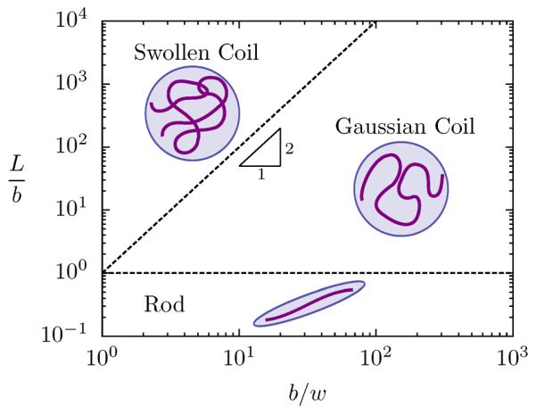
Summary of the classical scaling arguments for a real semiflexible chain in dilute suspension. Three regimes are predicted based on the interplay between the contour length (L), the chain stiffness (l_p) and the chain width (w). Very short chains (L ⪡ l_p) are rod-like and long “thin” chains are nearly Gaussian (L ⪢ l_p and L ⪡ l_T). Long chains (L ⪢ l_T) are swollen coils.

Consider the case of a chain with a constant b/w, which would be a vertical trajectory in Fig. 1. When L ⪡ l_p, the chain is short and rigid like a rod and the size of the polymer — which we represent with the end-to-end distance R without a loss of generality — scales linearly with the contour length

$$R~L$$ (15)

When the chain is much longer than the persistence length L ⪢ l_p, the thermal fluctuations of the chain overwhelm the bending energy and the shape becomes a flexible coil. However, if the polymer is short enough, there are few intrachain interactions and the molecule experiences negligible excluded volume interactions giving

$$R~{\left(\mathit{bL}\right)}^{1∕2}$$ (16)

which is the familiar random walk scaling.

For any real (self-avoiding) chain, the magnitude of the total excluded volume interactions increases as the contour length increases. When the excluded volume energy is on the order of k_BT, a second transition occurs from a Gaussian to a swollen coil. The size of a swollen coil is given by the radius⁵

$$R~b{\left(\frac{w}{b}\right)}^{2{\nu }_F-1}{\left(\frac{L}{b}\right)}^{{\nu }_F}$$ (17)

where ν_F = 0.587597(7)⁴¹ is the modern value of the Flory exponent.

Just as the rod-to-coil transition is characterized by the persistence length, the Gaussian-to-swollen coil transition is given by the contour length contained in a thermal blob

$$l_T\equiv c\frac{b^3}{w^2}$$ (18)

with c given as a scaling constant. Normalizing Eq. 18 by the Kuhn length b reveals the dependence of l_T on the monomer anisotropy b/w, which is the ratio of the “stiffness” to the “thickness” of the chain.^2,22,58 Thus when L ⪡ l_T, the chain is too stiff and thin to swell and the chain scales like Eq. 16, whereas when L ⪢ l_T the chain experiences sufficient excluded volume interactions to scale like Eq. 17.

An equivalent picture to the thermal blob (to within a constant factor) that often appears in the theoretical polymer physics literature^59,60 is the excluded volume parameter^5,58

$$z\equiv {\left(\frac{3}{2\pi }\right)}^{3∕2}\frac{w}{b}{\left(\frac{L}{b}\right)}^{1∕2}$$ (19)

with the conventional prefactor. Here z ≈ 1 signifies the transition point between Gaussian and swollen behavior.

3.2 Model Parameterization

Since we are interested in moving beyond scaling theory and making quantitative predictions of the properties of single-stranded and double-stranded DNA, we need to parameterize the DWLC model to experimental data. In particular, we need values of the persistence length, l_p, (or equivalently the Kuhn length), the effective width, w, and the bond length, a, in order to specify equilibrium properties. To specify dynamic properties, we also need the hydrodynamic diameter, d, but we defer this discussion until Sec. 3.4.

As polyelectrolytes, the magnitude of the persistence length and the effective width of single-and double-stranded DNA depend on the ionic strength.⁶¹ The effect of ionic strength, I, on the persistence length of double-stranded DNA has been examined by both experiments^6,26,62–66 and theory.^67–69 While some disagreements remain regarding the effects of electrostatics on l_p at very low values of the ionic strength, empirical results and theories generally agree for large values of I.⁶¹ Perhaps due to lesser prominence or greater measurement difficulty, there seems to be little controversy surrounding the magnitude and ionic strength dependence of the effective width of dsDNA. More than three decades ago, Stigter used the calculation of the second virial coefficient of a stiff, charged rod to predict the width,^61,70 and it has been subsequently corroborated by DNA knotting experiments.⁷¹

Figure 2 summarizes the ionic-strength dependence of dsDNA of both the Kuhn length (using an empirical relation from Dobrynin^61,69) and the effective width (using Stigter's theory⁷⁰). As has been pointed out before,⁶¹ both b and w rise as the ionic strength decreases, making the chain stiffer. However, above 10 mM the Kuhn length changes much less quickly than the effective width, meaning that the monomer anisotropy ratio drops rapidly as the ionic strength decreases. Therefore as b/w falls with decreasing ionic strength, the Kuhn monomers of dsDNA become less anisotropic and the chain becomes more flexible in the long chain limit. The effect on the scaling behavior of finite length chains is non-trivial however, since there is a competition between decreasing the anisotropy of the Kuhn monomers and decreasing their number. For instance, near 10 mM the monomer anisotropy ratio for dsDNA falls below 10, but the number of Kuhn monomers in T4-DNA remains high (≈ 400). However, by 0.1 mM the anisotropy ratio drops below 3, but the number of Kuhn lengths is reduced to approximately 100.

Figure 2.

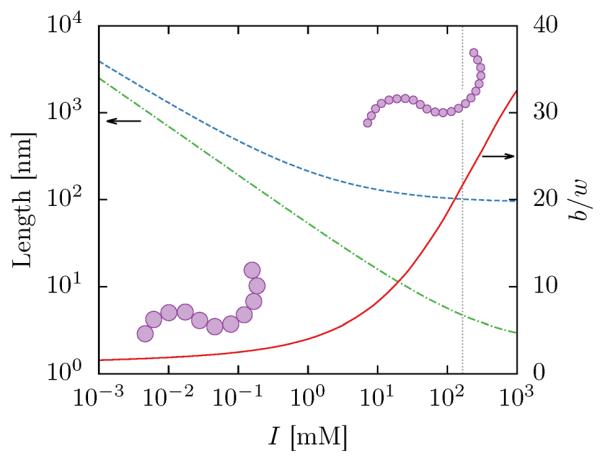
Ionic strength dependence of the Kuhn length (dashed blue line) and the effective width (dot-dashed green line) and the monomer anisotropy (solid red line) for dsDNA. The vertical gray dotted line indicates an ionic strength of 165 mM (≈ 5× TBE).⁶¹ The schematic illustrates two chains with similar b but different w, demonstrating the decrease in monomer anisotropy as the effective width increases more rapidly than the Kuhn length.

To simplify the model, we limit our scope to high ionic strengths where strong electrostatic screening marginalizes the effect of the electrostatics.⁶¹ This assumption allows us to neglect electrostatic potentials in our model and use constant values of b and w. When necessary, we assume an ionic strength of 165 mM, which corresponds to 5× TBE⁶¹ and is marked with a gray vertical line in Figure 2. Assuming these buffer conditions gives b = 106 nm, which has become the consensus Kuhn length of dsDNA,⁶ and w = 4.6 nm, the value obtained from Stigter's theory.^22,61,70

Unlike dsDNA, even a simple measure of the persistence length of ssDNA in a high ionic strength buffer remains controversial. A survey of the recent literature reveals studies done by mechanical stretching,^26,72 fluorescence recovery after photobleaching,⁷³ fluorescence resonance energy transfer^29,30 and small-angle x-ray scattering^28,29 that yield values of the bare persistence length (at infinite ionic strength) between 0.6 and 1.3 nm. It seems likely that base-base interactions are responsible for the disagreement and recent work on non-interacting ssDNA sequences^28,29 gives a consistent value of 1.5 nm at the aforementioned ionic strength of 165 mM.

Assuming rod-like interactions for the effective width, which forms the foundation of Stigter's theory, appears to be inappropriate for ssDNA. Some experimental work suggests that for ssDNA, w is nearly independent of ionic strength⁷² and that its value is approximately equal to the bare persistence length of the chain.²⁸ Accordingly, we adopt a value of 0.65 nm,²⁸ which conveniently also appears to be the approximate rise of a single base of ssDNA.⁷⁴

Finally, because we have a discrete model, we must specify a bond length a. Since dsDNA is well-described by a continuous model, the choice of a is somewhat arbitrary so long as a ⪡ b, much like a time step in numerical integration schemes. In this case we choose a = d, which is the smallest length scale in the model. This is commonly called the touching-bead model^48,75 and is also advantageous for the calculation of the diffusivity. In addition to the far-field approximation mentioned in Sec. 2.3, the DWLC estimation of the Kirkwood diffusivity also introduces discretization errors into the diffusivity; accurate hydrodynamic interactions require the collective action of many Stokeslets, which in turn requires a large number of beads. The touching-bead model provides adequate resolution of the chain to satisfy this condition and has the additional benefit of circumventing any artifacts in the hydrodynamics due to a variable bond length.

The choice of a for ssDNA is less clear than for dsDNA, since both continuous and discrete models have been used with some success for ssDNA.^20,26–28 The Kuhn length (≈ 3 nm) provides the upper bound for a, and it is sufficiently small that the lower bound is given is given by the chemical monomer size (≈ 0.6 nm). As discussed in Sec. 2.1, a choice of a > w is problematic, so for convenience we set a = w. For the reader's convenience, the model parameters are summarized in Table 1.

Table 1.

Parameters of the discrete wormlike chain for double- and single-stranded DNA in a high ionic strength buffer (e.g.≈ 5× TBE). All of the parameters are lengths expressed in nm. Note that while our model parameters are defined in some cases to sub-angstrom precision, this does not reflect the true experimental accuracy of these parameters.

Parameter	Symbol	ssDNA	dsDNA
Kuhn length	b	3.0	106
effective width	w	0.65	4.6
hydrodynamic diameter, bond length	d, a	0.65	2.9

PERM calculations were performed with the parameters in Table 1 to verify the model. Results for the radius of gyration are shown in Fig. 3 where they are compared to experimental values of the radius of gyration of undyed dsDNA obtained by light or neutron scattering.^9,76–86 There is excellent agreement between the experimental data and the PERM results. However, given that there are two degrees of freedom (l_p and w) to fit the experimental data, the good agreement between theory and experiment is expected.

Figure 3.

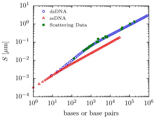
PERM data for the radius of gyration of ssDNA (open red triangles) and dsDNA (open blue circles) compared to experimental data for dsDNA from light and neutron scattering (filled green squares).^9,76–86 The experimental data were obtained from many different references, at varying ionic strength (all ≥ 100 mM), with varying information about the molecular weight. To obtain a consistent value, the molecular weight of dsDNA was assumed to obey the relation 660 Da = 0.34 nm = 1 bp. Single stranded DNA was assumed to follow 1 base = 0.65 nm.

Even with the excellent agreement, the effective width w remains a somewhat uncertain parameter. Eq. 17 predicts that S ~ w^0.175, demonstrating that the radius of gyration is not very sensitive to the effective width. This means that S is not particularly useful at evaluating the ability of the model to capture the correct strength of the excluded volume. Compounding this fact, it appears to be difficult to collect accurate data for the radius of gyration at large L.

Thus, despite our best efforts to pick accurate model parameters, our choice is certainly a possible point of contention. Indeed, our parameters give a monomer anisotropy b/w ≈ 23 for dsDNA, whereas others have estimated an anisotropy as high as 66.² Implicit in this disagreement, and further muddying the waters, is the role of intercalating dyes mentioned in the introduction. Both the persistence length and effective width are clearly affected by the presence of dyes,¹⁴ but consistent measurements of their effects have not been possible to date.^15,16 Consequently, we have omitted data for dyed dsDNA from Fig. 3, since reported radius of gyration measurements are inferred from diffusivity measurements, which are not static measures. In fact, in Sec. 3.4, our results suggest that this introduces a source of systematic error since the chain has not yet reached the long-chain limit. Therefore, until more data regarding the effective width and a resolution of the dye-dependence of both l_p and w becomes available, the parameters for dyed dsDNA will remain somewhat uncertain.

Finally, in addition to the PERM calculations, we also found it useful to employ renormalization group theory (RG) results by Chen and Noolandi⁶⁰ for the end-to-end distance and radius of gyration. In contrast to the Monte Carlo results, the RG theory gives R and S only, but the metrics are available as a function of molecular weight to practically unlimited contour lengths. Note that since the RG calculations employ a continuous model, the excluded volume strength in the RG theory must be re-parameterized to agree with the experimental and PERM data (see online supporting information).

3.3 Equilibrium Properties of DNA

Given that we have a parameterized model for single-stranded and double-stranded DNA, we are prepared to move beyond the insights of scaling theory and examine detailed quantitative calculations of dilute solution equilibrium properties. To begin, we examine the value of the apparent power-law exponent of the end-to-end distance

$$\nu \equiv \frac{\mathrm{d}\ln R}{\mathrm{d}\ln L}$$ (20)

as a function of molecular weight. While this can be done with PERM, the end-to-end distance is also available from the RG theory of Chen and Noolandi,⁶⁰ which we parameterize to match the PERM data (see online supporting information). The RG theory is only available for only a few equilibrium properties, but it provides results over a much larger range of contour lengths than one can obtain with PERM. In addition, the RG theory has no sampling error and gives a much smoother value of ν.

Fig. 4 shows the RG theory results for the power-law exponent, ν, as a function of L/b. As a reference, results are shown for several different values of the monomer anisotropy, w/b, not just ssDNA and dsDNA. At first glance, nothing appears spectacular about the plot; it agrees very well with scaling theory. For instance, consider the curve corresponding to w/b = 3.16 × 10⁻³. When L/b small, the chain is rod-like and around L/b = 1, the exponent falls rapidly, approaching ν = 0.5. As L/b increases, excluded volume gradually dominates and the exponent approaches 0.588. Furthermore, the dependence on w/b of the transition from Gaussian to swollen coils also agrees with scaling theory. For w/b near 1 (ssDNA), the chain shows effectively no Gaussian regime and the chain transitions from rod-like to swollen coil very quickly. Whereas, when w/b is near 0 (w/b = 3.16 × 10⁻⁴) a large Gaussian regime appears and the transition to a swollen coil is delayed.

Figure 4.

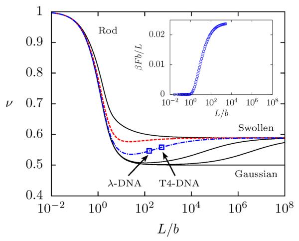
Power-law exponent of the end-to-end distance of a semiflexible chain with excluded volume as calculated by results from renormalization group theory.⁶⁰ As outlined in Sec. 3.1, ν = 1 corresponds to rod-like behavior, ν = 0.5 to a Gaussian chain and ν = 0.588 to a swollen chain. Results are shown for five different values of w/b (from top to bottom): 1.0, 0.217 (ssDNA), 0.043 (dsDNA), 3.16 × 10⁻³, 3.16 × 10⁻⁴ and 0 (no excluded volume). (Inset) PERM results for the excess free energy per Kuhn length due to excluded volume interactions in a dilute solution of dsDNA.

In addition, Fig. 4 supports the contemporary interpretation of ssDNA as a flexible chain. The scaling exponent transitions practically immediately to an excluded volume chain and by about 500 bases the exponent is 0.58 — within 1% of Flory scaling. (It should be noted that the RG calculations limit to a value of ν = 0.5886,⁶⁰ slightly larger than the value of ν_F reported by Clisby.⁴¹)

However, the asymptotic and continuous transitions between regimes in Fig. 4 are unknown from scaling theory, and these transitions have a major consequence on the implications of scaling theory for dsDNA. As the RG calculations show, double-stranded DNA is an intermediate case, with a monomer anisotropy w/b ≈ 0.04 and is therefore neither thin nor stiff enough to exhibit a true Gaussian coil regime. In fact, the minimum exponent shown in Fig. 4 is ν = 0.535 at 8.3 kilobase pairs (kbp), which is about halfway between 0.5 and ν_F. Additionally, the transition of dsDNA to a completely flexible coil is exceptionally broad.¹⁷ At 48.5 kbp (λ-DNA), the exponent (ν = 0.546) is only slightly higher than the minimum; by the time the chain reaches 1 megabase pair (Mbp), the exponent has reached 0.572, which is within 3% of ν_F.

Thus, the continuous and asymptotic nature of the transitions obfuscates the scaling theory picture of dsDNA. Accordingly, Fig. 4 provides an excellent explanation for the confusion surrounding the scaling of dsDNA. That is, for most practical purposes, kbp-length dsDNA is neither “ideal” or “real”, but an intermediate case.

Given that the transitions are smooth, one would expect excluded volume effects to play a non-negligible role for dsDNA at intermediate contour lengths, well before the flexible chain limit is reached. This is indeed the case. One informative way to see this is through the excess free energy per Kuhn monomer due to excluded volume interactions shown in the inset of Fig. 4 as a function of contour length. Observe that the excluded volume interactions begin to “turn on” very early, near L/b ≈ 1, which explains why dsDNA never truly approaches Gaussian scaling. The free energy curve then consumes another three decades in L/b before it nears the asymptotic limit, which further accounts for the broad transition to Flory scaling.

Another consequence of the gradual ramp-up of excluded volume interactions manifests itself through the form factor, which is particularly useful for studying the scaling behavior. The form factor is not only directly available from light scattering experiments,⁵ but as the Fourier-transform of the pair-correlation function, it provides information about a variety of length scales of a given polymer as a function of the wave vector. In particular, we are interested in the so-called fractal regime qS ⪢ 1 where q is the magnitude of the wave vector and S is the radius of gyration. This regime provides information related to the chain statistics inside the coil, which can reveal details about stiffness and self-avoiding behavior.

The expression for the form factor of a Gaussian chain is the well-known Debye equation

$$P\left(q\right)=\frac{2}{{\left(\mathit{qS}\right)}^4}\left[\exp \right(-q^2{S}^2)-1+q^2{S}^2]$$ (21)

Since a wormlike chain includes small length scale effects that are unaccounted for by the Gaussian chain model, the Debye expression is not always valid in the fractal regime. There is a (somewhat complicated) analytical expression for the form factor of an ideal wormlike chain (see online supporting information as well as Spakowitz and Wang⁸⁷). The basic result mirrors scaling theory; length scales where ql_p ⪡ 1 behave like coils and agree with Eq. 21, whereas length scales where ql_p ⪢ 1 behave rod-like and disagree with Eq. 21.

The problem becomes more complicated when we include the effect of excluded volume. Although, a closed-form expression for the form factor of a wormlike chain with excluded volume is not available, it can be computed numerically.^17,18,88 Additionally, Sharp and Bloomfield⁸⁹ have provided a semi-empirical relation (for additional details see online supporting information). However, scaling again helps us interpret the anticipated results. When z ⪡ 1 coils should scale like P(q) ~ q^−1/2, which agrees with the Debye equation, and when z ⪢ 1 the form factor should scale like q^−1/ν_F.

Fig. 5 shows the form factor of several different lengths of dsDNA in the fractal regime using PERM. In this region in particular, long chains such as λ-DNA show a deviation from Eq. 21 due to excluded volume effects. This can be seen by the gradual transition from a slope of −1/2 for short chains (which agrees well with the Debye expression) to a slope of −1/ν_F for long chains.

Figure 5.

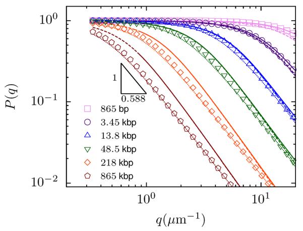
Form factor of dsDNA for ql_p < 1 for various contour lengths (from left to right): 865 kbp, 218 kbp, 48.5 kbp (λ), 13.8 kbp, 3.45 kbp, 865 bp. Symbols correspond to PERM calculations (with excluded volume), dashed lines to Eq. 21 and dotted lines to a semi-empirical expression by Sharp and Bloomfield.⁸⁹ Solid lines correspond to the form factor of an ideal wormlike chain with the same stiffness⁸⁷ (see online supporting information).

The excluded volume dependence of the form factor is of particular importance when extracting the radius of gyration or persistence length from light scattering measurements.^8,9,62,89,90 This is supported by Fig. 5, which shows that a systematic bias in the fitting parameters (i.e. the radius of gyration) is present if Eq. 21 is used to fit the PERM data for long chains. We speculate this principle provides an explanation for the contradiction between the radius of gyration extracted from classic light scattering studies on T7 DNA (40 kbp),⁸ which showed excluded volume effects, and recent fluorescent correlation spectroscopy measurements of chains up to 97 kbp,⁷ which did not. Accordingly, we conclude that one must resort to either simulations or the semi-empirical relation of Sharp and Bloomfield to accurately estimate the size of long dsDNA.

Thus far we have discussed two principles that emerge from a quantitative evaluation of the equilibrium properties of DNA (and semiflexible chains in general). Namely, transitions are smooth and asymptotic and excluded volume effects are important at length scales well below the flexible limit. Additionally, simulation results show that different size metrics have quantitatively different transitions. Since scaling theory is unable to predict such transitions, this has been underappreciated in the literature. In fact, when combined with smooth and broad transitions, metric-dependent transitions make it very difficult (if not impossible) to define an objective measure of when a wormlike chain like DNA is “in a regime.”

To see this, consider Fig. 6 which depicts the scaling exponent ν for the size metrics S and R from both PERM and RG calculations as well as X, which is available from PERM alone. Due to high-frequency fluctuations in the PERM data, the derivative ν was determined by a Savitsky-Golay filter with second-order polynomials. Even with the filter, some low-frequency noise still exists in the data, causing fluctuations at large molecular weights. Nevertheless, the PERM results for the radius of gyration and end-to-end distance agree very well with the RG theory calculations until very small L, which is caused by the discretization of the DWLC model.

Figure 6.

PERM calculations of dsDNA for the value of the exponent ν in R ~ L^ν (blue circles), S ~ L^ν (red triangles) and X ~ L^ν (green diamonds) for dsDNA (w/b = 0.0434) ~ and RG calcula tions for ν for R (blue dashed line) and for S (red solid line). The dashed gray lines correspond to the values of ν = 0.5 (Gaussian) and ν = 0.5876 (swollen).

Fig. 6 clearly shows that each metric has a different minimum and a different approach to the long-chain limit. For instance, it appears that the end-to-end distance has the deepest minimum and the longest climb to the asymptotic limit whereas the mean span has a very shallow minimum. Consequently, with finite contour lengths, any computation or measurement is going to exhibit metric dependent behavior. In other words, measurements with the same molecular weight of dsDNA with different metrics will result in different scaling exponents. Furthermore, it appears for some molecular weights, that the measured scaling exponent ν may be more sensitive to the size metric than to the contour length.

The dependence of the scaling exponent on the size metric also illuminates the concept of the thermal blob. Briefly introduced in Sec. 3.1, the thermal blob can be understood as a renormalized monomer in a flexible, self-avoiding chain. In other words, a very long, flexible chain can be viewed as a self-avoiding walk of thermal blobs⁵

$$\frac{\Xi }{{\xi }_{\mathrm{T}}}~{\left(\frac{L}{l_{\mathrm{T}}}\right)}^{{\nu }_{\mathrm{F}}}$$ (22)

where Ξ is some size metric (e.g. radius of gyration), L is the total contour length and ξ_T is the size of a blob composed of a subsection, l_T, of the contour length of the original chain. Therefore to be truly flexible and self-avoiding, the contour length of a chain must be much greater than the blob length and its size must be much greater than the blob size.

Since the thermal blob length is a scaling parameter, it is useful as a qualitative measure only, and consequently, one should not expect a single value of l_T to provide a precise value of the minimum length-scale for excluded volume interactions. This enters explicitly in the definition of the thermal blob length l_T in Eq. 18 where the constant c was left undefined. Nevertheless, there are several definitions of c which are commonly encountered in the literature and we find it useful in Table 2 to make a comparison of the contour length and size of the resulting thermal blob obtained using these definitions.

Table 2.

Thermal blob length l_T and size ξ_T of ssDNA and dsDNA determined using different choices of scaling constant c and different size metrics. The thermal blob length and size for the F = k_BT case were computed using PERM calculations for the excess free energy and the various size metrics respectively.

	l T
	ssDNA	dsDNA
c = 1	64 bases	166 kbp
z = 1	587 bases	1520 kbp
F = kBT	45 bases	16.8 kbp

	ξT (F = kBT)
	ssDNA	dsDNA
End-to-End Distance	10.2 nm	825 nm
Radius of Gyration	3.9 nm	332 nm
Mean Span	7.3 nm	678 nm

As a first estimate, one may simply set c = 1, which gives l_T = 64 bases for ssDNA and l_T = 166 kbp for dsDNA. One may also set the excluded volume parameter z equal to one, which leads to c = (2π/3)³ and consequently l_T = 587 bases for ssDNA and l_T = 1.52 Mbp for dsDNA. A more rigorous definition sets the thermal blob length to be the contour length of a chain where the excess free energy from excluded volume is equal to k_BT.^5,91 Since PERM directly computes the excess free energy, this length is immediately available and yields c = 0.102 for dsDNA (16.8 kbp) and c = 0.458 for ssDNA (45 bases).

Even for a fixed value of c, the thermal blob size, ξ_T, also depends on the size metric. Table 2 shows one such example using F = k_BT to pick c. Here, with a fixed contour length of l_T = 16.8 kbp, the radius of gyration of a thermal blob of dsDNA is 332 nm, but the end-to-end distance is 825 nm. Similarly, for l_T = 45 bases, the radius of gyration of a thermal blob of ssDNA is 3.9 nm, but the end-to-end distance is 10.2 nm.

While it is not surprising that l_T and ξ_T vary with the choice of c and size metric, the magnitude of the variation that is represented in Table 2 is somewhat startling. Given reasonable but different choices of the constant c in Eq. 18, we find that the thermal blob length can vary by nearly two orders of magnitude and encompasses much of the range of molecular weights available for experiments. The large variation in the thermal blob lengths in Table 2 further emphasizes their qualitative nature and cautions that these values should only be considered rough order of magnitude estimates of the length-scale where excluded volume and bending effects are approximately equal. Finally, this variation suggests that a direct computation of “how many thermal blobs are in a chain” is not meaningful without a specific definition of c. For instance, using the various definitions of c found in Table 2, λ-DNA can be reported to have 2.9 (F = k_BT), 0.29 (c = 1), or 0.032 (z = 1) thermal blobs. In contrast to these estimates, when prefactors and transitions are fully resolved, we unambiguously show in Fig. 4 and Fig. 6 that λ-DNA is in the middle of a transition from ideal to Flory scaling.

3.4 Dynamic Properties of DNA

To this point, the discussion has focused on the equilibrium properties of DNA and the role of excluded volume as a wormlike chain approaches the flexible chain limit. However, the near-equilibrium diffusion coefficient and other dynamic properties also play a prominent role in the use of dsDNA as a model polymer. The effects of solvent mediated interactions between distal chain segments, called hydrodynamic interactions (HI), are central to dilute solution DNA dynamics. Hydrodynamic interactions are in many ways the dynamic counterpart to excluded volume interactions, and their inclusion introduces a degree of freedom through the hydrodynamic diameter d.

Despite some similarities, the hydrodynamic diameter is not in general equal to the effective width w, since chain friction and excluded volume arise from distinct physical phenomena. In principle, the hydrodynamic diameter corresponds to the surface of shear of the molecule and is an intrinsic property of a polymer chain. However, in our case we have employed a far-field approximation (Eq. 13) that neglects near-field lubrication forces, rendering the hydrodynamic diameter a phenomenological parameter.

With the addition of a degree of freedom for the hydrodynamic interactions, the landscape of possible types of diffusive behavior for a wormlike chain becomes complicated.⁹² The diffusion coefficient depends not only on configurational properties (including excluded volume), but also on the strength of the HI. In other words, there is not a simple one-to-one correspondence between configuration and diffusive behavior (even for very flexible chains). The literature identifies at least three classes of behavior that a wormlike chain can exhibit, which are shown in Fig. 7.

Figure 7.

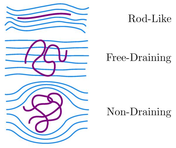
Schematic of diffusive behaviors of wormlike chains. Rod-like diffusion dominates for very short, stiff chains. Polymer coils can exhibit either free-draining (weak HI) or non-draining (strong HI) behavior. Partial draining behavior is also possible for chains with relatively open structures. In this case, the polymer conformation is not sufficient to describe the diffusive behavior of the chain since the strength of the HI (i.e. the hydrodynamic radius) can vary independently.

For very short and stiff conformations with HI, the chain exhibits rod-like diffusion^47,51,93

$$D_{\text{rod}}=\frac{k_{B}T}{3\pi \eta L}\left[\ln \right(L∕d)+\gamma ]$$ (23)

where η is the solvent viscosity and γ is in general a function of L/d, and equals 2ln2 – 1 in the slender-body limit. For more flexible chains, one can distinguish between the case where HI is weak (free-draining) and the case where HI is strong (non-draining).⁹⁴ As indicated in Fig. 7, a free-draining coil experiences no hydrodynamic screening and interacts fully with the solvent giving the Rouse diffusion coefficient⁵¹

$$D_{\text{Rouse}}=\frac{k_{B}T}{6\pi \eta L}$$ (24)

The non-draining coil has significant HI and is impermeable to solvent flow. For a flexible chain with no excluded volume interactions, the diffusion coefficient was derived by Zimm^51,94

$$D_{\text{Zimm}}=\frac{8}{3\sqrt{6{\pi }^3}}\frac{k_{B}T}{\eta \sqrt{\mathit{Lb}}}$$ (25)

and gives a diffusion coefficient that is inversely proportional to the coil size.

While it is clear that a wormlike polymer may exhibit any one of these classes of behavior, a comprehensive qualitative description of the problem for wormlike chains remains elusive. Indeed the inclusion of the effects of flexibility, excluded volume and hydrodynamic interactions has proven to be an exceedingly difficult task^{12,47,92,95,96} and accordingly, no complete analytical theory exists to date. However, several important pieces have been developed since the work on flexible polymers by Zimm,⁹⁴ some of which are noteworthy.

First, Oono and Kohmoto^51,95 used a dynamic renormalization group theory to find the diffusivity of a flexible polymer chain with both EV and HI. In agreement with the result by Zimm, the diffusivity

$$D_{\text{Oono}}=\frac{1}{12.067}\frac{k_{B}T}{\eta S}$$ (26)

suggests that the long-chain limit is characterized by non-draining coils where the dynamics are governed by conformational effects only (the hydrodynamic diameter is conspicuously absent).

However, further work by Douglas and Freed⁹² displays a complicated picture for finite-length chains where excluded volume effects (which swell the coil) act in competition with hydrodynamic interactions which decay with decreasing chain density. This competition can lead to partial-draining, an intermediate state between the free-draining and non-draining limits pictured in Fig. 7, where the configurational properties of the chain are insufficient to completely describe the diffusivity. Thus even very long (but finite) chains may not obey Eq. 26, but will include a dependence on the hydrodynamic diameter.

In an orthogonal attempt, Yamakawa and Fujii⁴⁷ computed the diffusivity of an ideal wormlike chain, which accounts for chain stiffness and HI, but neglected the effects of excluded volume (see supporting information online). The wormlike chain diffusivity shows a gradual crossover from rod-like behavior (Eq. 23) to Zimm diffusion (Eq. 25) as the contour length increases, which in turn means a gradual decrease in the effect of the hydrodynamic diameter. Given that our DWLC model incorporates all of the effects listed above, we anticipate that the diffusion of DNA will include effects from each of these previous works.

To correctly capture the dynamics, we need an accurate estimate for the hydrodynamic radius d of ssDNA and dsDNA. Literature values for the hydrodynamic diameter of dsDNA have been obtained by a variety of experimental methods and typical values vary between 2 to 3 nm.^{11,47,76–80,82–85,97–107} Less is known about the hydrodynamic radius of ssDNA. The diffusivity of short ssDNA chains can be sequence dependent due to base-pair interactions thus requiring thermal and chemical denaturing agents,⁷³ which makes generic diffusivity studies difficult.¹ Due to a lack of data therefore, the hydrodynamic radius is uncertain, and we simply assume that d = w.

To get a more precise value of d for dsDNA, Fig. 8 shows a meta-analysis of several measurements of the diffusivity of dsDNA in the literature.^{11,76–80,82–85,97–104} Here, the Kirkwood diffusivity for dsDNA is plotted alongside the experimental data as a function of molecular weight, which is rescaled by the Zimm diffusion given in Eq. 25. Note that Eq. 25 is not defined in terms of the radius of gyration, S, of the polymer, but rather in terms of the contour length, L, and Kuhn length, b. This allows an unambiguous comparison to a larger experimental data set since there is only a small overlap between the sources of experimental data for the diffusivity (Fig. 8) and the radius of gyration (Fig. 3). The hydrodynamic radius is extracted by comparing the experimental data to the theory of Yamakawa and Fujii⁴⁷ for the diffusion of a wormlike chain without excluded volume. This is justified since the diffusivity is most sensitive to the hydrodynamic radius at low L where hydrodynamic screening and excluded volume interactions are negligible. As seen in Fig. 8, the value of 2.9 nm (which agrees with an analysis by Lu et al.¹⁰⁶) fits the low molecular weight data exceptionally well.

Figure 8.

Parameterization of the hydrodynamic diameter for the DWLC. (A) Curves (black, blue, red) show the relative diffusivity of a CWLC without excluded volume⁴⁷ at different values of b/d. The touching bead DWLC model (symbols) shows excellent agreement with the CWLC chain (curves). (B) Experimental data for the diffusivity from dynamic light scattering (filled green triangles),^{82–84,97–101} sedimentation (filled green circles),^{76–80,85,102,103} and single molecule methods (open green triangles).^11,104 The dsDNA data fits the DWLC simulation (now with excluded volume interactions) for b/d = 36 or d = 2.9 nm. Notice that since the diffusivity is scaled by the Zimm diffusion (ideal chain diffusion), the asymptotic value does not approach 1. Additionally, it appears that the single molecule data give poorer agreement with the simulation data, presumably due to the impact of intercalating dyes.

Fig. 8(B) also shows that at large contour length, the PERM diffusivity calculations give excellent agreement with values of the diffusion obtained from dynamic light scattering (DLS) and sedimentation experiments. The agreement with the experimental data at low molecular weight is expected, since it was used to obtain the hydrodynamic radius. However, the agreement with the DLS and sedimentation data persists for large molecular weights, when excluded volume effects cause the chain to swell. This suggests that the both the size and degree of hydrodynamic screening of the dsDNA coil is well described by the DWLC model.

In contrast, the DWLC model does not agree well with single molecule diffusivity measurements from fluorescence microscopy,^11,104 which we hypothesize is due to the presence of intercalating dyes. It is unclear how the width, persistence length and hydrodynamic radius of DNA change with intercalating dyes,^15,16 making it difficult to computationally replicate their effect on diffusivity. Since the contour length of λ-DNA is observed to increase from 16.3 μm to about 21 μm, a common supposition is that all properties increase by a constant factor, leaving the ratios between properties constant. This proposition is easily tested by our model, and assuming an increase of 28%, we find that the change in diffusivity is insufficient to explain the disagreement (see supporting information online). Instead, we conclude that in addition to changing the contour length, fluorescent dyes are likely to alter the ratios b/w and d/w. Indeed, this appears reasonable since the positively charged dyes lead to a decrease in the effective charge of the DNA,¹⁰⁸ which may decrease the effective width.

Moving forward, we would like to examine the behavior of ssDNA and dsDNA as the diffusivity approaches the long chain limit. Notice that if we introduce the definition of the chain hydrodynamic radius

$$R_{\mathrm{H}}\equiv \frac{k_{B}T}{6\pi \eta D}$$ (27)

The ratio of the radius of gyration to the hydrodynamic radius becomes⁹⁵

$$\frac{S}{R_{\mathrm{H}}}=1.562\frac{D}{D_{\text{Oono}}}$$ (28)

In the long-chain limit, D → D_Oono and the ratio is predicted to converge to a universal value of 1.562.⁹⁵

Fig. 9(A) shows the ratio S/R_H as a function of molecular weight. As expected, both curves appear to approach a constant value in the limit that L → ∞, but the value appears slightly larger than predicted by the renormalization group theory. (A least squares fit to the ssDNA data for L > 2000 bases gives S/R_H = 1.58902(2).) For ssDNA, the story is much the same as it was for static properties; within 100 bases, the diffusion appears to have reached its long-chain limit. Also similar to the static size measures, it takes an exceptionally long dsDNA chain to reach the flexible coil limit. According to Fig. 9(A), dsDNA is within about 1% of the value predicted by Oono and Kohmoto⁹⁵ by the terminal molecular weight of 865 kbp.

Figure 9.

(A) PERM results for the ratio of the radius of gyration S to the hydrodynamic radius R_H as a function of the molecular weight for both ssDNA (open red triangles) and dsDNA (open blue circles). λ-DNA and T4-DNA are shown for reference (arrow, open orange squares). The horizontal dashed line corresponds to S/R_H = 1.562. (B) The diffusion coefficient from PERM, rescaled by Eq. 25, as a function of the number of base pairs of DNA. Double-stranded DNA is shown to transition from rod-like behavior (green dashed line) to non-draining behavior (purple dotted line) over several orders of magnitude in molecular weight. The diffusion coefficient without excluded volume (closed blue circles) is shown for reference.

The claim that dsDNA converges very slowly to its long-chain value is at odds with earlier experimental work which asserted that λ-DNA is fully swollen and non-draining.^11,104 However, the evidence for non-draining coils is based upon the measured scaling exponent (ν = 0.61), which appears to be relatively unresponsive to the draining behavior of dsDNA (see supporting information online). Experimental work by Schroeder et al.^10,109 made more sensitive measures of the hydrodynamic behavior of dsDNA by studying the phenomena of conformation hysteresis. Schroeder et al. found that significant hydrodynamic effects were observed for chains near 1.3 Mbp, and that it took a nearly 3 Mbp polymer to achieve the sought-after hysteresis. While these experiments did not search for the onset of HI interactions per se, the effects of HI are observed in chains with molecular weights within an order of magnitude of those predicted by our calculations. Subsequently, their observations support our conclusion that extremely long chains are needed to achieve non-draining behavior.

The slow convergence to non-draining behavior also has practical implications for the measurement of the radius of gyration in fluorescence microscopy experiments. It is common practice to use fluorescence microscopy measurements of the diffusivity to estimate the radius of gyration by assuming that the D/D_Oono = 1 in Eq. 28.^11,104 As shown by Fig. 9(A) there is always some systematic bias made by this inference. However, the bias decreases as molecular weight increases making the assumption justified at very large molecular weights. Assuming that the constant 1.562 is exact (which is questionable), this method underestimates the radius of gyration of λ-DNA by about 9%.

The extremely large molecular weights required to reach the non-draining limit also bring to mind the previous discussion surrounding partial draining. To further understand the partial draining of dsDNA, consider Fig. 9(B), which shows the normalized Kirkwood diffusivity as a function of molecular weight. Here the diffusivity is shown to cross over from rod-like diffusion (Eq. 23) at low molecular weights to non-draining diffusion (Eq. 26) at large molecular weights. According to Fig. 9(B), dsDNA less than a few hundred base pairs is well approximated by rod-like diffusion (to within a constant factor). This seems reasonable, given that a chain of 156 bp is about one persistence length. As the contour length increases, the diffusivity is observed to asymptotically approach the non-draining limit. Consistent with the previous analysis, this asymptotic approach is slow, and λ and T4 DNA give diffusivities that are respectively 9% and 4% greater than the asymptotic limit. We conclude therefore, that kilobase-pair length dsDNA is partially draining.

While partial draining has been a subject of discussion since at least 1979 (couched in terms of dynamic scaling³), it has become a topic of recent interest in both free solution^12,110 and confinement.^13,45,111 Interestingly, Mansfield and Douglas¹² suggest that transport properties are especially slow to converge to their long-chain values. Their work, which employs several different polymer models, suggests that a slow transition to non-draining behavior is not unique to DNA. This trend is also seen in recent work by Dai et al.¹³ on the diffusion of DNA in slits, which posits that the local pair correlation function of a polymer has a long-ranged impact on coil dynamics. Unfortunately, due to noise in the present data, it is difficult to tell whether or not the diffusion coefficient converges more slowly than the radius of gyration or other static measures.

4 Conclusion

Using a powerful Monte Carlo method, PERM, we have elucidated the long-chain behavior of both single-stranded and double-stranded DNA. Clearly, single-stranded DNA is much more flexible and several hundred bases are sufficient to guarantee both complete swelling and non-draining behavior. By contrast, double-stranded DNA is much slower to reach flexible-chain behavior. It appears that dsDNA much less than 1 Mbp should not be considered either completely swollen or fully non-draining. One immediate consequence of this result concerns the practice of inferring the radius of gyration of dsDNA from the diffusivity, which we find leads to a systematic bias (underestimation) in the measurement of the radius of gyration.

In addition, we find that shorter chains (e.g. λ-DNA), while not completely swollen, are nevertheless influenced by excluded volume and hydrodynamic interactions. This is complicated by the fact that the transitions between universal regimes are continuous and the approach is asymptotic and metric specific. Combined together, these observations suggest that it is inappropriate to consider λ-DNA as an “ideal” chain and neglect EV and HI. In some sense, λ-DNA is possibly the worst model polymer since it is clearly in a transition.

On the upside, even though the excluded volume and hydrodynamic interactions are significant, the languid transition towards universal behavior also indicates that the measured properties of dsDNA do not change rapidly as a function of contour length. In other words, practical estimates of the radius of gyration and diffusion coefficient are relatively unaffected by the change in scaling exponent as long as the change in molecular weight is not too great over the range of the estimate. Accordingly, Brownian dynamics studies that do not account for HI or EV explicitly, can in principle reproduce properties quantitatively by careful parameterization. However, such a parameterization will only be valid for a small range of contour lengths, and the properties obtained from subsequent simulations should be limited to this range. Nevertheless, prudence is warranted in interpreting such simulations, since the correct physics is not inherently incorporated.

Certainly, one troubling implication of our results concerns the lack of agreement with data from fluorescence microscopy experiments. We have attempted to justify this by the presence of fluorescent dyes, which alter the backbone of dsDNA. We believe that more work is needed to account for the disagreement and propose that the effects of intercalating dyes on dsDNA be studied in greater detail. In addition to this, we have not considered here the effect of changing ionic strength, which should be straightforward with minor modifications to the DWLC model.

In conclusion, we find it difficult to give a straightforward answer to the question: Is DNA a good model polymer? On the one hand, dsDNA continues to be widely used due to its extraordinarily useful experimental properties. Among others these include exquisite contour length selectivity, near monodisperse solutions, direct visualization techniques, ideal size relative to nanofabricated devices and end-attachment chemistry. On the other hand, if we narrow our scope to strictly universal behavior, megabase length chains appear to be necessary. Such long contour lengths give rise to experimental difficulties including chain cleavage and knotting, and at the present moment, it appears that such large chains are atypical in polymer dynamics experiments. Given this, we recommend caution in the interpretation of dynamic data obtained by shorter dsDNA.

References

- (1).Brockman C, Kim SJ, Schroeder CM. Soft Matter. 2011;7:8005–8012. doi: 10.1039/C1SM05297G. [DOI] [PMC free article] [PubMed] [Google Scholar]
- (2).Latinwo F, Schroeder CM. Soft Matter. 2011;7:7907–7913. doi: 10.1039/c1sm05298e. [DOI] [PMC free article] [PubMed] [Google Scholar]
- (3).de Gennes P-G. Scaling Concepts in Polymer Physics. Cornell University Press; 1979. [Google Scholar]
- (4).Freed KF. Renormalization Group Theory of Macromolecules. John Wiley & Sons, Inc.; 1987. [Google Scholar]
- (5).Rubinstein M, Colby R. Polymer Physics. Oxford University Press: 2003. [Google Scholar]
- (6).Bustamante C, Marko J, Siggia E, Smith S. Science. 1994;265:1599–1600. doi: 10.1126/science.8079175. [DOI] [PubMed] [Google Scholar]
- (7).Nepal M, Yaniv A, Shafran E, Krichevsky O. Phys. Rev. Lett. 2013;110:058102. doi: 10.1103/PhysRevLett.110.058102. [DOI] [PubMed] [Google Scholar]
- (8).Harpst JA. Biophys. Chem. 1980;11:295–302. doi: 10.1016/0301-4622(80)80032-9. [DOI] [PubMed] [Google Scholar]
- (9).Harpst JA, Dawson JR. Biophys. J. 1989;55:1237–1249. doi: 10.1016/S0006-3495(89)82919-4. [DOI] [PMC free article] [PubMed] [Google Scholar]
- (10).Schroeder CM, Shaqfeh ESG, Chu S. Macromolecules. 2004;37:9242–9256. [Google Scholar]
- (11).Smith DE, Perkins TT, Chu S. Macromolecules. 1996;29:1372–1373. [Google Scholar]
- (12).Mansfield ML, Douglas JF. Phys. Rev. E. 2010;81:021803. doi: 10.1103/PhysRevE.81.021803. [DOI] [PubMed] [Google Scholar]
- (13).Dai L, Tree DR, van der Maarel JRC, Dorfman KD, Doyle PS. Phys. Rev. Lett. 2013;110:168105. doi: 10.1103/PhysRevLett.110.168105. [DOI] [PMC free article] [PubMed] [Google Scholar]
- (14).Bakajin OB, Duke TAJ, Chou CF, Chan SS, Austin RH, Cox EC. Phys. Rev. Lett. 1998;80:2737–2740. [Google Scholar]
- (15).Sischka A, Toensing K, Eckel R, Wilking SD, Sewald N, Ros R, Anselmetti D. Biophys. J. 2005;88:404–411. doi: 10.1529/biophysj.103.036293. [DOI] [PMC free article] [PubMed] [Google Scholar]
- (16).Günther K, Mertig M, Seidel R. Nucleic Acids Res. 2010;38:6526–6532. doi: 10.1093/nar/gkq434. [DOI] [PMC free article] [PubMed] [Google Scholar]
- (17).Hsu H-P, Paul W, Binder K. Europhys. Lett. 2010;92:28003. [Google Scholar]
- (18).Hsu H-P, Paul W, Binder K. J. Chem. Phys. 2012;137:174902. doi: 10.1063/1.4764300. [DOI] [PubMed] [Google Scholar]
- (19).Amorós D, Ortega A, García de la Torre J. Macromolecules. 2011;44:5788–5797. [Google Scholar]
- (20).Storm C, Nelson PC. Phys. Rev. E. 2003;67:051906. doi: 10.1103/PhysRevE.67.051906. [DOI] [PubMed] [Google Scholar]
- (21).Wang J, Gao H. J. Chem. Phys. 2005;123:084906. doi: 10.1063/1.2008233. [DOI] [PubMed] [Google Scholar]
- (22).Wang Y, Tree DR, Dorfman KD. Macromolecules. 2011;44:6594–6604. doi: 10.1021/ma201277e. [DOI] [PMC free article] [PubMed] [Google Scholar]
- (23).Tree DR, Wang Y, Dorfman KD. Phys. Rev. Lett. 2013;110:208103. doi: 10.1103/PhysRevLett.110.208103. [DOI] [PMC free article] [PubMed] [Google Scholar]
- (24).Jendrejack RM, de Pablo JJ, Graham MD. J. Chem. Phys. 2002;116:7752–7759. [Google Scholar]
- (25).Marko JF, Siggia ED. Macromolecules. 1995;28:8759–8770. [Google Scholar]
- (26).Smith SB, Cui Y, Bustamante C. Science. 1996;271:795–799. doi: 10.1126/science.271.5250.795. [DOI] [PubMed] [Google Scholar]
- (27).Saleh OA, McIntosh DB, Pincus P, Ribeck N. Phys. Rev. Lett. 2009;102:068301. doi: 10.1103/PhysRevLett.102.068301. [DOI] [PubMed] [Google Scholar]
- (28).Sim AYL, Lipfert J, Herschlag D, Doniach S. Phys. Rev. E. 2012;86:021901. doi: 10.1103/PhysRevE.86.021901. [DOI] [PubMed] [Google Scholar]
- (29).Chen H, Meisburger SP, Pabit SA, Sutton JL, Webb WW, Pollack L. Proc. Natl. Acad. Sci. USA. 2012;109:799–804. doi: 10.1073/pnas.1119057109. [DOI] [PMC free article] [PubMed] [Google Scholar]
- (30).Murphy MC, Rasnik I, Cheng W, Lohman TM, Ha T. Biophys. J. 2004;86:2530–2537. doi: 10.1016/S0006-3495(04)74308-8. [DOI] [PMC free article] [PubMed] [Google Scholar]
- (31).Schellman JA. Biopolymers. 1974;13:217–226. doi: 10.1002/bip.1974.360130115. [DOI] [PubMed] [Google Scholar]
- (32).Jian H, Vologodskii AV, Schlick T. J Comput. Phys. 1997;136:168–179. [Google Scholar]
- (33).Grassberger P. Phys. Rev. E. 1997;56:3682–3693. [Google Scholar]
- (34).Rosenbluth MN, Rosenbluth AW. J. Chem. Phys. 1955;23:356–359. [Google Scholar]
- (35).Wall FT, Erpenbeck JJ. J. Chem. Phys. 1959;30:634–637. [Google Scholar]
- (36).Prellberg T, Krawczyk J. Phys. Rev. Lett. 2004;92:120602. doi: 10.1103/PhysRevLett.92.120602. [DOI] [PubMed] [Google Scholar]
- (37).Frauenkron H, Causo MS, Grassberger P. Phys. Rev. E. 1999;59:R16–R19. [Google Scholar]
- (38).Cherayil BJ, Douglas JF, Freed KF. Macromolecules. 1987;20:1345–1353. [Google Scholar]
- (39).Prellberg T. From Rosenbluth Sampling to PERM — Rare Event Sampling with Stochastic Growth Algorithms. In: Leidl R, Hartmann AK, editors. BIS-Verlag der Carl von Ossietzky Universität Oldenburg. 2012. pp. 311–334. Vol. Modern Computational Science 12: Lecture Notes from the 4th International Oldenburg Summer School. [Google Scholar]
- (40).Pedersen JS, Laso M, Schurtenberger P. Phys. Rev. E. 1996;54:R5917–R5920. doi: 10.1103/physreve.54.r5917. [DOI] [PubMed] [Google Scholar]
- (41).Clisby N. Phys. Rev. Lett. 2010;104:055702. doi: 10.1103/PhysRevLett.104.055702. [DOI] [PubMed] [Google Scholar]
- (42).Frenkel D, Smit B. Understanding Molecular Simulation from Algorithms to Applications. Academic Press; 2002. [Google Scholar]
- (43).Zimm BH. Macromolecules. 1980;13:592–602. [Google Scholar]
- (44).Rodríguez Schmidt R, Hernández Cifre J, Garcìa de la Torre J. Eur. Phys. J. E. 2012;35:1–5. doi: 10.1140/epje/i2012-12130-x. [DOI] [PubMed] [Google Scholar]
- (45).Tree DR, Wang Y, Dorfman KD. Phys. Rev. Lett. 2012;108:228105. doi: 10.1103/PhysRevLett.108.228105. [DOI] [PMC free article] [PubMed] [Google Scholar]
- (46).Hearst JE, Stockmayer WH. J. Chem. Phys. 1962;37:1425–1433. [Google Scholar]
- (47).Yamakawa H, Fujii M. Macromolecules. 1973;6:407–415. [Google Scholar]
- (48).Hagerman P, Zimm B. Biopolymers. 1981;20:1481–1502. [Google Scholar]
- (49).Jendrejack RM, Schwartz DC, Graham MD, de Pablo JJ. J. Chem. Phys. 2003;119:1165–1173. doi: 10.1063/1.1637331. [DOI] [PubMed] [Google Scholar]
- (50).Yamakawa H. Modern Theory of Polymer Solutions. Harper and Row; 1971. [Google Scholar]
- (51).Doi M, Edwards S. The Theory of Polymer Dynamics. Oxford University Press; 1986. [Google Scholar]
- (52).Öttinger HC. J. Chem. Phys. 1987;87:3156–3165. [Google Scholar]
- (53).Liu B, Dunweg B. J. Chem. Phys. 2003;118:8061–8072. [Google Scholar]
- (54).Hsu H-P, Binder K. J. Chem. Phys. 2012;136:024901. doi: 10.1063/1.3674303. [DOI] [PubMed] [Google Scholar]
- (55).Radhakrishnan R, Underhill PT. Soft Matter. 2012;8:6991–7003. [Google Scholar]
- (56).Hsu H-P, Paul W, Binder K. Europhys. Lett. 2011;95:68004. [Google Scholar]
- (57).Moon J, Nakanishi H. Phys. Rev. A. 1991;44:6427–6442. doi: 10.1103/physreva.44.6427. [DOI] [PubMed] [Google Scholar]
- (58).Grosberg AY, Khokhlov AR. Statistical Physics of Macromolecules. American Institute of Physics; 1994. [Google Scholar]
- (59).Muthukumar M, Nickel BG. J. Chem. Phys. 1987;86:460–476. [Google Scholar]
- (60).Chen ZY, Noolandi J. J. Chem. Phys. 1992;96:1540–1548. [Google Scholar]
- (61).Hsieh C-C, Balducci A, Doyle PS. Nano Lett. 2008;8:1683–1688. doi: 10.1021/nl080605+. [DOI] [PubMed] [Google Scholar]
- (62).Borochov N, Eisenberg H, Kam Z. Biopolymers. 1981;20:231–235. doi: 10.1002/bip.1981.360200116. [DOI] [PubMed] [Google Scholar]
- (63).Porschke D. Biophys. Chem. 1991;40:169–179. doi: 10.1016/0301-4622(91)87006-q. [DOI] [PubMed] [Google Scholar]
- (64).Reed WF, Ghosh S, Medjahdi G, Francois J. Macromolecules. 1991;24:6189–6198. [Google Scholar]
- (65).Smith S, Finzi L, Bustamante C. Science. 1992;258:1122–1126. doi: 10.1126/science.1439819. [DOI] [PubMed] [Google Scholar]
- (66).Baumann CG, Smith SB, Bloomfield VA, Bustamante C. Proc. Natl. Acad. Sci. USA. 1997;94:6185–6190. doi: 10.1073/pnas.94.12.6185. [DOI] [PMC free article] [PubMed] [Google Scholar]
- (67).Odijk T. J. Polym. Sci., Polym. Phys. Ed. 1977;15:477–483. [Google Scholar]
- (68).Skolnick J, Fixman M. Macromolecules. 1977;10:944–948. [Google Scholar]
- (69).Dobrynin AV. Macromolecules. 2006;39:9519–9527. [Google Scholar]
- (70).Stigter D. Biopolymers. 1977;16:1435–1448. doi: 10.1002/bip.1977.360160705. [DOI] [PubMed] [Google Scholar]
- (71).Rybenkov VV, Cozzarelli NR, Vologodskii AV. Proc. Natl. Acad. Sci. USA. 1993;90:5307–5311. doi: 10.1073/pnas.90.11.5307. [DOI] [PMC free article] [PubMed] [Google Scholar]
- (72).McIntosh DB, Ribeck N, Saleh OA. Phys. Rev. E. 2009;80:041803. doi: 10.1103/PhysRevE.80.041803. [DOI] [PubMed] [Google Scholar]
- (73).Tinland B, Pluen A, Sturm J, Weill G. Macromolecules. 1997;30:5763–5765. [Google Scholar]
- (74).Linak MC, Tourdot R, Dorfman KD. J. Chem. Phys. 2011;135:205102. doi: 10.1063/1.3662137. [DOI] [PMC free article] [PubMed] [Google Scholar]
- (75).Wang Y, Reinhart WF, Tree DR, Dorfman KD. Biomicrofluidics. 2012;6:014101. doi: 10.1063/1.3672691. [DOI] [PMC free article] [PubMed] [Google Scholar]
- (76).Godfrey JE. Biophys. Chem. 1976;5:285–299. doi: 10.1016/0301-4622(76)80041-5. [DOI] [PubMed] [Google Scholar]
- (77).Godfrey JE, Eisenberg H. Biophys. Chem. 1976;5:301–318. doi: 10.1016/0301-4622(76)80042-7. [DOI] [PubMed] [Google Scholar]
- (78).Jolly D, Eisenberg H. Biopolymers. 1976;15:61–95. doi: 10.1002/bip.1976.360150107. [DOI] [PubMed] [Google Scholar]
- (79).Kam Z, Borochov N, Eisenberg H. Biopolymers. 1981;20:2671–2690. doi: 10.1002/bip.1981.360201213. [DOI] [PubMed] [Google Scholar]
- (80).Schmid CW, Rinehart FP, Hearst JE. Biopolymers. 1971;10:883–893. doi: 10.1002/bip.360100511. [DOI] [PubMed] [Google Scholar]
- (81).Gray HB, Jr., Hearst JE. J. Mol. Biol. 1968;35:111–129. doi: 10.1016/s0022-2836(68)80041-5. [DOI] [PubMed] [Google Scholar]
- (82).Allison S, Sorlie SS, Pecora R. Macromolecules. 1990;23:1110–1118. [Google Scholar]
- (83).Sorlie SS, Pecora R. Macromolecules. 1988;21:1437–1449. [Google Scholar]
- (84).Seils J, Dorfmüller T. Biopolymers. 1991;31:813–825. doi: 10.1002/bip.360310702. [DOI] [PubMed] [Google Scholar]
- (85).Voordouw G, Kam Z, Borochov N, Eisenberg H. Biophys. Chem. 1978;8:171–189. doi: 10.1016/0301-4622(78)80008-8. [DOI] [PubMed] [Google Scholar]
- (86).Lederer H, May RP, Kjems JK, Baer G, Heumann H. Eur. J. Biochem. 1986;161:191–196. doi: 10.1111/j.1432-1033.1986.tb10141.x. [DOI] [PubMed] [Google Scholar]
- (87).Spakowitz AJ, Wang Z-G. Macromolecules. 2004;37:5814–5823. [Google Scholar]
- (88).Pedersen JS, Schurtenberger P. Macromolecules. 1996;29:7602–7612. [Google Scholar]
- (89).Sharp P, Bloomfield VA. Biopolymers. 1968;6:1201–1211. doi: 10.1002/bip.1968.360060814. [DOI] [PubMed] [Google Scholar]
- (90).Manning GS. Biopolymers. 1981;20:1751–1755. [Google Scholar]
- (91).Withers IM, Dobrynin AV, Berkowitz ML, Rubinstein M. J. Chem. Phys. 2003;118:4721–4732. [Google Scholar]
- (92).Douglas JF, Freed KF. Macromolecules. 1994;27:6088–6099. and references therein. [Google Scholar]
- (93).Yamakawa H. Annu. Rev. Phys. Chem. 1984;35:23–47. [Google Scholar]
- (94).Zimm BH. J. Chem. Phys. 1956;24:269–278. [Google Scholar]
- (95).Oono Y, Kohmoto M. J. Chem. Phys. 1983;78:520–528. [Google Scholar]
- (96).Mansfield ML, Douglas JF. Macromolecules. 2008;41:5412–5421. [Google Scholar]
- (97).Soda K, Wada A. Biophys. Chem. 1984;20:185–200. doi: 10.1016/0301-4622(84)87023-4. [DOI] [PubMed] [Google Scholar]
- (98).Sorlie SS, Pecora R. Macromolecules. 1990;23:487–497. [Google Scholar]
- (99).Nicolai T, Mandel M. Macromolecules. 1989;22:2348–2356. [Google Scholar]
- (100).Eimer W, Williamson JR, Boxer SG, Pecora R. Biochemistry. 1990;29:799–811. doi: 10.1021/bi00455a030. [DOI] [PubMed] [Google Scholar]
- (101).Eimer W, Pecora R. J. Chem. Phys. 1991;94:2324–2329. [Google Scholar]
- (102).Bonifacio GF, Brown T, Conn GL, Lane AN. Biophys. J. 1997;73:1532–1538. doi: 10.1016/S0006-3495(97)78185-2. [DOI] [PMC free article] [PubMed] [Google Scholar]
- (103).Kovacic RT, Van Holde KE. Biochemistry. 1977;16:1490–1498. doi: 10.1021/bi00626a038. [DOI] [PubMed] [Google Scholar]
- (104).Robertson RM, Laib S, Smith DE. Proc. Natl. Acad. Sci. USA. 2006;103:7310–7314. doi: 10.1073/pnas.0601903103. [DOI] [PMC free article] [PubMed] [Google Scholar]
- (105).Stellwagen NC, Magnusdottir S, Gelfi C, Righetti PG. Biopolymers. 2001;58:390–397. doi: 10.1002/1097-0282(20010405)58:4<390::AID-BIP1015>3.0.CO;2-K. [DOI] [PubMed] [Google Scholar]
- (106).Lu Y, Weers B, Stellwagen NC. Biopolymers. 2002;61:261–275. doi: 10.1002/bip.10151. [DOI] [PubMed] [Google Scholar]
- (107).Dorfman KD, King SB, Olson DW, Thomas JDP, Tree DR. Chem. Rev. 2013;113:2584–2667. doi: 10.1021/cr3002142. Section 2 and the supplemental information gives an extensive list of references for experimental values of dsDNA. [DOI] [PMC free article] [PubMed] [Google Scholar]
- (108).Rye HS, Yue S, Wemmer DE, Quesada MA, Haugland RP, Mathies RA, Glazer AN. Nucleic Acids Res. 1992;20:2803–2812. doi: 10.1093/nar/20.11.2803. [DOI] [PMC free article] [PubMed] [Google Scholar]
- (109).Schroeder CM, Babcock HP, Shaqfeh ESG, Chu S. Science. 2003;301:1515–1519. doi: 10.1126/science.1086070. [DOI] [PubMed] [Google Scholar]
- (110).Öttinger HC. Rheologica Acta. 1996;35:134–138. [Google Scholar]
- (111).Lin PK, Chang JF, Wei CH, Tsao PH, Fann WS, Chen YL. Phys. Rev. E. 2011;84:031917. doi: 10.1103/PhysRevE.84.031917. [DOI] [PubMed] [Google Scholar]
Associated Data
This section collects any data citations, data availability statements, or supplementary materials included in this article.