An Improved Formulation of Hybrid Model Predictive Control With Application to Production-Inventory Systems

Abstract

We consider an improved model predictive control (MPC) formulation for linear hybrid systems described by mixed logical dynamical (MLD) models. The algorithm relies on a multiple-degree-of-freedom parametrization that enables the user to adjust the speed of setpoint tracking, measured disturbance rejection and unmeasured disturbance rejection independently in the closed-loop system. Consequently, controller tuning is more flexible and intuitive than relying on objective function weights (such as move suppression) traditionally used in MPC schemes. The controller formulation is motivated by the needs of non-traditional control applications that are suitably described by hybrid production-inventory systems. Two applications are considered in this paper: adaptive, time-varying interventions in behavioral health, and inventory management in supply chains under conditions of limited capacity. In the adaptive intervention application, a hypothetical intervention inspired by the Fast Track program, a real-life preventive intervention for reducing conduct disorder in at-risk children, is examined. In the inventory management application, the ability of the algorithm to judiciously alter production capacity under conditions of varying demand is presented. These case studies demonstrate that MPC for hybrid systems can be tuned for desired performance under demanding conditions involving noise and uncertainty.

I. Introduction

Hybrid systems are characterized by interactions between continuous and discrete dynamics. The term hybrid has also been applied to describe processes that involve continuous dynamics and discrete (logical) decisions [1], [2]. Applications of hybrid systems occur in many diverse settings; these include manufacturing, automotive systems, and process control. In recent years, significant emphasis has been given to modeling [1], [2], identification [3], [4], control [5], [6], estimation [7] and optimization [8], [9] of linear and nonlinear hybrid systems. A recent review paper [10] notes that despite the considerable interest within the control engineering community for model predictive control for hybrid systems, the field has not been fully developed, and many open challenges remain. Among these is the application to new areas outside of the industrial community, and the need for novel formulations that can be effectively used in noisy, uncertain environments. This paper represents an effort to obtain a flexible MPC formulation displaying ease of tuning that is amenable to robust performance in hybrid systems, and its application in two non-traditional problem settings that can be expressed as production-inventory systems: adaptive interventions in behavioral health and inventory management in supply chains.

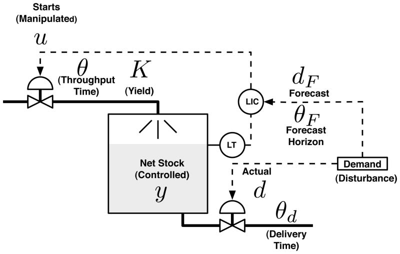
The production-inventory system is a classical problem in enterprise systems that has application in many problem arenas. Figure 1 shows a diagram of a production-inventory system under combined feedback-feedforward control action. The production node is represented by a pipe, while the inventory component consists of fluid in a tank. The goal is to manipulate the inflow to the production node (i.e., starts) in order to replenish an inventory that satisfies exogeneous demand. The demand signal is broken down into forecasted and unforecasted components. A substantial literature exists that examines production-inventory systems from a control engineering standpoint [11], [12], [13], [14]; recently, [15] examined both internal model control (IMC) and model predictive control (MPC) for a linear production-inventory system with continuous inputs. The hybrid production-inventory system, in which production occurs at discrete levels (or is decided by discrete-event decisions) is an important yet less examined problem; we consider it the focus of this paper.

Fig. 1.

Diagrammatical representation for a classical production-inventory system under combined feedback-feedforward control.

This paper highlights two distinct application areas that can be described as hybrid production-inventory systems. The first is adaptive interventions in behavioral health, which is a topic receiving increasing attention as a means to address the prevention and treatment of chronic, relapsing disorders, such as drug abuse [16]. In an adaptive intervention, dosages of intervention components (such as frequency of counseling visits or medication) are assigned to participants based on the values of tailoring variables that reflect some measure of outcome or adherence. Recent work has shown the relationship between forms of adaptive interventions and dynamical modeling and control of production-inventory systems [17], [18], [19]; [20] presents a risk-based model predictive control approach to the problem. In practice, these problems are hybrid in nature because dosages of intervention components correspond to discrete values. These interventions have to be implemented on a participant population that may display significant levels of interindividual variability. Hence a robust problem formulation is necessary that insures that the decision policy makes appropriate decisions for all members of a population, without demanding excessive modeling effort for each individual participant.

Inventory management in supply chains also represents a fertile application area for hybrid production-inventory systems. Prior work has established the benefits of a control engineering approach over classical Economic Order Quantity (EOQ) inventory management policies [15], [21], [22], [23], [24]; [15] in particular applies Monte Carlo simulation to demonstrate the improved performance and robustness of MPC over a smoothing replenishment rule representing an advanced “order-up-to” strategy [25]. The scenario considered in this paper is that of an enterprise that must make decisions on the startup and shutdown of an auxiliary manufacturing facility in order to accomplish operational goals under changing market demand. The problem is hybrid in nature, and the dynamics of this system can be highly uncertain [26]. Its solution calls for a novel problem formulation to insure efficient use of resources and an optimal operating policy for the inventory management problem, while accounting for changing market demand.

This paper presents an improved formulation of model predictive control (MPC) for linear hybrid systems that is amenable to achieving robust performance. The proposed scheme extends the use of mixed logical and dynamical (MLD) framework [1] for the control of hybrid systems subjected to measured and unmeasured disturbances and plant-model mismatch. The formulation offers a three-degree-of-freedom tuning for linear hybrid systems that addresses the requirements of setpoint tracking, measured (anticipated) disturbance rejection, and unmeasured disturbance rejection in the closed-loop system. This multi-degree-of-freedom formulation is patterned after the work of Wang and Rivera [26], which relies on the filter parametrization developed by Lee, Morari and García [27] and Lee and Yu [28] for unmeasured disturbance rejection in non-hybrid discrete-time systems. Tuning parameters are used in lieu of weights for independently adjusting the speeds of setpoint tracking and disturbance rejection (both measured and unmeasured) for each output of the closed-loop system. Systems with and without integrating dynamics are considered to accommodate a broad base of application settings and practical performance requirements. The paper extends the presentation in [29] with additional details, as well as describes a supply chain application, thus expanding the relevance of the approach to a broader class of problems.

The paper is organized as follows: Section 2 develops the MPC formulation with the multi-degree-of-freedom tuning for MLD systems. An example relying on the classical production-inventory system from Figure 1 but with discrete production levels is used to exemplify the algorithm and the three-degree-of-freedom tuning philosophy. Two case studies, namely a hypothetical adaptive intervention based on Fast Track program, and the supply chain management problem described previously are discussed in Section 3. Summary, conclusions, and directions for future research are presented in Section 4.

II. Model Predictive Control for Hybrid Systems

Model predictive control (MPC) is a form of closed-loop control where the current value of the manipulated variables is determined online as the solution of an optimal control problem over a horizon of given length [30]. The behavior of the system over the horizon is predicted with a model and the current plant state estimate assumed as the initial state for this prediction. When information about the plant state is available at the next sampling instant, the model is updated and optimization repeated over a shifted horizon. The ability to systematically include constraints and plants with multiple inputs and outputs, the flexibility given to the user to define a cost function, and the disturbance rejection properties of MPC have made it an attractive technique in the process industries, and beyond [31].

This section describes the model form and algorithm which incorporates the three degree-of-freedom formulation; it applies to any MLD model. The section concludes with an illustrative example from a standard production-inventory system with discrete-level production starts.

A. Process Model

The MPC controller presented in this paper uses a MLD-based model framework [1] represented as follows,

$$x(k)=Ax(k-1)+B_{1}u(k-1)+B_2\delta (k-1)+B_{3}z(k-1)+B_{d}d(k-1)$$ (1)

$$y(k)=Cx(k)+d^{\prime }(k)+\nu (k)$$ (2)

$$E_5\ge E_2\delta (k-1)+E_{3}z(k-1)-E_{4}y(k-1)-E_{1}u(k-1)+E_{d}d(k-1)$$ (3)

where $x={[\begin{array}{cc}{x}_c^T& x_d^T\end{array}]}^T,x_c\in {ℝ}^{n_x^c},x_d\in {\{0,1\}}^{n_x^d}$ and $u={[\begin{array}{cc}{u}_c^T& u_d^T\end{array}]}^T,u_c\in {ℝ}^{n_u^c},u_d\in {\{0,1\}}^{n_u^d},n_u\triangleq n_u^c+n_u^d$ represent states (both discrete and continuous) and inputs (both discrete and continuous) of the system. y ∈ ℝ^n_y is a vector of outputs, and d, d′ and ν represent measured disturbances, unmeasured disturbances and measurement noise signals, respectively. δ ∈ {0, 1}^n_d and z ∈ ℝ^n_z are discrete and continuous auxiliary variables that are necessary in order to incorporate logical/discrete decisions via linear inequality constraints; these are represented by Equation (3). The dimension of these auxiliary variables and the number of linear constraints in (3) depends on the specific character of the discrete logical/discrete decisions that have to be enforced in the particular hybrid system. The conversion of logical/discrete decisions into (3) using auxiliary variables is given by Bemporad and Morari [1] in detail. In particular, Bemporad and Morari [1] rely on propositional calculus and Big-M constraints [32] to express discrete actions in terms of (3). The framework permits the user to include and prioritize constraints as well as incorporate heuristic rules in the description of the model. Because disturbances are an inherent part of any system, it is necessary to incorporate these in the controller model. Equations (1)–(3) extend the MLD framework shown in [1] through the inclusion of measured and unmeasured disturbances. Furthermore, the model lumps the effect of all unmeasured disturbances on the outputs only, which is a common practice in the process control literature [26], [28]. We consider d′, the unmeasured disturbance, as a stochastic signal described by the model,

$$x_w(k)=A_w{x}_w(k-1)+B_{w}w(k-1)$$ (4)

$$d^{\prime }(k)=C_w{x}_w(k)$$ (5)

A_w has all eigenvalues inside the unit circle while w(k) is a vector of integrated white noise. Here it is assumed that the disturbance vector d′ consists of uncorrelated components. Consequently, B_w = C_w = I and A_w = diag{α₁, α₂, ···, α_ny} where α_i = 1, i = 1, 2, ···, n_y for doubly-integrated (i.e., Type II, per [33]) disturbances, while α_i = 0, i = 1, 2, ···, n_y for single-integrating (i.e., Type I) disturbances. n_y corresponds to the total number of outputs. In order to take advantage of the well understood properties of white noise signals, we consider differenced forms of the disturbance and system models and augment them as follows,

$$X(k)=\mathcal{A}X(k-1)+{\mathcal{B}}_1\mathrm{\Delta }u(k-1)+{\mathcal{B}}_2\mathrm{\Delta }\delta (k-1)+{\mathcal{B}}_3\mathrm{\Delta }z(k-1)+{\mathcal{B}}_d\mathrm{\Delta }d(k-1)+{\mathcal{B}}_w\mathrm{\Delta }w(k-1)$$ (6)

$$y(k)=\mathcal{C}X(k)+\nu (k)$$ (7)

where,

$$\begin{array}{l}X(k)={[\begin{array}{ccc}\mathrm{\Delta }{x}^T(k)& \mathrm{\Delta }{x}_w^T(k)& y^T(k)\end{array}]}^T\\ \mathcal{A}=\left[\begin{array}{ccc}A& 0& 0\\ 0& A_w& 0\\ CA& A_w& I\end{array}\right];{\mathcal{B}}_i=\left[\begin{array}{c}{B}_i\\ 0\\ {CB}_i\end{array}\right],i=1,2,3,d;{\mathcal{B}}_w=\left[\begin{array}{c}0\\ I\\ I\end{array}\right];\mathcal{C}=[\begin{array}{ccc}0& 0& I\end{array}]\end{array}$$

Here Δ * (k) = *(k) − *(k − 1) and Δw(k) is a white noise sequence.

B. MPC Problem

In this work, we rely on a quadratic cost function of the form,

$$\begin{array}{l}J\triangleq \sum _{i=1}^p{\Vert (y(k+i)-y_r)\Vert }_{Q_y}^2+\sum _{i=0}^{m-1}{\Vert (\mathrm{\Delta }u(k+i))\Vert }_{Q_{\mathrm{\Delta }u}}^2\\ +\sum _{i=0}^{m-1}{\Vert (u(k+i)-u_r)\Vert }_{Q_u}^2+\sum _{i=0}^{p-1}{\Vert (\delta (k+i)-{\delta }_r)\Vert }_{Q_d}^2+\sum _{i=0}^{p-1}{\Vert (z(k+i)-z_r)\Vert }_{Q_z}^2\end{array}$$ (8)

The optimization problem consists of finding the sequence of control actions u(k), …, u(k+m−1), d(k), …, d(k+ p − 1), and z(k), …, z(k + p − 1) that minimize J

$$\underset{\{{[u(k+i)]}_{i=0}^{m-1},{[\delta (k+i)]}_{i=0}^{p-1},{[z(k+i)]}_{i=0}^{p-1}\}}{min}J$$ (9)

subject to mixed integer constraints according to (3) and various process constraints,

$$y_{min}\le y(k+i)\le y_{max},1\le i\le p$$ (10)

$$u_{min}\le u(k+i)\le u_{max},0\le i\le m-1$$ (11)

$$\mathrm{\Delta }{u}_{min}\le \mathrm{\Delta }u(k+i)\le \mathrm{\Delta }{u}_{max},0\le i\le m-1$$ (12)

p is the prediction horizon and m is the control horizon. u_min, u_max, and y_min, y_max are lower and upper bound on inputs and outputs, respectively. (·)_r stands for reference, ${\Vert (·)\Vert }_{Q_{\ast }}\triangleq \sqrt{{(·)}^T{Q}_{\ast }(·)}$ is the vector 2-norm weighted by matrix Q_* and Q_y, Q_Δu, Q_u, Q_d, and Q_z are penalty weights on the control error, move size, control signal, auxiliary binary variables and auxiliary continuous variables, respectively. The objective function in (8) corresponds to that used by Bemporad and Morari [1] with the additional term of move suppression (the penalty term on Δu). In most practical problems, only the first three terms of the objective function (control error, move size, control signal) are considered; however, in keeping with [1] and to maintain generality of the MPC formulation, we include the last two terms that minimize the error of the auxiliary variables δ and z from user-specified reference values. Moreover, the objective function (8) and the linear hybrid system described by the MLD model (1)–(3) are governed by both binary and continuous variables. Consequently, (8) along with the linear hybrid system dynamics (1)–(3) and linear inequality constraints described in (10)–(12), the solution to (9) forms a mixed integer quadratic program (miqp).

The MPC problem described by (8)–(12) requires future predictions of the outputs and the mixed integer constraints in (3). The future predictions can be obtained by propagating (6), (7) and (3) for p steps in future, resulting in the following prediction equations,

$$\begin{array}{c}\mathcal{Y}(k+1)=\mathrm{\Phi }X(k)+{\mathcal{H}}_1\mathcal{U}(k)+{\mathcal{H}}_2\overline{\delta }(k)+{\mathcal{H}}_3\mathcal{Z}(k)+{\mathcal{H}}_d\mathcal{D}(k)-H_{11}u(k-1)\\ -H_{21}\delta (k-1)-H_{31}z(k-1)-H_{d1}{d}_{\mathit{flt}}(k-1)\end{array}$$ (13)

$${\overline{E}}_5\ge {\overline{E}}_2\overline{\delta }(k)+{\overline{E}}_3\mathcal{Z}(k)+{\overline{E}}_1\mathcal{U}(k)+{\overline{E}}_4\mathcal{Y}(k)+{\overline{E}}_d\mathcal{D}(k)$$ (14)

Equation (14) can be further simplified by substituting (k) and rewriting as,

$$\begin{array}{c}{\mathcal{E}}_5\ge {\mathcal{E}}_2\overline{\delta }(k)+{\mathcal{E}}_3\mathcal{Z}(k)+{\mathcal{E}}_1\mathcal{U}(k)+{\mathcal{E}}_{4}X(k)+{\mathcal{E}}_d\mathcal{D}(k)-{\mathcal{E}}_{41}u(k-1)\\ -{\mathcal{E}}_{42}\delta (k-1)-{\mathcal{E}}_{43}z(k-1)-{\mathcal{E}}_{4d}{d}_{\mathit{flt}}(k-1)\end{array}$$ (15)

where d_flt represents the filtered value of the measured disturbance obtained using a discrete time filter; this is discussed in more detail in the next section. (k + 1), (k),δ̄(k), (k) and (k) are future values of outputs, inputs, auxiliary binary variables, auxiliary continuous variables and filtered measured disturbances as given below:

$$\mathcal{Y}(k+1)={[y^T(k+1)y^T(k+2)\cdots y^T(k+p)]}^T$$ (16)

$$\mathcal{U}(k)={[u^T(k)\cdots u^T(k+m-1)]}^T$$ (17)

$$\overline{\delta }(k)={[{\delta }^T(k)\cdots {\delta }^T(k+p-1)]}^T$$ (18)

$$\mathcal{Z}(k)={[z^T(k)\cdots z^T(k+p-1)]}^T$$ (19)

$$\mathcal{D}(k)={[{d_{\mathit{flt}}}^T(k)\cdots {d_{\mathit{flt}}}^T(k+p-1)]}^T$$ (20)

Φ, , H_*, and Ē_* are the appropriate coefficients matrices that can be generated using (3), (6) and (7); these are given in Appendix-A. , δ̄ and are the decision variables of the MPC problem described in (8)–(12) and can be found by an miqp optimizer. is an externally generated forecast of the measured disturbances values that is provided externally to the algorithm. Using (13)–(20), the MPC problem in (8)–(12) can be rewritten in vector form as

$$\underset{\{\mathcal{U}(k),\overline{\delta }(k),\mathcal{Z}(k)\}}{min}J\triangleq {\Vert (\mathcal{Y}(k+1)-{\mathcal{Y}}_r)\Vert }_{{\widehat{Q}}_y}^2+{\Vert (R_u\mathcal{U}(k)-R_{u0}u(k-1))\Vert }_{{\widehat{Q}}_{\mathrm{\Delta }u}}^2+{\Vert (\mathcal{U}(k)-{\mathcal{U}}_r)\Vert }_{{\widehat{Q}}_u}^2+{\Vert (\overline{\delta }(k)-{\overline{\delta }}_r)\Vert }_{{\widehat{Q}}_d}^2+{\Vert (\mathcal{Z}(k)-{\mathcal{Z}}_r)\Vert }_{{\widehat{Q}}_z}^2$$ (21)

subject to mixed integer constraints according to (15) and various process constraints,

$${\mathcal{Y}}_{min}\le \mathcal{Y}(k+1)\le {\mathcal{Y}}_{max}$$ (22)

$${\mathcal{U}}_{min}\le \mathcal{U}(k)\le {\mathcal{U}}_{max}$$ (23)

$$\mathrm{\Delta }{\mathcal{U}}_{min}\le \mathrm{\Delta }\mathcal{U}(k)\le \mathrm{\Delta }{\mathcal{U}}_{max}$$ (24)

where,

$${\widehat{Q}}_{\ast }=\left[\begin{array}{cccc}{Q}_{\ast }& 0& ·& 0\\ ⋮& \ddots & ·& ⋮\\ 0& \cdots & ·& Q_{\ast }\end{array}\right];R_u=\left[\begin{array}{ccccc}I& 0& \cdots & 0& 0\\ -I& I& \cdots & 0& 0\\ 0& -I& \ddots & ⋮& ⋮\\ ⋮& ⋮& \ddots & \ddots & ⋮\\ 0& 0& \cdots & -I& I\end{array}\right];R_{u0}=\left[\begin{array}{c}I\\ 0\\ ⋮\\ 0\end{array}\right]$$

, , δ̄_r and are the reference vectors for the outputs, inputs, auxiliary binary variables and auxiliary continuous variables as given below:

$${\mathcal{Y}}_r={[y_r^T(k+1)y_r^T(k+2)\cdots y_r^T(k+p)]}^T$$ (25)

$${\mathcal{U}}_r={[u_r^T(k)u_r^T(k+1)\cdots u_r^T(k+m-1)]}^T$$ (26)

$${\overline{\delta }}_r={[{\delta }_r^T(k){\delta }_r^T(k+1)\cdots {\delta }_r^T(k+p-1)]}^T$$ (27)

$${\mathcal{Z}}_r={[z_r^T(k)z_r^T(k+1)\cdots z_r^T(k+p-1)]}^T$$ (28)

Substituting (13) for (k + 1) into (21) and rearranging the objective function in (21) (such that one group consist of all the quadratic terms of the decision variables, while the other group consists of all the linear terms) with constraints described in (15) and (22)–(24) leads to defining the MPC problem into a standard mixed integer quadratic program (miqp) as follows:

$$\underset{\xi }{min}J\triangleq \frac{1}{2}{\xi }^T\mathcal{H}\xi +{\mathcal{G}}^T\xi$$ (29)

$$\mathcal{S}\xi \le b$$ (30)

where ξ = [ (k)^T δ̄(k)^T (k)^T]^T is the vector of the decision variables, and are coefficient matrices for the quadratic and linear terms of the objective function, respectively, and and b represent the coefficient matrices for the linear constraints. The coefficient matrices , , and b are defined using Φ, , H_*, and Ē_* and are given in Appendix-B. Thus (29)–(30) represent the MPC control law for linear hybrid systems with measured and unmeasured disturbances, which consists of a standard miqp problem. The size of this problem will vary with the number of inputs (u), auxiliary variables (δ and z), and mixed integer constraints in (3), as well as the length of the prediction (p) and control (m) horizons. For a particular linear hybrid system the size of the miqp problem considered here will be similar to that obtained from [1]. The tremendous advances in miqp solution techniques and commercialized solvers make it possible to solve moderate to large size miqp problems in real-time. While any miqp solver available in the market should be suitable, in this work, we have relied on the TOMLAB-CPLEX solver. Alternatively, one can also opt for a multiparametric approach ([34]) that gives an explicit solution for the constrained miqp and thus reduces the computational time.

The nominal stability and convergence properties of MPC using MLD models are discussed extensively in [1]; Theorem 1 in [1] indicates that the choice of objective function weights will guarantee stability and convergence. Because the proposed MPC algorithm is based on a MLD model description with a similar objective function to [1], these properties apply as well to the problem formulation presented in this paper. It should be noted that our algorithm relies on externally generated reference trajectories, forecasts of the measured disturbances, and estimates of (disturbance-free) initial states X(k) to achieve nominal and robust performance; these considerations are discussed in the ensuing section.

C. Three-Degree-of-Freedom Tuning Parameters

The MPC formulation considered in this work features three-degree-of-freedom tuning where the performance requirements associated with setpoint tracking, unmeasured disturbance rejection, and anticipated measured disturbance rejection can be adjusted independently. This multiple-degree-of-freedom functionality influences the controller response more intuitively and conveniently than the traditional approach of adjusting penalty weights in the objective function; this is developed as follows:

1. Reference Trajectory and Setpoint Tracking: The output reference trajectory is generated using the filter

   $$\frac{y_r(k+i)}{y_{\mathit{target}}}=f(q,{\alpha }_r^j),1\le j\le n_y,1\le i\le p$$ (31)
   where $f(q,{\alpha }_r^j)$ is a Type-I discrete-time filter for the j-th reference as given in [33]

   $$f(q,{\alpha }_r^j)=\frac{(1-{\alpha }_r^j)q}{q-{\alpha }_r^j},1\le j\le n_y$$ (32)

   and q is the forward shift operator. The speed of setpoint tracking can be adjusted by choosing ${\alpha }_r^j$ between [0,1) for each individual output j. The smaller the value for ${\alpha }_r^j$, the faster the output response for setpoint tracking. This adjustment is more intuitive than adjusting move suppression weights (Q_Δu) that directly affect the manipulated variables and consequently, the effect on a specific controlled variable response is more difficult to predict. We note that the reference trajectories for the inputs and auxiliary binary and continuous variables ( , δ̄_r and ) are considered constant over the prediction horizon at their respective predefined target values.

2. Measured Disturbance Rejection: The proposed formulation relies on an externally generated forecast of the measured disturbance as in (20); this forecast is filtered and provided as an anticipated signal to the control algorithm. The speed desired to reject measured disturbances can be adjusted independently by using a filter $f(q,{\alpha }_d^j)$, 1 ≤ j ≤ n_dist for each measured disturbance signal. Here n_dist is the number of measured disturbances and ${\alpha }_d^j$ is a tuning parameter whose value lies between [0,1), for each j-th measured disturbance. The lower the value for ${\alpha }_d^j$, the faster the speed of disturbance rejection. The form of the transfer function $f(q,{\alpha }_d^j)$ required depends on whether the disturbance is an asymptotically step or ramp (i.e., Type-I or Type-II signal, as defined in [33]). A Type-II filter structure should be used when integrating system dynamics are present [26]. The Type-I filter structure is given in (32) and the Type-II filter structure is given as follows [33]:

   $$f(q,{\alpha }_d^j)=({\beta }_0+{\beta }_1{q}^{-1}+\cdots +{\beta }_{\omega }{q}^{-\omega })\times \frac{(1-{\alpha }_d^j)q}{q-{\alpha }_d^j}$$ (33)

   $${\beta }_k=\frac{-6k{\alpha }_d^j}{(1-{\alpha }_d^j)\omega (\omega +1)(2\omega +1)},1\le k\le \omega$$ (34)

   $${\beta }_0=1-({\beta }_1+\cdots +{\beta }_{\omega })$$ (35)
3. Unmeasured Disturbance Rejection: The proposed MPC problem (29)–(30) requires calculating the coefficient matrix for the linear term of the objective function (29) and the right-hand side of constraint equation (30) (b) at each time step. This requires initial states X(k) of the augmented system at each time instance. The augmented states X(k) can be estimated from the current measurements y(k) with unmeasured disturbance rejection achieved by a suitably designed state observer/filter. In order to decouple the effects of measured and unmeasured disturbance rejection and true multiple degree-of-freedom tuning for these controller modes, we propose a two-step procedure for estimating the augmented states X(k). In the first step, state estimation is accomplished utilizing the model, the actual (unfiltered) measured disturbance signal d, and a filter K_f as follows,

   $$X(k\mid k-1)=\mathcal{A}X(k-1\mid k-1)+{\mathcal{B}}_1\mathrm{\Delta }u(k-1)+{\mathcal{B}}_2\mathrm{\Delta }\delta (k-1)+{\mathcal{B}}_3\mathrm{\Delta }z(k-1)+{\mathcal{B}}_d\mathrm{\Delta }d(k-1)$$ (36)

   $$X(k\mid k)=X(k\mid k-1)+K_f(y(k)-\mathcal{C}X(k\mid k-1))$$ (37)
   Since we rely on the unfiltered measured disturbance d in (36), the second term in (37) represents the effect of unmeasured disturbances only; the choice for K_f will define the speed and character of unmeasured disturbance rejection. Next, we estimate an augmented state of the system by considering the filtered measured disturbance signal d_flt and the contribution of the unmeasured disturbance (i.e., the prediction error) from (37) as follows,

   $$X_{\mathit{flt}}(k\mid k-1)=\mathcal{A}{X}_{\mathit{flt}}(k-1\mid k-1)+{\mathcal{B}}_1\mathrm{\Delta }u(k-1)+{\mathcal{B}}_2\mathrm{\Delta }\delta (k-1)+{\mathcal{B}}_3\mathrm{\Delta }z(k-1)+{\mathcal{B}}_d\mathrm{\Delta }{d}_{\mathit{flt}}(k-1)$$ (38)

   $$X_{\mathit{flt}}(k\mid k)=X_{\mathit{flt}}(k\mid k-1)+K_f(y(k)-\mathcal{C}X(k\mid k-1))$$ (39)
   The first term of (39) captures the effect of the filtered measured disturbances, while the second term (which is same as in (37)) captures the effect of the unmeasured disturbances. Thus, X_flt(k|k) accounts for the both filtered measured and unmeasured disturbances such that the measured disturbance tuning specified through ${\alpha }_d^j$ does not influence unmeasured disturbance rejection, while the unmeasured disturbance filter matrix K_f does not affect measured disturbance rejection. Finally, X_flt(k|k) is used in (B.2) and (B.4) to calculate the coefficient matrices and b that appear in the MPC problem (29)–(30). The optimal value of the filter gain K_f could be found by solving an algebraic Riccati equation; however, this will require estimating covariance matrices for the unmeasured disturbance and measurement noise, which may not be known accurately. Instead, we rely on the parametrization shown in Lee, Morari, and García [27] and Lee and Yu [28], which, in keeping with the setpoint tracking and measured disturbance modes, enables specifying the speed of unmeasured disturbance rejection for each output channel independently by the user. For the case of A_w = diag{α₁, α₂, ···, α_ny}, we apply the following parametrization of the filter gain:

   $$K_f=\left[\begin{array}{c}0\\ F_b\\ F_a\end{array}\right]$$ (40)
   where

   $$F_a=\text{diag}\{{(f_a)}_1,\cdots ,{(f_a)}_{n_y}\}$$ (41)

   $$F_b=\text{diag}\{{(f_b)}_1,\cdots ,{(f_b)}_{n_y}\}$$ (42)

   $${(f_b)}_j=\frac{{{(f_a)}_j}^2}{1+{\alpha }_j-{\alpha }_j{(f_a)}_j},1\le j\le n_y$$ (43)

   (f_a)_j is a tuning parameter that lies between 0 and 1; the speed of unmeasured disturbance rejection is proportional to the tuning parameter (f_a)_j. As (f_a)_j approaches zero, the state estimator increasingly ignores the prediction error correction, and the control solution is mainly determined by the deterministic model (36) and the the feedforward anticipation signal. On the other hand, the state estimator tries to compensate for all prediction error as (f_a)_j approaches 1, and consequently the controller becomes extremely aggressive. Thus, by adjusting (f_a)_j, the user can directly influence unmeasured disturbance rejection for each output response individually, which is more intuitive than tuning with move suppression in the traditional MPC formulation.

   It should be noted that the MLD model presented in (1)–(3) can also accommodate discrete outputs. However, in this work we assume that all output signals are continuous. The filter gain matrix K_f is parameterized such that the elements corresponding to Δx(k) (which can consist of continuous as well discrete states of the system) is always 0; this is observed from (40). Hence, the original system states x(k) are never corrected for unmeasured disturbances; only the outputs y(k) are corrected for the cumulative effect of all the disturbances in the process. Thus, the proposed MPC formulation yields offset-free responses in the presence of the asymptotically ramp disturbances or asymptotically step disturbances on the outputs by choosing A_w = I or A_w = 0, respectively. This requires measurements of all the controlled outputs. Furthermore, the controller is able to reject asymptotically ramp disturbances because of the integral action resulting from the use of the augmented model in the difference form with A_w = I.

4. Robustness considerations: Addressing performance-robustness tradeoffs is a fundamental consideration in tuning MPC controllers [35]. In the three degree-of-freedom formulation, plant-model mismatch is experienced by the control system as an unmeasured disturbance, and consequently the tuning of the unmeasured disturbance mode through (f_a)_j will dictate the controller response to model uncertainty [15], [36]. The robustness of the filter according to (36)–(43) under unconstrained conditions for linear continuous (non-hybrid) systems is examined in detail by Lee and Yu [28]. Lee and Yu [28] show the direct relationship between the shape and bandwidth of the sensitivity and complementary sensitivity functions for various settings of (f_a)_j and α_i, and how formal robustness guarantees for this controller can be determined using the concept of the Structured Singular Value [37]. For the constrained case with discrete decision variables, formally assessing the robustness of MPC represents a much greater challenge, although some intutive approaches can be taken [38]. A formal proof of the effect of these tuning and disturbance parameters on robustness for a hybrid, constrained system lies beyond the scope of this paper; however, because of the direct connection between the value of (f_a)_j and closed-loop bandwidth, it is expected that robustness at the expense of performance will be obtained as (f_a)_j approaches 0. Both a simulation example (presented in the next subsection) as well as Case Study I in Section III.A are provided in support of this claim.

D. Example: Production-Inventory System

As an illustration of the algorithm we consider a classical production-inventory system (Fig. 1), the basic node of a supply chain [15]. This system can be modeled using a fluid analogy where the inventory is represented as a tank containing fluid, while the production node is represented as a pipe with throughput time θ = θ′ + 1 sampling instants and yield K. The net stock y(k) representing fluid level and the inlet pipe flow u(k) representing factory starts are the controlled and manipulated variables, respectively. The outlet flow represents the demand d(k) that is composed of an unforecasted component d_u(k) and a forecasted component d_f (k − θ_f), with θ_f representing the forecast time. The dynamics of this system are given by an overall mass balance as follows,

$$y(k+1)=y(k)+Ku(k-{\theta }^{\prime })-d(k)$$ (44)

where d(k) = d_f (k − θ_f) + d_u(k) is the total customer demand. The operational goal of this system is to meet the customer demand d(k) while maintaining the net stock inventory level at a predefined target. This can be accomplished by manipulating factory starts u(k) and feedforward compensation of forecasted demand d_f (k). In this example, the manipulated input u(k) is restricted to assume only four values: 0, 33.33, 66.66 and 100. Thus, the plant according to (44) is a class of hybrid system with discrete inputs and continuous output y(k) which can be modeled using the MLD representation described by (1)–(3). In order to capture discreteness in the input, four binary auxiliary variables (δ₁, δ₂, δ₃, δ₄) and three continuous auxiliary variables (z₁, z₂, z₃) are introduced with the following relationships:

$${\delta }_1(k)=1\iff z_1(k)=100$$ (45)

$${\delta }_2(k)=1\iff z_2(k)=66.66$$ (46)

$${\delta }_3(k)=1\iff z_3(k)=33.33$$ (47)

$$\sum _{i=1}^4{\delta }_i(k)=1$$ (48)

$$u(k)=\sum _{i=1}^3{z}_i(k)$$ (49)

The symbol “⇔” should be read as if and only if (e.g. δ₁ = 1 if and only if z₁ = 100 else 0 or viceversa). The conditions in (45)–(49) insure that the input u(k) takes only one of four possible values at a particular time instant. The implication (⇔) in (45)–(47) can be converted into linear inequality constraints using equivalence with propositional logic [32] followed by matrix representation as in (3). This yields a mixed logical dynamical (MLD) model for the production-inventory problem discussed above. The MLD model can then be used to formulate an MPC problem of the form (29)–(30). In this case we consider a sampling interval of T = 1 day, θ_f = p = 30 days, system gain K = 0.9 and throughput time of four (θ′ = 3) days.

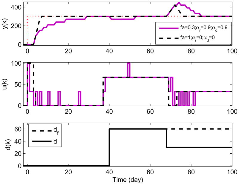
Figure 2 shows how the parameters α_r, α_d and f_a can be manipulated to affect the nominal speed of response and hence the robustness of the algorithm. As noted previously, the speeds of setpoint tracking and measured disturbance rejection are inversely proportional to the values of α_r and α_d, respectively, while the speed of unmeasured disturbance rejection is proportional to the value of f_a. Initially, a step setpoint change of magnitude 300 is introduced. The solid line represent the controller performance for the three-degree-of-tuning parameters α_r = 0.9, α_d = 0.9 and f_a = 0.3, while the dashed lines represent the controller performance for the parameters α_r = 0, α_d = 0 and f_a = 1. It can be seen that the system achieves faster setpoint tracking for α_r = 0 as compared to α_r = 0.9. At day 40, a step change of magnitude 60 occurs in the customer demand d(k), which is forecasted without error (i.e., d(k) = d_f (k) = 60) until day 67. For α_d = 0, the controller is able to quickly notice a change in the demand and takes an early feedforward action in order to maintain the inventory at the setpoint without any deviation (dashed line). On the other hand, for α_d = 0.9, the rate of production slows down, resulting in a dip in inventory (solid line). At day 68, demand suddenly decreases to 30 from 60. This change in the demand yields a negative bias of 30 units in the forecast that can be considered as an unmeasured disturbance (i.e., d_u(k) = d(k)−d_f (k) = −30). In this case, feedback action is taken by the controller and by the time the controller realizes the decrease in demand, inventory has exceeded the setpoint. As a consequence of continued control action, the system response eventually settles at the setpoint. Faster unmeasured disturbance rejection is accomplished for f_a = 1 than for f_a = 0.3. The simulation results show how the adjustable parameters α_r, α_d and f_a have an intuitive effect on the closed-loop response of the production-inventory system, and can be selected by the user to achieve desired levels of performance and robustness.

Fig. 2.

Evaluation of tuning parameters, classical production-inventory example: (i) dashed line: α_r = 0, α_d = 0., f_a = 1 (ii) solid line: α_r = 0.9, α_d = 0.9, f_a = 0.3. The bottom panel shows a measured disturbance d_f (k) and an unmeasured disturbance d_u(k) that enter at days 40 and 53, respectively. The solid black line represents the total disturbance d(k), while the dashed line represents the disturbance forecast.

III. Case Studies

In this section, we examine the efficacy of the proposed algorithm on case studies taken from two non-traditional applications for control systems engineering: adaptive behavioral interventions and inventory management in supply chains. While appearing on the surface as distinct (and unrelated) application areas, both of these problems can be abstracted as hybrid production-inventory control systems, and consequently stand to benefit from the general hybrid MPC problem formulation developed in this paper. The case study on adaptive interventions (Section III.A) illustrates for the case of a discrete input the benefits of the multiple degree-of-freedom formulation on a problem involving significant uncertainty. Meanwhile, the supply chain case study (Section III.B) illustrates the benefits of the algorithm for problems involving a discrete decision based on the value of the outputs, and under circumstances when both measured and unmeasured disturbances (requiring combined feedback and feedforward control action) are present. In both case studies a comparison is made to hybrid MPC tuning using only objective function weights, without independent degrees-of-freedom.

A. Adaptive Behavioral Interventions

As a representative case study of a time-varying adaptive behavioral intervention we examine a hypothetical intervention based on the Fast Track program [39]. Fast Track was a multi-year, multi-component program designed to prevent conduct disorder in at-risk children. Youth showing conduct disorder are at increased risk for incarceration, injury, depression, substance abuse, and death by homicide or suicide. In Fast Track, some intervention components were delivered universally to all participants, while other specialized components were delivered adaptively. In this paper we focus on the adaptive intervention scenario described in [16] for assigning family counseling, which was provided to families on the basis of parental functioning. There are several possible levels of intensity, or doses, of family counseling. The idea is to vary the dose of family counseling depending on the needs of the family, in order to avoid providing an insufficient amount of counseling for very troubled families, or wasting counseling resources on families that may not need them or be stigmatized by excessive counseling. The decision about which dose of counseling to offer each family is based primarily on the family’s level of functioning, assessed by a questionnaire completed by the parents. As described in [16], based on the questionnaire and the clinician’s assessment, parental function is determined to fall in one of the following categories: very poor, poor, near threshold, or at/above threshold. A traditional approach in behavioral health is to adapt the intervention through a set of simple “IF-THEN” decision rules that are applied as follows: families with very poor functioning are given weekly counseling; families with poor functioning are given biweekly counseling; families with near threshold functioning are given monthly counseling; and families at or above threshold are given no counseling. Family functioning is reassessed at a review interval of three months, at which time the intervention dosage may change. This process goes on for three years, with twelve opportunities for a dose of family counseling to be assigned.

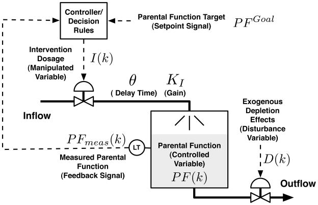
Rivera et al. [17] examine the links between adaptive behavioral interventions and feedback control systems, proposing means by which a control system engineering approach can optimize the delivery of these interventions. The approach followed in [17] models the intervention using a fluid analogy, represented in Figure 3. Parental function PF(k), the controlled variable, is treated as liquid in a tank, which is depleted by exogenous disturbances D(k). The tank is replenished by the intervention I(k), which is the manipulated variable. The use of a fluid analogy enables developing a mathematical model of the open-loop dynamics of the intervention using the principle of conservation of mass. This model can be described by the following difference equations that relate parental function PF(k) with the intervention I(k):

$$PF(k+1)=PF(k)+K_{I}I(k-\theta )-D(k)$$ (50)

$$D(k)=\sum _{i=1}^{n_d}{D}_i(k)$$ (51)

$${PF}_{\mathit{meas}}(k)=PF(k)+N(k)$$ (52)

Fig. 3.

Fluid analogy corresponding to the hypothetical adaptive behavioral intervention. Parental function PF(k) is treated as material (inventory) in a tank, which is depleted by disturbances D(k) and replenished by intervention dosage I(k), which is the manipulated variable.

PF(k) is the parental function, I(k) refers to the intervention dosage (frequency of counselor home visits), K_I is the intervention gain, θ represent time delay between intervention and its effect on parental function, and PF_meas(k) is the parental function measurement. D(k) is the source of parental function depletion and N(k) represents the measurement noise. I(k), the frequency of counselor visits, has a restriction such that these can only be possible either weekly, biweekly, monthly, or none at all. This problem requires imposing a restriction on the intervention I(k) such that it takes only four values: 0, I^weekly, I^biweekly and I^monthly. Thus, the problem has inherent discreteness along with the continuous dynamics, which can be characterized by a hybrid dynamical system. The parental function system can be modeled using the MLD framework. In order to capture discreteness in the intervention, four binary auxiliary variables, δ₁, δ₂, δ₃, δ₄ and three continuous auxiliary variables, I₁, I₂, I₃ are introduced. The detailed description of the MLD model is not shown here but can be obtained by following a similar procedure as in the production-inventory example of Section II.D.

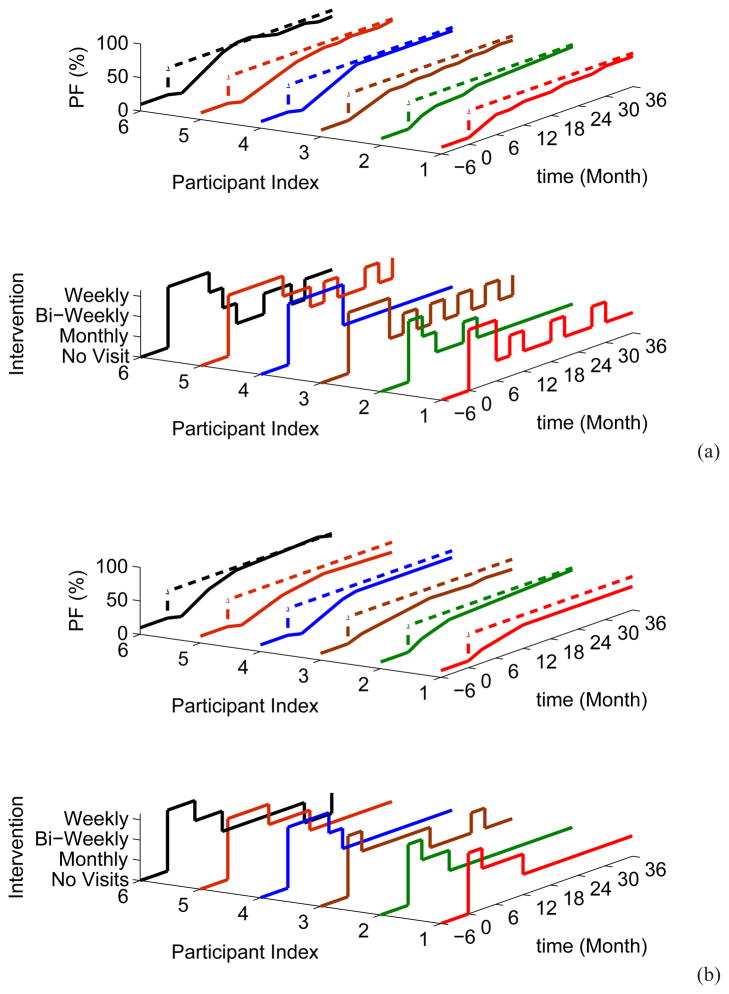
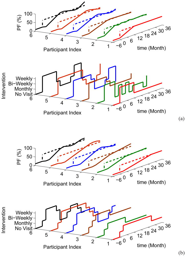
In the case study the controller is based on a nominal model with parameters K_I = 0.15 and θ = 0, prediction horizon p = 30 and control horizon m = 10. The TOMLAB-CPLEX solver is used to solve the resulting mixed integer quadratic program (miqp) optimization problem. Figure 4(a) documents the simulation results for various levels of gain and delay mismatch in the presence of a setpoint change in parental function to 50% and a simultaneous step unmeasured disturbance D(k) = 5 using the proposed MPC formulation. Tuning parameters Q_y = 1, Q_Δu = Q_u = Q_d = Q_z = 0, and (α_r, f_a) = (0, 0.3) are used for all the cases. α_d is not considered as this problem is feedback-only (i.e., no measured disturbance variables are considered). Six cases involving gain and delay mismatch (ΔK_I, Δθ) and representing intervention participant variability are evaluated, starting with case 1: (0, 0; nominal model, no mismatch), case 2: (21%, 0), case 3: (−15%, 0), case 4: (0%, 1), case 5: (−15%, 1), and case 6: (21%, 1). Various characteristics of the integrating system dynamics are reflected in these results. For example, a negative gain mismatch leads to sluggish response in parental function (case 3), while a positive gain mismatch yields faster response (case 2) than the nominal (case 1). On the other hand, mismatch in time delay is responsible for a slight overshoot in case 6. In spite of all these variations, the hybrid control system displays satisfactory performance in the face of significant plant-model mismatch, with stable and predominantly overdamped responses in the parental function response, displaying no offset for all the cases presented in this paper.

Fig. 4.

Evaluation of the hybrid MPC formulation with 3-DoF tuning parameters ((α_r, f_a) = (0, 0.3), Q_y = 1 and Q_Δu = 0, (a)) and the IF-THEN rule-based decision policy (b) for the counselor visits-parental function intervention under conditions of gain and delay mismatch. A setpoint change from 10% to 50% parental function with simultaneous step disturbance D(k) = 5 are evaluated under varying conditions of gain and delay mismatch (ΔK_I, Δθ): case 1 (nominal): (0, 0), case 2: (21%, 0), case 3: (−15%, 0), case 4: (0%, 1), case 5: (−15%, 1), case 6: (21%, 1).

In order to better appreciate the performance of the proposed three-degree-of freedom MPC formulation, we analyze the problem using the “IF-THEN “ rule-based decision policy [17] and an MPC formulation that relies on constant plant-model mismatch ((α_r, f_a) = (0, 1.0)), with and without move suppression Q_Δu. Fig. 4(b) displays the simulation results using the IF-THEN rule-based decision policy. These results show that the IF-THEN decision policy leads to significant offset for the first five cases, producing desirable performance only for case 6. This policy relies only on the current measurement of parental function and does not take into account the dynamic relationship between parental function and intervention dose, which accounts for the subpar performance. Figure 5(a) and Fig. 5(b) display the responses from an MPC formulation relying on constant plant-model mismatch over a prediction horizon for Q_Δu = 0 (no move suppression) and Q_Δu = 1, respectively. For the case of no move suppression (Q_Δu = 0, Fig. 5(a)), parental function achieves the desired goal without offset for all six cases. However, the controlled variable responses result in overshoot and oscillations for Cases 3 – 6, and the dosage assignments in general display wide variations that would not be well tolerated in a clinical setting. Applying Q_Δu = 1 attenuates the aggressive nature of the controller, but the last three cases still exhibit significant overshoot, and the controller settling times display the largest variation of all the control systems considered in the case study.

Fig. 5.

Evaluation of the hybrid MPC formulation relying on constant plant-model mismatch and move suppression for the counselor visits-parental function intervention under conditions of gain and delay mismatch. A setpoint change from 10% to 50% parental function with simultaneous step disturbance D(k) = 5 are evaluated under varying conditions of gain and delay mismatch (ΔK_I, Δθ): case 1 (nominal): (0, 0), case 2: (21%, 0), case 3: (−15%, 0), case 4: (0%, 1), case 5: (−15%, 1), case 6: (21%, 1). (a) Q_y = 1 and Q_Δu = 0 (b) Q_y = 1 and Q_Δu = 1.

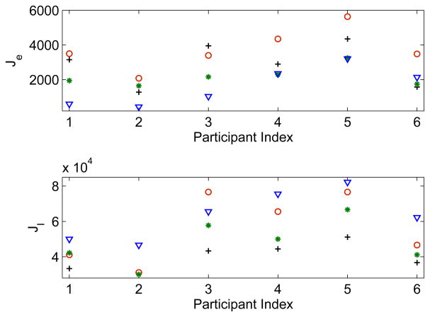
Figure 6 displays the values for the closed-loop performance metrics J_e and J_I that represent measures of cumulative deviation of parental function from the goal and cumulative intervention energy, respectively. J_e and J_I are defined as follows,

Fig. 6.

Comparison of the performance metrics J_e and J_I using the proposed MPC formulation (‘*’); MPC formulation assuming a constant plant-model mismatch over the prediction horizon (‘o’ for Q_Δu = 1 and ‘∇’ for Q_Δu = 0) and IF-THEN decision policy [17] (‘+’). Tuning parameters as in Figures 4 and 5.

$$J_e=\sum _{k=1}^{t/T_s}{(PF(k)-{PF}^{\mathit{goal}})}^T(PF(k)-{PF}^{\mathit{goal}})$$ (53)

$$J_I=\sum _{k=1}^{t/T_s}{(I(k))}^T(I(k))$$ (54)

where t represents the total simulation time and T_s is a sampling time. Table I, meanwhile, summarizes the mean and variance of J_e and J_I over all the participant cases that are evaluated. In the case of the proposed algorithm, the mean and variance of J_e are 2.17×10³ and 3.36×10⁵, respectively. On the other hand, using the MPC formulation with constant plant-model mismatch these values are 3.74 × 10³ and 13.8 × 10⁵, respectively. In addition, from Figure 6 one can determine that the proposed formulation uses less intervention energy as characterized by the lower values of the performance metric J_I, with mean and variance 4.79 × 10⁴ and 17.0 × 10⁷ as compared to the MPC formulation with constant plant-model mismatch (Q_Δu = 1) that yields 5.63×10⁴ mean with 37.46×10⁷ variance. Figure 6 also documents the values for J_e and J_I using the MPC formulation (denoted by circle ‘∇’ in the figure) with constant plant-model mismatch over a prediction horizon without move suppression weight. It yields lower values of J_e for the first three cases and higher for last three cases than the proposed formulation with overall mean and variance 1.63 × 10³ and 12.21 × 10⁵, respectively. However, it requires higher energy for all six cases with the mean of the performance metric J_I equal to 6.37 × 10⁴ and variance equal to 19.3 × 10⁷. Moreover, as noted earlier it is susceptible to large oscillation and overshoot (see Fig. 5(a)). Thus, it can be concluded that the proposed multiple-degree-of-freedom algorithm offers more output response uniformity than the traditional MPC formulation that assumes constant plant-model mismatch, while faced with significant uncertainties. Corresponding values for the performance metrics J_e and J_I using the IF-THEN based decision policy [17] are also represented in Figure 6 with a plus ‘+’. This policy requires least intervention energy of all controllers considered, with mean and variance 3.98 × 10⁴ and 6.19 × 10⁷ for the performance metric J_I. However, the mean and variance for J_e are 2.87 × 10³ and 15.2 × 10⁵, which are much higher than the proposed MPC formulation. In addition, the parental function responses result in significant offset for the first five participant cases (Fig. 4(b)). Thus, the proposed formulation assigns intervention dosages more efficiently in the presence of uncertainty and reduces waste of intervention resources, while taking parental function to a desired goal.

TABLE I.

Mean and variance of closed-loop performance metrics J_e and J_I using various decision policies

Decision policy	Je		JI
	mean	variance	mean	variance
IF-THEN	2.87 × 103	15.2 × 105	3.98 × 104	6.19 × 107
MPC (QΔu = 0)	1.62 × 103	12.21 × 105	6.37 × 104	19.34 × 107
MPC (QΔu = 1)	3.74 × 103	13.80 × 105	5.63 × 104	37.40 × 107
MPC (3-DoF)	2.17 × 103	3.36 × 105	4.79 × 104	17.0 × 107

B. Supply chain management

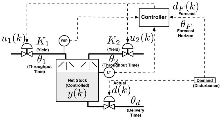
We noted in the Introduction that prior work has shown proof-of-concept and the benefits obtained from a control engineering approach (in general) and IMC and MPC (in particular) as decision frameworks for inventory management in supply chains [15], [22], [23], [24], [26], [36]. In this case study, we consider a supply chain management problem comprised of a production-inventory system with one inventory and two production nodes that requires a hybrid MPC solution. The production nodes consist of one primary factory and a secondary auxiliary one, as shown in Figure 7. Throughput time ${\theta }_1={\theta }_1^{\prime }+1$ and yield K₁ for the primary factory are 4 days and 0.9, respectively; for the auxiliary factory, the throughput time ${\theta }_2={\theta }_2^{\prime }+1$ and yield K₂ are 9 days and 0.8, respectively. Here we consider that the operating cost for the auxiliary factory is greater than the primary one because of the longer throughput time and lower yield. Therefore, this auxiliary production node should be accessed if and only if the primary node is running at its full capacity and unable to meet future market demand; likewise, production from the auxiliary node must be discontinued if future demand cannot justify its operation. The discrete decision of startup or shutdown of the auxiliary factory is a function of the continuous variables d_f (k) (demand forecast) and the work-in-progress (WIP) in the primary production node. Consequently, the system can be categorized as a hybrid system, where the inventory dynamics are governed by continuous variables (inventory, factory starts, demand and WIP) and a discrete decision (shut-down/start-up of the auxiliary factory). The dynamics of this system can be described using first principles model follows:

$$y(k+1)=y(k)+K_1{u}_1(k-{\theta }_1^{\prime })+K_2{u}_2(k-{\theta }_2^{\prime })-d(k)$$ (55)

$$\mathit{WIP}(k+1)=\sum _{i=0}^{{\theta }_1^{\prime }}{u}_1(k-i)$$ (56)

where d(k) = d_f (k − θ_f)+d_u(k) is the total customer demand comprising forecasted and unforecasted components, u₁(k) represents the starts for the primary production node, u₂(k) is the starts for the auxiliary production node, and WIP represents the work-in-progress in the primary production node. In order to ensure that the auxiliary factory is activated if and only if WIP in the primary factory is at its maximum capacity, we embed the following logical condition into the dynamical model:

$$u_2(k-{\theta }_2^{\prime })\ne 0\iff \mathit{WIP}(k+1)>{\mathit{Cap}}_{\mathit{max}}=600$$ (57)

Fig. 7.

Diagrammatical representation of a production-inventory system consisting of two production nodes (one primary, one secondary) and a single inventory examined in the supply chain management (SCM) case study.

The implication (⇔) in (57) can be converted into linear inequality constraints using Big-M constraints [40]. This conversion can be accomplished by introducing an auxiliary binary variable (δ) and an auxiliary continuous variable (z) followed by a MLD representation of (55)–(57) as in (1)–(3). In addition, we consider constraints on the process variables as follows:

$$0\le u_i(k)\le 200,i=1,2$$ (58)

$$0\le \mathit{WIP}(k)\le 600$$ (59)

$$0\le y(k)\le 1000$$ (60)

The MLD model of (55)–(57) and constraints (58)–(60) are then used to formulate an MPC problem of the form (29)–(30). The operational goal of this system is to meet the customer demand d(k) relying on production from the auxiliary factory only when necessary, while maintaining the net stock inventory level at a predefined setpoint. This can be accomplished by manipulating factory starts u₁(k), u₂(k) and feedforward compensation of forecasted demand d_f (k) simultaneously imposing the logical condition described in (57). Here we consider a sampling interval of T = 1 day, θ_f = p = 30 days.

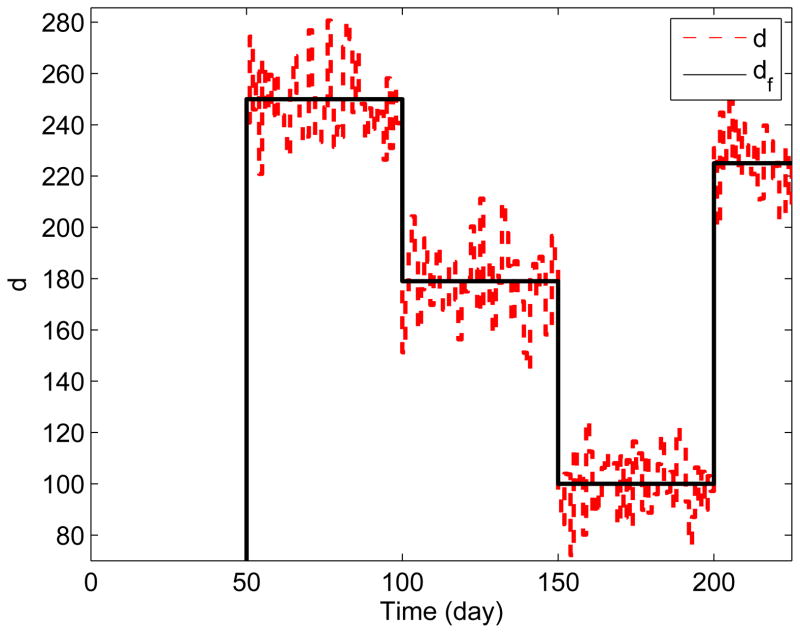
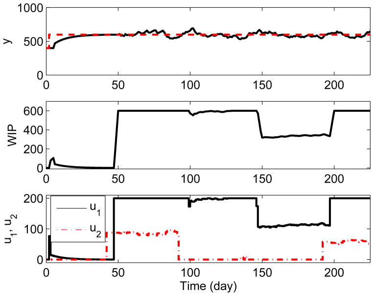
In practice, it is desirable to keep the factory starts as constant as possible (i.e., avoid factory “thrash”) while maintaining inventory at desired levels in the face of uncertain customer demand [26]. In order to examine the performance of the proposed multi-degree-of-freedom MPC formulation, we consider a piecewise stochastic customer demand signal and its forecast, which are shown in Figure 8. Figure 9 demonstrates the performance of the proposed formulation that uses multi-degree-of-freedom tuning parameters, α_r = 0.9, α_d = 0, f_a = 0.1, penalty weight parameters Q_y = 1, Q_Δu = diag{0 0}, Q_u = Q_d = Q_z = 0, prediction horizon p = 30 and control horizon m = 25. From the figure, it can be observed that the proposed MPC algorithm is able to satisfactorily maintain inventory at its predefined target, while producing little variation in the starts of the factories. Moreover, it is able to decide on the start-up/shutdown of the auxiliary factory in a desirable manner (i.e., by making minimal use of the auxiliary factory). This reduces operational cost while allowing the production system to meet customer demand without backorders.

Fig. 8.

Customer demand (red dashed line) and demand forecast (solid black line), SCM case study.

Fig. 9.

Response of net stock (y), work-in-progress (WIP), and factory starts (u₁,u₂) for the proposed multiple-degree-freedom formulation with tuning parameters: α_r = 0.9, α_d = 0, f_a = 0.1 and Q_y = 1, Q_Δu = diag{0 0}, Q_u = Q_d = Q_z = 0 for the demand in Figure 8.

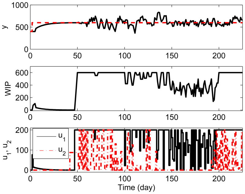
In order to assess the effectiveness of the proposed formulation, we compare its performance with the MPC formulation that relies on a constant plant-model mismatch over the prediction horizon. This formulation uses the move suppression weight (Q_Δu) in lieu of f_a to reduce the variation in the manipulated variables (i.e., starts) of the factories. Figure 10 presents the simulation results using Q_Δu = diag{0 0} while keeping all other parameters as in the previous case. The responses show evidence of very poor inventory control and very high variation in the starts of the factories as compared to the proposed formulation. To reduce the variation in the starts of the factories and verify the performance against the proposed formulation, we apply various values of the move suppression weight Q_Δu. Table II documents the maximum (peak) value of the inventory (y_max) and the closed-loop performance metrics J_e and J_Δu using the MPC formulation relying on a constant plant-model mismatch over the prediction horizon for five values of Q_Δu between 0 to 200. The last row of Table II documents these values for the three-degree-of-freedom (3-DoF) MPC formulation. The performance metrics J_e and J_Δu are measures of cumulative error (e = y − y_r) and variation in the rate-of-change of factory starts, respectively, which are given as follows:

$$J_e=\sum _{k=1}^{t/T_s}{(y(k)-y_r)}^T(y(k)-y_r)$$ (61)

$$J_{\mathrm{\Delta }u}=\sum _{k=1}^{t/T_s}{(u(k)-u(k-1))}^T(u(k)-u(k-1))$$ (62)

Fig. 10.

Response of net stock (y), Work-in-Progress (WIP), and factory starts (u₁,u₂) for the MPC formulation that relies on constant plant-model mismatch and move suppression tuning, with Q_Δu = diag{0 0} and Q_y = 1, Q_u = Q_d = Q_z = 0 for the demand in Figure 8.

TABLE II.

Closed-loop performance metrics J_Δu, J_e and maximum inventory (y_max) using mpc formulations relying on constant plant-model mismatch for various Q_Δu and a three-degree-of-freedom (3-dof) mpc formulation for f_a = 0.1.

Sl. No.	QΔu	JΔu	Je	ymax
1	diag{0 0}	267.9 × 104	13.15 × 105	834.63
2	diag{1 1}	94.67 × 104	11.15 × 105	763.865
3	diag{10 10}	25.82 × 104	10.69 × 105	809.24
4	diag{100 100}	4.81 × 104	12.71 × 105	890.94
5	diag{200 200}	3.038 × 104	15.71 × 105	939.24
6	3-DoF	8.345 × 104	4.426 × 105	692.76

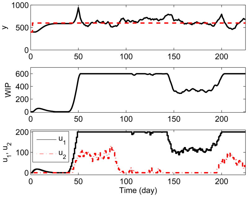
From Table II, it can be seen that the proposed 3-DoF formulation outperforms the constant plant-model mismatch based MPC formulation in terms of maximum peak in the inventory and J_e for all values of Q_Δu. On the other hand, increasing the move suppression weight Q_Δu lowers J_Δu, with the last two cases (i.e. Q_Δu = diag{100 100} and Q_Δu = diag{200 200}) yielding lower values of J_Δu than the 3-DoF MPC formulation. Comparing Figure 9 with Figure 11 shows that for the 3-DoF formulation, factory starts remain constant over a significant portion of the simulation, without leading to the substantial maximum inventory peak and corresponding demands on warehouse space resulting from Q_Δu = diag{200 200}. Thus, it can be concluded that the proposed 3 DoF-MPC algorithm can be useful for reducing overall operating costs and efficiently managing this form of hybrid production-inventory systems.

Fig. 11.

Response of net stock (y), Work-in-Progress (WIP), and factory starts (u₁,u₂) for the MPC formulation that relies on constant plant-model mismatch and move suppression tuning with Q_Δu = diag{200 200} and Q_y = 1, Q_u = Q_d = Q_z = 0 for the demand in Figure 8.

IV. Summary and Conclusions

Applications of hybrid systems are becoming increasingly common in many fields, yet many open challenges remain [10]. Adaptive behavioral interventions [17] and supply chain management [36] represent emerging application areas for control systems engineering that lie outside of the traditional industrial community, but that can be abstracted as hybrid production-inventory systems. Consequently, a control-oriented formulation for optimally managing these systems over time is relevant; this has been the primary focus of this paper.

To accomplish this goal, an improved MPC formulation for linear hybrid systems has been developed. The formulation relies on the MLD model representation that has been modified to include measured and the unmeasured disturbances that play an important role in these application domains. The controller formulation offers multiple-degree-of-freedom tuning parameters that enable the user to directly influence the speed of setpoint tracking and disturbance rejection (both measured and unmeasured) on each controlled variable; this tuning philosophy is intuitive in nature, amenable for achieving robustness, and has both fundamental and practical appeal. The applicability and efficiency of the proposed MPC formulation is demonstrated on a classical production-inventory problem example, a hypothetical adaptive behavioral intervention case study intended for improving parental function in homes of at-risk children, and a supply chain management (SCM) case study involving the need to systematically add (or remove) factory capacity in the face of varying external demand.

Simulation results in the adaptive intervention case study highlight the ability of the algorithm to be tuned to handle significant plant-model mismatch and disturbances while offering robust performance. The robustness properties of the algorithm are useful in the context of applying control engineering-based interventions to populations or cohort groups that may display wide participant variability in model parameters. In the SCM problem, the algorithm was useful in determining both the choice and magnitude of factory starts, while maintaining relatively uniform net stock inventory levels in the presence of drastic changes in market demand. The case study results showed that the proposed MPC scheme offered substantial performance and robustness benefits over a traditional MPC formulation with constant plant-model mismatch that uses move suppression weights to adjust the system response.

A formal robustness study lies beyond the scope of this paper, but represents a useful future addition to this body of work. Likewise, approaches that reduce the modeling effort required in practice and extend the functionality of the algorithm to nonlinear problems are particularly appropriate. Current efforts by the authors involve the development of controller formulations that are data-centric in nature; in this setting we are relying on the concept of model-on-demand (MoD) [41], [42], [43] and have developed a hybrid MoD-MPC approach that has been evaluated for adaptive behavioral interventions [44].

Appendix-A. COEFFICIENT MATRICES OF THE p-step AHEAD PREDICTIONS OF THE OUTPUT IN (13) AND CONSTRAINTS IN (14) AND (15)

$${\mathcal{H}}_1=\left[\begin{array}{ccccc}\mathcal{C}{\mathcal{B}}_1& 0& \cdots & 0& 0\\ \mathcal{C}\mathcal{A}{\mathcal{B}}_1-\mathcal{C}{\mathcal{B}}_1& \mathcal{C}{\mathcal{B}}_1& \cdots & 0& 0\\ \mathcal{C}{\mathcal{A}}^2{\mathcal{B}}_1-\mathcal{C}\mathcal{A}{\mathcal{B}}_1& \mathcal{C}\mathcal{A}{\mathcal{B}}_1-\mathcal{C}{\mathcal{B}}_1& \ddots & ⋮& ⋮\\ ⋮& ⋮& \ddots & \mathcal{C}{\mathcal{B}}_1& ⋮\\ \mathcal{C}{\mathcal{A}}^{m-1}{\mathcal{B}}_1-\mathcal{C}{\mathcal{A}}^{m-2}{\mathcal{B}}_1& \mathcal{C}{\mathcal{A}}^{m-2}{\mathcal{B}}_1-\mathcal{B}{\mathcal{A}}^{m-1}{\mathcal{B}}_1& \cdots & \mathcal{C}\mathcal{A}{\mathcal{B}}_1-\mathcal{C}{\mathcal{B}}_1& \mathcal{C}{\mathcal{B}}_1\\ \mathcal{C}{\mathcal{A}}^m{\mathcal{B}}_1-\mathcal{C}{\mathcal{A}}^{m-1}{\mathcal{B}}_1& \mathcal{C}{\mathcal{A}}^{m-1}{\mathcal{B}}_1-\mathcal{C}{\mathcal{A}}^{m-2}{\mathcal{B}}_1& \cdots & \mathcal{C}{\mathcal{A}}^2{\mathcal{B}}_1-\mathcal{C}\mathcal{A}{\mathcal{B}}_1& \mathcal{C}\mathcal{A}{\mathcal{B}}_1\\ ⋮& ⋮& ⋮& ⋮& ⋮\\ \mathcal{C}{\mathcal{A}}^{p-1}{\mathcal{B}}_1-\mathcal{C}{\mathcal{A}}^{p-2}{\mathcal{B}}_1& \mathcal{C}{\mathcal{A}}^{p-2}{\mathcal{B}}_1-\mathcal{C}{\mathcal{A}}^{p-1}{\mathcal{B}}_1& \cdots & \mathcal{C}{\mathcal{A}}^{p-m+1}{\mathcal{B}}_1-\mathcal{C}{\mathcal{A}}^{p-m}{\mathcal{B}}_1& \mathcal{C}{\mathcal{A}}^{p-m}{\mathcal{B}}_1\end{array}\right]$$ (A.1)

$${\mathcal{H}}_i=\left[\begin{array}{ccccc}\mathcal{C}{\mathcal{B}}_i& 0& \cdots & 0& 0\\ \mathcal{C}\mathcal{A}{\mathcal{B}}_i-\mathcal{C}{\mathcal{B}}_i& \mathcal{C}{\mathcal{B}}_i& \cdots & 0& 0\\ \mathcal{C}{\mathcal{A}}^2{\mathcal{B}}_i-\mathcal{C}\mathcal{A}{\mathcal{B}}_i& \mathcal{C}\mathcal{A}{\mathcal{B}}_i-\mathcal{C}{\mathcal{B}}_i& \cdots & ⋮& ⋮\\ ⋮& ⋮& \ddots & ⋮& ⋮\\ \mathcal{C}{\mathcal{A}}^{p-1}{\mathcal{B}}_i-\mathcal{C}{\mathcal{A}}^{p-2}{\mathcal{B}}_i& \mathcal{C}{\mathcal{A}}^{p-2}{\mathcal{B}}_i-\mathcal{C}{\mathcal{A}}^{p-3}{\mathcal{B}}_i& \cdots & \mathcal{C}\mathcal{A}{\mathcal{B}}_i-\mathcal{C}{\mathcal{B}}_i& \mathcal{C}{\mathcal{B}}_i\end{array}\right],i=2,3,d$$ (A.2)

$$\mathrm{\Phi }=\left[\begin{array}{c}\mathcal{C}\mathcal{A}\\ \mathcal{C}{\mathcal{A}}^2\\ ⋮\\ \mathcal{C}{\mathcal{A}}^p\end{array}\right]$$ (A.3)

$$H_{i1}=\left[\begin{array}{c}\mathcal{C}{\mathcal{B}}_i\\ \mathcal{C}\mathcal{A}{\mathcal{B}}_i\\ \mathcal{C}{\mathcal{A}}^2{\mathcal{B}}_i\\ ⋮\\ \mathcal{C}{\mathcal{A}}^{p-1}{\mathcal{B}}_i\end{array}\right]i=1,2,3,d$$ (A.4)

$${\overline{E}}_i=\text{diag}\{E_i,\cdots ,E_i\},i=2,3,d$$ (A.5)

$${\overline{E}}_4=\text{diag}\{-E_4,\cdots ,-E_4\}$$ (A.6)

$${\overline{E}}_5={[\begin{array}{cc}{E}_5& E_5\cdots E_5\end{array}]}^T$$ (A.7)

$${\overline{E}}_1=\left[\begin{array}{cccc}-E_1& 0& ·& 0\\ 0& \ddots & ·& ⋮\\ ⋮& \cdots & ·& -E_1\\ ⋮& ⋮& ⋮& ⋮\\ 0& \cdots & ·& -E_1\end{array}\right]$$ (A.8)

$${\mathcal{E}}_i=({\overline{E}}_4{\overline{\mathcal{H}}}_i+{\overline{E}}_i),i=1,2,3,d$$ (A.9)

$${\mathcal{E}}_4={\overline{E}}_4\overline{\mathrm{\Phi }}$$ (A.10)

$${\mathcal{E}}_{4i}={\overline{E}}_4{\overline{\mathcal{H}}}_{i1},i=1,2,3,d$$ (A.11)

$${\mathcal{E}}_5={\overline{E}}_5$$ (A.12)

$${\overline{\mathcal{H}}}_j=\left[\begin{array}{c}{[0]}_{n_y}\\ {\mathcal{H}}_j(1:(p-1)n_y,:)\end{array}\right]j=1,2,3,d,11,21,31,d1$$ (A.13)

$$\overline{\mathrm{\Phi }}=\left[\begin{array}{c}\mathcal{C}\\ \mathrm{\Phi }(1:(p-1)n_y,:)\end{array}\right]$$ (A.14)

Here n_y is number of outputs, [0]_ny denotes matrix with n_y rows that has all the elements 0 and *(1: (p−1)n_y, :) should be read as row 1 to row (p − 1)n_y of the matrix * with all the columns.

Appendix-B. COEFFICIENT MATRICES OF THE OBJECTIVE FUNCTION IN (29) AND CONSTRAINTS IN (30) OF THE MPC PROBLEM

$$\mathcal{H}=2\left[\begin{array}{ccc}{{\mathcal{H}}_1}^T{\widehat{Q}}_y{\mathcal{H}}_1+{\widehat{Q}}_{\mathrm{\Delta }u}+{\widehat{Q}}_u& {{\mathcal{H}}_1}^T{\widehat{Q}}_y{\mathcal{H}}_2& {{\mathcal{H}}_1}^T{\widehat{Q}}_y{\mathcal{H}}_3\\ {{\mathcal{H}}_2}^T{\widehat{Q}}_y{\mathcal{H}}_1& {{\mathcal{H}}_2}^T{\widehat{Q}}_y{\mathcal{H}}_2+{\widehat{Q}}_d& {{\mathcal{H}}_2}^T{\widehat{Q}}_y{\mathcal{H}}_3\\ {{\mathcal{H}}_3}^T{\widehat{Q}}_y{\mathcal{H}}_1& {{\mathcal{H}}_3}^T{\widehat{Q}}_y{\mathcal{H}}_2& {{\mathcal{H}}_3}^T{\widehat{Q}}_y{\mathcal{H}}_3+{\widehat{Q}}_z\end{array}\right]$$ (B.1)

$$\mathcal{G}=2{[\begin{array}{ccc}{g}_1& g_2& g_3\end{array}]}^T$$ (B.2)

where,

$$\begin{array}{l}{g}_1=X{(k)}^T{\mathrm{\Phi }}^T{\widehat{Q}}_y{\mathcal{H}}_1-{{\mathcal{Y}}_r}^T{\widehat{Q}}_y{\mathcal{H}}_1-{{\mathcal{U}}_r}^T{\widehat{Q}}_u+\\ \mathcal{D}{(k)}^T{{\mathcal{H}}_d}^T{\widehat{Q}}_y{\mathcal{H}}_1-u{(k-1)}^T({R_{u0}}^T\widehat{Q_{\mathrm{\Delta }u}}{R}_u+{H_{11}}^T{\widehat{Q}}_y{\mathcal{H}}_1)-\\ \delta {(k-1)}^T{H_{21}}^T{\widehat{Q}}_y{\mathcal{H}}_1-z{(k-1)}^T{H_{31}}^T{\widehat{Q}}_y{\mathcal{H}}_1-d_{\mathit{flt}}{(k-1)}^T{H_{d1}}^T{\widehat{Q}}_y{\mathcal{H}}_1\\ g_2=X{(k)}^T{\mathrm{\Phi }}^T{\widehat{Q}}_y{\mathcal{H}}_2-{{\mathcal{Y}}_r}^T{\widehat{Q}}_y{\mathcal{H}}_2-{\overline{\delta }}_r^T{\widehat{Q}}_d+\mathcal{D}{(k)}^T{{\mathcal{H}}_d}^T{\widehat{Q}}_y{\mathcal{H}}_2-u{(k-1)}^T{H_{11}}^T{\widehat{Q}}_y{H}_2-\\ \delta {(k-1)}^T{H_{21}}^T{\widehat{Q}}_y{\mathcal{H}}_2-z{(k-1)}^T{H_{31}}^T{\widehat{Q}}_y{\mathcal{H}}_2-d_{\mathit{flt}}{(k-1)}^T{H_{d1}}^T{\widehat{Q}}_y{\mathcal{H}}_2\\ g_3=X{(k)}^T{\mathrm{\Phi }}^T{\widehat{Q}}_y{\mathcal{H}}_3-{{\mathcal{Y}}_r}^T{\widehat{Q}}_y{\mathcal{H}}_3-{{\mathcal{Z}}_r}^T{\widehat{Q}}_z+\mathcal{D}{(k)}^T{{\mathcal{H}}_d}^T{\widehat{Q}}_y{\mathcal{H}}_3-u{(k-1)}^T{H_{11}}^T{\widehat{Q}}_y{\mathcal{H}}_3-\\ \delta {(k-1)}^T{H_{21}}^T{\widehat{Q}}_y{\mathcal{H}}_3-z{(k-1)}^T{H_{31}}^T{\widehat{Q}}_y{\mathcal{H}}_3-d_{\mathit{flt}}{(k-1)}^T{H_{d1}}^T{\widehat{Q}}_y{\mathcal{H}}_3\\ \mathcal{S}=\left[\begin{array}{c}{s}_1\\ s_2\\ -s_2\end{array}\right]\end{array}$$ (B.3)

where

$$\begin{array}{l}{s}_1=[\begin{array}{ccc}{\mathcal{E}}_1& {\mathcal{E}}_2& {\mathcal{E}}_3\end{array}];s_2=\left[\begin{array}{ccc}{\mathcal{H}}_1& {\mathcal{H}}_2& {\mathcal{H}}_3\\ I_{m(nu)}& {[0]}_{m(nu)\times p(nd)}& {[0]}_{m(nu)\times p(nz)}\\ R_u& {[0]}_{m(nu)\times p(nd)}& {[0]}_{m(nu)\times p(nz)}\end{array}\right]\\ b=\left[\begin{array}{c}{\mathcal{E}}_5-{\mathcal{E}}_{4}X(k)-{\mathcal{E}}_d\mathcal{D}(k)+{\mathcal{E}}_{41}u(k-1)+{\mathcal{E}}_{42}\delta (k-1)+{\mathcal{E}}_{43}z(k-1)+{\mathcal{E}}_{4d}{d}_{\mathit{flt}}(k-1)\\ {\mathcal{Y}}_{max}-\mathrm{\Phi }X(k)-H_d\mathcal{D}(k)+H_{11}u(k-1)+H_{21}\delta (k-1)+H_{31}z(k-1)+H_{d1}{d}_{\mathit{flt}}(k-1)\\ {\mathcal{U}}_{max}\\ \mathrm{\Delta }{\mathcal{U}}_{max}+R_{u0}u(k-1)\\ -{\mathcal{Y}}_{min}+\mathrm{\Phi }X(k)+H_d\mathcal{D}(k)-H_{11}u(k-1)-H_{21}\delta (k-1)-H_{31}z(k-1)-H_{d1}{d}_{\mathit{flt}}(k-1)\\ -{\mathcal{U}}_{min}\\ -\mathrm{\Delta }{\mathcal{U}}_{min}-R_{u0}u(k-1)\end{array}\right]\end{array}$$ (B.4)

Here n_u, n_d and n_z are dimensions of the inputs, the auxiliary binary variables δ and the auxiliary continuous variables z, respectively.

References

- 1.Bemporad A, Morari M. Control of systems integrating logic, dynamics, and constraints. Automatica. 1999;35(3):407–427. [Google Scholar]
- 2.Nandola NN, Bhartiya S. A multiple model approach for predictive control of nonlinear hybrid systems. J Process Control. 2008;18(2):131–148. [Google Scholar]
- 3.Nandola NN, Bhartiya S. Hybrid system identification using a structural approach and its model based control: An experimental validation. Nonlinear Anal Hybrid Syst. 2009;3(2):87–100. [Google Scholar]
- 4.Roll J, Bemporad A, Ljung L. Identification of piecewise affine systems via mixed-integer programming. Automatica. 2004;40(1):37–50. [Google Scholar]
- 5.Branicky MS, Borkar VS, Mitter SK. A unified framework for hybrid control: model and optimal control theory. IEEE Trans Autom Control. 1998;43(1):31–45. [Google Scholar]
- 6.Nandola NN, Bhartiya S. A computationally efficient scheme for model predictive control of nonlinear hybrid systems using generalized outer approximation. Ind Eng Chem Res. 2009;48(12):5767–5778. [Google Scholar]
- 7.Prakash J, Patwardhan SC, Shah SL. State estimation ad nonlinear predictive control of autonomous hybrid system using derivative free state estimators. Journal of Process Control. 2010;20(7):787–799. [Google Scholar]
- 8.Lee CK, Singer AB, Barton PI. Global optimization of linear hybrid systems with explicit transitions. Systems & Control Letters. 2004;51(5):363–375. [Google Scholar]
- 9.Till J, Engell S, Panek S, Stursberg O. Applied hybrid system optimization: An empirical investigation of complexity. Control Engineering Practice. 2004;12(10):1291–1303. [Google Scholar]
- 10.Camacho EF, Ramirez DR, Limon D, Munoz de la Peña D, Alamo T. Model predictive control techniques for hybrid systems. Annual Reviews in Control. 2010;34:21–31. [Google Scholar]
- 11.Grubbström RW, Wikner J. Inventory trigger control policies developed in terms of control theory. International Journal of Production Economics. 1996;45:397–406. [Google Scholar]
- 12.Riddalls CE, Bennett S. Production-inventory system controller design and supply chain dynamics. International Journal of Systems Science. 2002;33(3):181–195. [Google Scholar]
- 13.Ortega M, Lin L. Control theory applications to the production-inventory problem: a review. International Journal of Production Research. 2004;42(11):2303–2322. [Google Scholar]
- 14.Sarimveis H, Patrinos P, Tarantilis CD, Kiranoudis CT. Dynamic modeling and control of supply chain systems: A review. Computers & Operations Research. 2008;35:3530–3561. [Google Scholar]
- 15.Schwartz JD, Rivera DE. A process control approach to tactical inventory management in production-inventory systems. International Journal of Production Economics. 2010;125(1):111–124. [Google Scholar]
- 16.Collins LM, Murphy SA, Bierman KL. A conceptual framework for adaptive preventive interventions. Prevention Science. 2004;5(3):185–196. doi: 10.1023/b:prev.0000037641.26017.00. [DOI] [PMC free article] [PubMed] [Google Scholar]
- 17.Rivera DE, Pew MD, Collins LM. Using engineering control principles to inform the design of adaptive interventions a conceptual introduction. Drug and Alcohol Dependence. 2007;88(2):S31–S40. doi: 10.1016/j.drugalcdep.2006.10.020. [DOI] [PMC free article] [PubMed] [Google Scholar]
- 18.Navarro-Barrientos JE, Rivera DE, Collins LM. A dynamical model for describing behavioural interventions for weight and body composition change. Mathematical and Computer Modelling of Dynamical Systems. 2011 Apr;17(2):183–203. doi: 10.1080/13873954.2010.520409. [DOI] [PMC free article] [PubMed] [Google Scholar]
- 19.Riley WT, Rivera DE, Atienza AA, Nilsen W, Allison SM, Mermelstein R. Health behavior models in the age of mobile interventions: are our theories up to the task? Translational Behavioral Medicine. 2011 Mar;1(1):53–71. doi: 10.1007/s13142-011-0021-7. [DOI] [PMC free article] [PubMed] [Google Scholar]
- 20.Zafra-Cabeza A, Rivera DE, Collins LM, Ridao MA, Camacho EF. A risk-based Model Predictive Control approach to adaptive behavioral interventions in behavioral health. IEEE Transactions in Control Systems Technology. 2011 Jun;19(4):891–901. doi: 10.1109/TCST.2010.2052256. [DOI] [PMC free article] [PubMed] [Google Scholar]
- 21.Silver EA, Pyke DF, Petersen R. Inventory Management and Production Planning and Scheduling. 3. Wiley; Upper Saddle River, NJ: 1998. [Google Scholar]
- 22.Rivera DE, Pew MD. Evaluating PID control for supply chain management: a freshman design project. 44th IEEE Conference on Decision and Control and 2005 European Control Conference; Seville, Spain. December 2005.pp. 3415–3419. [Google Scholar]
- 23.Schwartz JD. PhD thesis. Arizona State University; USA: 2008. Next generation supply chain management: control, optimization, and system identification. [Google Scholar]
- 24.Schwartz JD, Arahal MR, Rivera DE, Smith KD. Control-relevant demand forecasting for tactical decision-making in semiconductor manufacturing supply chain management. IEEE Transactions on Semiconductor Manufacturing. 2009 Feb;22(1):154–163. [Google Scholar]
- 25.Dejonckheere J, Disney SM, Lambrecht MR, Towill DR. Measuring and avoiding the bullwhip effect: a control theoretic approach. European Journal of Operational Research. 2003;147:567–590. [Google Scholar]
- 26.Wang W, Rivera DE. Model predictive control for tactical decision-making in semiconductor manufacturing supply chain management. IEEE Trans Control Syst Technol. 2008 Sep;16(5):841–855. [Google Scholar]
- 27.Lee JH, Morari M, García CE. State-space interpretation of model predictive control. Automatica. 1994;30(4):707–717. [Google Scholar]
- 28.Lee JH, Yu ZH. Tuning of model predictive controllers for robust performance. Comput Chem Eng. 1994;18(1):15–37. [Google Scholar]
- 29.Nandola NN, Rivera DE. A novel model predictive control formulation for hybrid systems with application to adaptive behavioral interventions. ACC; Baltimore, Maryland, USA. June 30–July 02 2010; pp. 6286–6292. [DOI] [PMC free article] [PubMed] [Google Scholar]
- 30.Camacho EF, Bordons C. Model predictive control. 2. Springer-Verlag; 2004. [Google Scholar]
- 31.Prett DM, García . Butterworths Series in Chemical Engineering. Butterworths publishers; 1988. Fundamental Process Control. [Google Scholar]
- 32.Williams HP. Model building in mathematical programming. John Wiley & Sons; New York: 1993. [Google Scholar]
- 33.Morari M, Zafiriou E. Robust Process Control. Englewood Cliffs, NJ: Prentice-Hall; 1989. [Google Scholar]
- 34.Dua V, Bozinis NA, Pistikopoulos EN. A multiparametric programming approach for mixed-integer quadratic engineering problems. Computers & Chemical Engineering. 2002;26(4–5):715–733. [Google Scholar]
- 35.Garriga JL, Soroush M. Model predictive control tuning methods: a review. Ind Eng Chem Res. 2010;49:3505–3515. [Google Scholar]
- 36.Schwartz JD, Wang W, Rivera DE. Simulation-based optimization of process control policies for inventory management in supply chains. Automatica. 2006;42(8):1311–1320. [Google Scholar]
- 37.Zhou K, Doyle JC, Glover K. Robust and Optimal Control. PTR Prentice Hall; New Jersey: 1996. [Google Scholar]
- 38.Rossiter JA. Model-based predictive control: A practical approach. CRC Press; Boca Raton, FL: 2003. [Google Scholar]
- 39.Conduct Problems Prevention Research Group. A developmental and clinical model for the prevention of conduct disorders: The Fast Track program. Development and Psychopathology. 1992;4:509–528. [Google Scholar]
- 40.Raman R, Grossmann IE. Relation between MILP modelling and logical inference for chemical process synthesis. Comput Chem Eng. 1991;15(2):73–84. [Google Scholar]
- 41.Braun MW, Rivera DE, Stenman A. A model-on-demand identification methodology for nonlinear process systems. Int J Control. 2001;74(18):1708–1717. [Google Scholar]
- 42.Stenman A. PhD thesis. Linköping University; Sweden: 1999. Model-on-demand: Algorithms, analysis and applications. [Google Scholar]
- 43.Braun MW. PhD thesis. Arizona State University; USA: 2001. Model-on-demand nonlinear estimation and model predictive control: Novel methodologies for process control and supply chain management. [Google Scholar]
- 44.Nandola NN, Rivera DE. Model-on-demand predictive control for nonlinear hybrid systems with application to adaptive behavioral interventions. 49th IEEE Conference on Decision and Control; Atlanta, Georgia. December 2010; pp. 6113–6118. [DOI] [PMC free article] [PubMed] [Google Scholar]