WHEN DOES IMPROVING HEALTH RAISE GDP?

Abstract

We assess quantitatively the effect of exogenous health improvements on output per capita. Our simulation model allows for a direct effect of health on worker productivity, as well as indirect effects that run through schooling, the size and age-structure of the population, capital accumulation, and crowding of fixed natural resources. The model is parameterized using a combination of microeconomic estimates, data on demographics, disease burdens, and natural resource income in developing countries, and standard components of quantitative macroeconomic theory. We consider both changes in general health, proxied by improvements in life expectancy, and changes in the prevalence of two particular diseases: malaria and tuberculosis. We find that the effects of health improvements on income per capita are substantially lower than those that are often quoted by policy-makers, and may not emerge at all for three decades or more after the initial improvement in health. The results suggest that proponents of efforts to improve health in developing countries should rely on humanitarian rather than economic arguments.

1 Introduction

Chronic ill-health and the prospect of premature mortality haunt billions of people around the developing world. Few goals can be more worthy than that of ameliorating these burdens. Today, there exists a widespread belief that significant improvements in health are within reach of affordable policy interventions, whether led by governments or by large-scale philanthropies. There also exists a widespread consensus that improving the health of people in poor countries will lead to significant economic gains. The prospect of such economic benefits is often cited as an important secondary justification for health initiatives. For example, the report of the Commission on Macroeconomics and Health (2001), chaired by Jeffrey Sachs, finds evidence that health is one of the most important determinants of a country’s economic success. Similarly, the Abuja Declaration of 2005, signed by fifty three African heads of state, notes that “malaria has slowed economic growth in African countries by 1.3% per year as a result of which GDP for African countries is now 37% lower than it would have been in the absence of malaria.”¹

In this paper we assess the claim that improvements in health lead to increases in economic growth. Our findings are not supportive of the popularly held view. We find that large improvements in health lead, in the long run, to modest increases in GDP per capita. Further, these increases in GDP per capita take several decades to arrive. Controlling specific diseases that have a high burden in developing countries would also produce small effects. For example, we find that the effect of eradicating malaria in a typical sub-Saharan country would be to raise GDP per capita by only about two percent in the long run. Our evidence thus suggests that proponents of efforts to improve health in developing countries should rely on humanitarian rather than economic arguments.

Existing research on the effects of health on economic outcomes uses data at both the microeconomic (household) and macroeconomic (country) level. Microeconomists have found extensive evidence that an individual’s health is an important determinant of his or her economic performance. Various measures of poor health, including malnutrition, anemia, and exposure to disease in utero and during childhood, have all been shown to have a negative effect on a person’s wages or productivity. At the macroeconomic level, there is a strong positive correlation between income per capita and life expectancy or other measures of health. Thus there is a prima facie case for believing that health improvements will make a country richer.

Drawing a macroeconomic conclusion directly from either the microeconomic evidence or the cross-sectional correlation is problematic, however. Outcomes of microeconomic studies are often measured in units that do not map immediately into macroeconomic effects. More importantly, microeconomic studies are unable to control for general equilibrium effects of changes in population health. For example, an increase in life expectancy may lead to a larger population, in turn reducing available resources per capita and possibly undoing the economic benefits of better health. On the other hand, macroeconomic cross-country regressions that could potentially capture these effects typically suffer from omitted variables bias and reverse causation problems. In an important recent study, Acemoglu and Johnson (2007) conclude that, when the problems of health’s endogeneity and omitted variables are corrected, health improvements in the period after World War II actually had a negative effect on income per capita.

Our goal in this paper is to answer the macroeconomic question of how much national income can be raised by exogenous health improvements by building up from microeconomic estimates, using a simulation model. Our model requires the specification of three sets of functional relationships and parameters: those involving the effect of health on labor productivity and other aspects of human capital; those involving the demographic response to health and mortality changes; and those involving the aggregate production function. Relative to reduced-form econometrics, our methodology is well suited to highlighting the causal mechanisms behind changes in output per capita, and therefore by implication which sets of policies or behavioral variables are likely to have a quantitatively significant effect on the relationship between health and income.

We apply the model to two distinct types of exogenous changes in health. The first is an increase in life expectancy, treating life expectancy as a summary measure of the general state of health in a nation. In particular, we consider the effect of exogenously raising life expectancy at birth from 40 to 60 years. This approximately corresponds with the most dramatic improvement in health observed during the international epidemiological transition studied by Acemoglu and Johnson. The key finding from these simulations is that even large increases in life expectancy, which could raise per capita income in the long run by around 15 percent, may reduce income by up to 5 percent for 30–40 years or more after the shock.

The second type of change in health we consider is the eradication of particular diseases. Our results focus on two infectious diseases that are particularly prevalent in the developing world: malaria and tuberculosis. These simulations have two key results. The first is that, for either of the diseases considered, even complete eradication has a relatively small impact on income per capita in either the short or the long run, not exceeding a few percentage points. The second is that these relatively small effects vary by disease. For example, in the short run, eradicating tuberculosis raises income per capita whereas eradicating malaria lowers it. The different effects on income of eradicating these diseases arise largely because tuberculosis strikes mostly prime-age workers, while malaria affects mainly young children.

The simulation-based methodology allows us to take into account both general equilibrium effects and the dynamic effect of health through channels including the evolution of the size and age-structure of the population, capital accumulation, and resource crowding. The analysis is well adapted to considering the dynamic path of the economy over the course of this evolution, rather than merely comparing steady states, and to providing a quantitative characterization of this evolution in the face of particular interventions. The simulation approach also permits analysis of the strength of the various mechanisms at work. For instance, it is straightforward to examine the sensitivity of the results to different estimates of the effect of disease on effective labor supply or the speed of the demographic transition.

Our exercise should not be mistaken for an analysis of the welfare impacts of health improvements. The primary benefits from health improvements are in terms of lives saved and suffering avoided. The issue we study – whether there are also effects on income per capita – is of minor importance in welfare terms. Similarly, while it might be interesting to ask whether health improvements of the sort that we study could be “self-financing,” we do not go down this path. Among other things, we do not have any estimate of the cost of the health improvements we consider, nor do we specify who (government, households, etc.) are paying for them.

A more profitable use of the analysis, in our view, is to suggest policies that are complementary to health improvements in terms of raising income per capita. We see three areas where this is particularly relevant. First, we find that health improvements can result in large population increases that can have a significant negative effect on income per capita over an extended period. Providing women with sufficient knowledge of, and access to, a range of family-planning options may ameliorate this effect. Second, one important channel through which population increases reduce income per capita is capital shallowing. Therefore policies and institutions that enable a sizable and sustained current account deficit without incurring unduly high interest burdens, are likely to be particularly important following an increase in life expectancy. Finally, many or most health interventions have the largest effect on infant mortality, and therefore are likely to lead to a substantial increase in the number of children. Since increased human capital formation is likely to be optimal following an improvement in health, and is an important factor offsetting population pressure, it is particularly important to ensure an adequate supply of teachers and school facilities in the years following public health improvements.

The rest of this paper is structured as follows. Section Two presents the model and discusses our choice of base case parameters. Section Three presents simulation results for the base case model, and then discusses the sensitivity of results to altering our parameter assumptions. In Section Four, we consider the eradication of two specific diseases: malaria and tuberculosis. We discuss how the model has to be altered and present simulation results. Section Five concludes.

2 The Model and its Parameterization

Health affects income through a number of channels, and the dynamics of these effects can be stretched out over several decades. Thus, analyzing the effect of a health intervention entails comparing the complete paths of income and other endogenous variables in the scenario in which the intervention takes place to an alternative in which it does not. Similarly, alternative parameter assumptions regarding the different components of the model will yield different dynamic paths of all the endogenous variables.

We consider two different sorts of health interventions. First, we consider a “general” health improvement. Specifically, we consider a shift in life expectancy at birth from e₀ = 40 to e₀ = 60 using a model life table. Second, we consider the eradication of two specific diseases: malaria and tuberculosis.

The model features both demographic and economic elements. The demographic elements comprise estimates of mortality and fertility by age. The economic elements include the specification of the aggregate production function and the specification of the response of variables such as human capital to changes in health. We consider each element in turn.

2.1 Demographic Structure

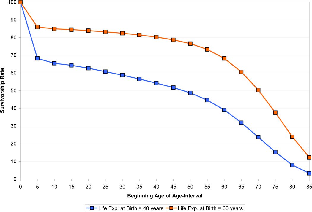
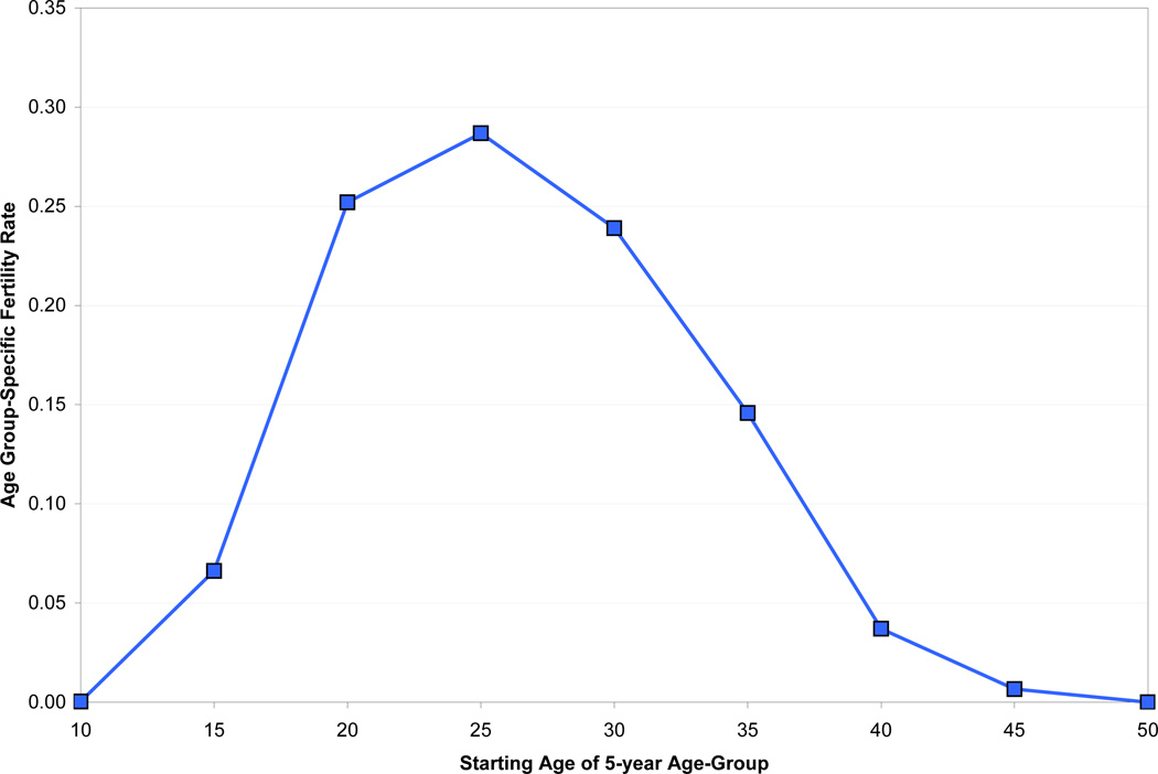
The demographic part of the model takes age-specific mortality and fertility schedules as inputs. Figures 1 and 2 show the data that we use for analyzing a general health improvement. Figure 1 shows the probability of survival to different ages at life expectancies of 40 (before the health improvement) and 60 (after the improvement), using the female model life table for the South Asia region from the United Nations (1982).² Figure 2 shows age-specific fertility data for Sri Lanka in 1953 from Keyfitz and Flieger (1968), which we take as a measure of fertility before the general health improvement. These data are among the earliest available and should capture much of the relevant demographic behavior over the period considered by Acemoglu and Johnson (2007). In practice, population is divided into 5-year age groups, and each time period in our model corresponds to five years.

Figure 1.

Survivorship Functions, UN Model Life Table, South Asia

Figure 2.

Fertility Schedule, Sri Lanka, 1953

We assume that prior to the health improvement, fertility and mortality rates have been constant for long enough that the population is stable (that is, the relative sizes of different age groups are constant as is the growth rate of the population). The health improvement switches the country immediately to the new mortality schedule.³ A critical component of the model is what happens to fertility rates when mortality changes. We assume that in the long run, fertility adjusts proportionally at each age such that the growth rate of the population eventually returns to its pre-shock level. We further assume that the adjustment in age-specific fertility occurs in a linear fashion over some transition period.

Estimates of the appropriate length of this fertility transition period are difficult to come by. We assume as a base case a transition period of 50 years. This fertility adjustment is a little slower than some accounts of the East Asian demographic transition, which suggest a period of about 25–30 years, but seems quite consistent with evidence from Europe and India and perhaps even a little optimistic in Africa (see Lee et al. (2001) for a brief summary of the evidence). Below we test the sensitivity of our results to different assumptions regarding the length of the transition period. When we consider the eradication of a specific diseases in Section Four, we use a table of age-specific deaths from that disease to create a cause-deleted mortality schedule and make similar assumptions about the response of fertility to mortality decline.

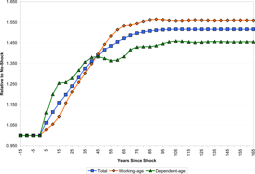
Figure 3 shows the sizes of the overall population and of the working-age and dependent-age segments of the population, all relative to the baseline in which no improvement in health takes place. Population in the health improvement scenario stabilizes at roughly 1.5 times the size of the baseline (note that population is growing at an annual rate of 1.5 percent in the baseline case; growth reaches 2.5 percent in the decade following the health improvement). Because of demographic momentum, this stabilization takes longer than the 50 years that we assume it takes fertility to adjust. For the first 40 years of the transition, the ratio of dependents to working-age adults is higher in the health improvement scenario than in the baseline. This effect peaks about 15 years after the shock, at which time the dependency ratio has increased by about 0.10, from about 0.69 to about 0.79. Thereafter, the dependency ratio gradually declines to a long-run level of about 0.64. In the long run, therefore, there is a demographic dividend in terms of income per capita from the decline in mortality, but this only occurs more than half a century after the shock.

Figure 3.

Effect of the Life Expectancy Shock on Population Size

2.2 Production and Physical Capital Accumulation

In our base case model, aggregate production is given by a standard Cobb-Douglas production function. The factor inputs are land (which we use as a shorthand for all fixed factors of production), capital, and human capital, so that aggregate output in period t, Y_t, is:

$$Y_t=A_t{K}_t^{\alpha }{H}_t^{\beta }{X}^{1-\alpha -\beta }$$

where α + β ≤ 1, X is a fixed arbitrary stock of land and A_t is productivity.

We assume fairly standard values for factor shares: we set α = 0.3 and β = 0.6, meaning that the implied share of land is 10 percent. In a later section we revisit the role of fixed factors of production. We consider the sensitivity of our results to both the share of land in national income and the elasticity of substitution between land and other factors of production. We also examine data on natural resource shares of national income.

Productivity grows at an exogenous rate that does not respond to any of the changes in the model. For convenience, the growth rate is set to equal the steady-state rate of population growth times the share of land, so that income per capita is constant in the steady state. Because all of our results entail a comparison of income in the case of a health intervention to the case where no intervention takes place, the underlying rate of technological change is of very little importance.

We handle capital accumulation extremely simply, by making the Solovian assumption that a fixed share of national income is saved in each period.⁴ Accordingly, the stock of capital in period t, K_t, evolves over time according to:

$$K_{t+1}=s{Y}_t+(1-\delta )K_t,$$

where s and δ are the fixed saving and depreciation rates, respectively. We assume that the annual savings rate is 10 percent, which is close to the average for countries in sub-Saharan Africa, and assign a standard value to the depreciation rate of five percent. Below we also consider the case of an economy open to international capital flows.

2.3 Human Capital

We model an individual’s human capital as a function of his or her schooling, experience, and health. We assume that human capital inputs of individuals with different characteristics are perfectly substitutable. Thus the stock of human capital in period t, H_t, is:

$$H_t=\sum _{15\le i\le 65}(h_{i,t}^h\times h_{i,t}^s\times h_{i,t}^e)N_{i,t},$$

where N_i,t is the number of individuals of age i in the population in period t. We assume that children enter the labor force at 15 and workers leave the labor force at 65.

Our treatment of schooling and experience is standard. Years of schooling are aggregated into human capital from schooling using the piecewise log-linear specification:

$$h_{i,t}^s=\{\begin{array}{ccc}\hfill \text{exp}[{\theta }_{1}S]\hfill & \hfill \text{if}\hfill & \hfill S\le 4\hfill \\ \hfill \text{exp}[4{\theta }_1+{\theta }_2(S-4)]\hfill & \hfill \text{if}\hfill & \hfill 4<S\le 8\hfill \\ \hfill \text{exp}[4{\theta }_1+4{\theta }_2+{\theta }_3(S-8)]\hfill & \hfill \text{if}\hfill & \hfill S>8\hfill \end{array}$$

where we use values of θ₁ = 0.134, θ₂ = 0.101, and θ₃ = 0.068, based on Hall and Jones (1999). The return to schooling will be relevant for the exercises we conduct because improvements in health will raise the average level of schooling.

Human capital from on-the-job experience for a worker of age i in any period t, $h_{i,t}^e$, is computed as:

$$h_{i,t}^e=\text{exp}[\varphi (i-15)+\psi {(i-15)}^2]$$

where, based on Bils and Klenow (2000), who provide an estimate of the average return to experience in a sample of 48 countries, we use a ϕ value of 0.0495 and a value of −0.0007 for ψ. Experience will play a role in our simulations because declines in mortality and fertility will lead to a population with higher average age and thus higher average experience.

2.3.1 Human Capital from Health

We use two different methods for parameterizing the effects of a general health improvement (that is, an increase in life expectancy at birth from 40 to 60) on human capital.

The first method for modeling the effect of a general improvement in health uses the estimate of the effect of increased adult survival rates (ASR) on productivity generated in Weil (2007), which in turn draws on a large number of well-identified microeconomic studies. The ASR is defined as the probability that an individual will attain the age of 60, conditional on having attained the age of 15 using the current life table. Weil estimates the structural coefficient linking the log of human capital in the form of health to ASR as 0.653. To give a concrete example of the size of this effect, a change in life expectancy at birth from 40 to 60 corresponds, using the UN female model life table for the South Asia region, to a change in the ASR from 0.50 to 0.72. Applying the coefficient above implies an increase of 15 percent in health human capital per worker.

The second method of capturing the direct effect of health improvements on productivity relies on the ratings of disease incidence and severity that are used to construct estimates of years lost due to disability (YLD) around the world by the World Health Organization (WHO). The WHO provides a general measure of YLDs and then also measures disease-specific YLDs, both broken down by age group. A country’s YLD for a given disease is constructed as:

$$YLD=I\times DW\times L$$

where I is the number of incident (newly-arising) cases in a period, DW is the disability weight attached to the disease, and L is the average duration of the disease until remission or death. The crucial parameter here is the disability weight, which is intended to be a cardinal measure of the severity of different diseases or impairments, on a scale from 0, indicating perfect health, to 1, indicating death. Disability weights are constructed by panels of healthcare providers and medical experts using a “person trade-off” protocol which establishes utility equivalences between years of life lived in different states of health. One year lived with a disability provides the same utility as (1 – DW) years lived disability-free (Murray, 1996). Disability weights are therefore not primarily intended as a measure of labor supply. Nevertheless, these estimates provide at least some basis for comparing the effects of different diseases, as well as a cross-check on the results using the ASR parameter discussed earlier.⁵

Because YLD data play a significant role in the analysis below, it is worth exploring these data in more detail. Table 1 shows data from the WHO “AFRO E” region, (defined as Africa with high child and very high adult mortality). We look at per capita YLDs for men in the 30–44 age group and boys aged 0–4. Overall, the men average 13.5 percent of a YLD per capita per year, with one-third of this burden coming from infectious and parasitic diseases. HIV/AIDS makes up half of the infectious disease burden, while the two diseases that we consider below make relatively small contributions. Tuberculosis accounts for 0.005 YLDs, or 3.5 percent of the disability burden, while malaria accounts for only 0.001 YLDs, or 1 percent of the total disability burden. The boys average 16.6 percent of a YLD per capita per year, with two thirds of the burden coming from infectious diseases.

Table 1.

Per Capita YLDs for Males, AFRO E Region

	Ages 0–4	Ages 30–44
All Causes	0.1662	0.1352
Communicable, Maternal, Perinatal and Nutritional Conditions	0.1084	0.0406
Infectious and Parasitic Diseases	0.0432	0.0397
Tuberculosis	0.0003	0.0046
HIV/AIDS	0.0002	0.0206
Malaria	0.0251	0.0014
Non-communicable Diseases	0.0450	0.0717
Injuries	0.0129	0.0228

Source: WHO, Global Burden of Disease (2002) Revised Estimates

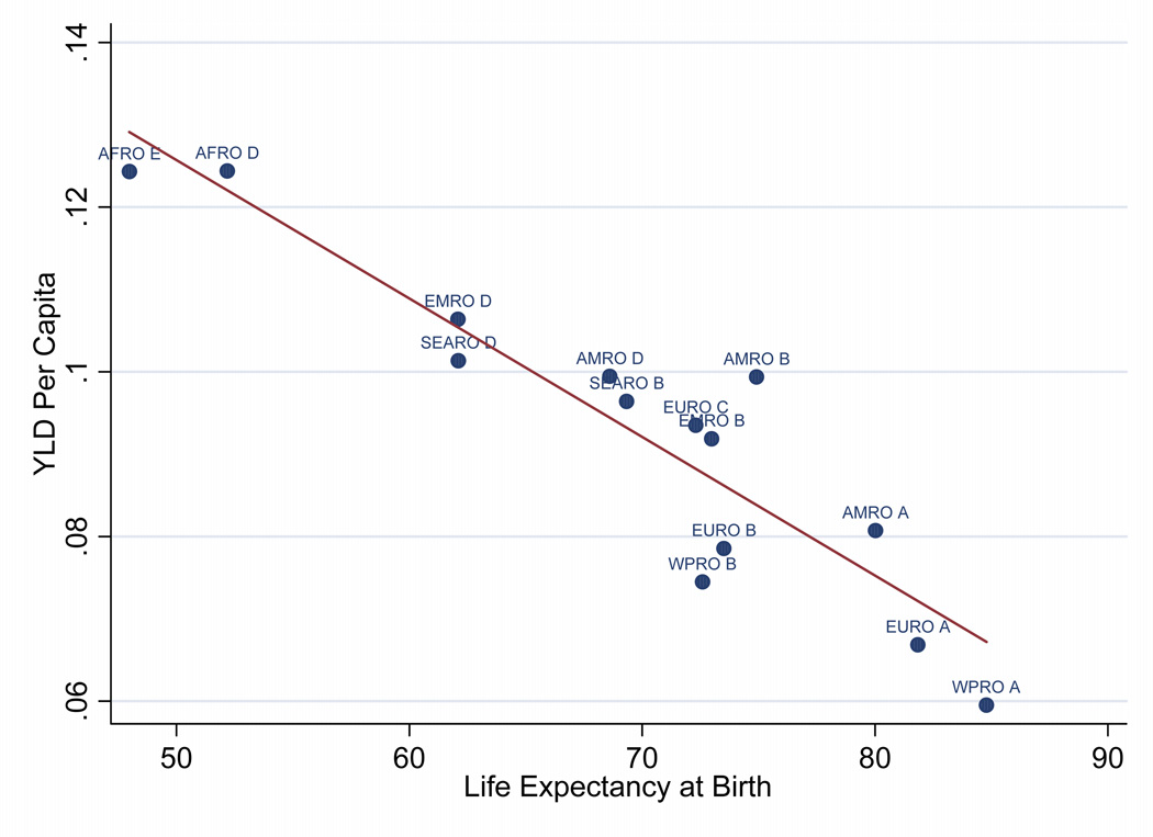
To assess the effect on worker productivity from a general health improvement (i.e., an increase in life expectancy at birth from 40 to 60) we need a mapping from life expectancy to YLDs. We construct this mapping by looking at cross-sectional data from 14 WHO sub-regions on YLDs per capita and life expectancy at birth. Figure 4 shows the data for the full population. In practice, we work with similar data at the age-group level (each group spans approximately 15 years for most of the working-age population). For each age group, we run a regression across the 14 sub-regions of YLDs per capita on life expectancy at birth. The coefficients from these regressions then tell us the change in age-specific YLDs that would result from an increase in life expectancy from 40 to 60. To give a concrete example, the regression of YLDs per capita on life expectancy at birth for the 30–44 age group (with standard errors in parentheses) is:

$$\begin{array}{cccc}YLD=\hfill & 0.251\hfill & -\hfill & 0.00226e_0,R^2=0.88\hfill \\ \hfill & (0.017)\hfill & \hfill & (0.0002)\hfill \end{array}$$

Figure 4.

YLD per Capita and Life Expectancy at Birth

Applying these regression coefficients, a change in life expectancy at birth from 40 to 60 would lower YLDs from 0.160 to 0.115. Using YLDs to measure the impact of disease on labor input is complicated, however, by the fact that diseases at one age may result in disability at another. For example, a crippling disease suffered in childhood will cause disability in adulthood. To take account of this we make the (admittedly extreme) assumption that all YLDs incurred in childhood result in adult disability. Specifically, we spread the YLDs incurred at ages 0–14 evenly over adults aged 15–64. Using the regressions just described, annual YLDs for ages 0–4 fall from 0.221 to 0.148 and annual YLDs for ages 5–14 fall from 0.075 to 0.055. Thus implied YLDs at each adult age due to childhood illness fall from 0.037 to 0.026. The implied labor input per adult in the 30–44 age group after the health improvement relative to before the improvement is thus (1 – 0.115 – 0.026)/(1 – 0.160 – 0.037), or a 7.0 percent increase. Similarly, the implied increases in labor input per worker in the 15–29 and 45–59 age groups are 6.1 percent and 6.6 percent, respectively. These effects are slightly less than half the size of the effects we estimate using the data on ASR. In the simulations below, we use the ASR estimates as the base case.

2.3.2 Phase-in of Health Effects

Conceptually, both the ASR and YLD estimates are derived from thinking about a comparison of workers who have spent their entire lives in a low or high life expectancy environment. However, in response to a health intervention, there will be a long transition period in which some of the labor force will have grown up in a poor health environment. This is important, because there is good evidence that many of the most important health interventions in terms of worker productivity are those that affect young children (or even in utero). Specifically, children who grow up in a more favorable health environment are healthier in a number of measurable respects (such as height, IQ and prevalence of chronic disease), and perform better as students and workers.

To deal with this problem of phase-in, we allow a worker’s health human capital to be a function of both the current health environment and the health environment that prevailed when he was born. In the case of the ASR measure, for example, human capital from health per worker of age i in period t following a health improvement at time T is computed as:

$$h_{i,t}^h=\{\begin{array}{ll}\text{exp}[(1-\eta )\rho ASR+\eta \rho ASR\prime ]\hfill & \text{if}T>t-i\hfill \\ \text{exp}[\rho ASR\prime ]\hfill & \text{if}t-i\ge T\hfill \end{array}$$

where ASR and ASR' are the adult survival rates implied by the mortality regimes prevailing before and after the shock, ρ is the parameter that measures the effect of ASR on worker productivity as estimated by Weil (2007), and η ∈ [0,1] captures the importance of the contemporaneous health environment in affecting worker productivity. A value of η = 1 implies that health improvements are fully reflected in worker productivity right away. A value of η = 0 implies that there is no contemporaneous effect of health improvement on worker productivity; the only workers who will be more productive are those who are born after the improvement in health. At this point we have no solid grounds for estimating the value of η, and so in our simulations we use 0.5 as our base case value.

2.3.3 The Effect of Health on Education

There are several possible channels through which changes in health may increase education. Longer life expectancy increases the time over which investment in human capital can be amortized, and therefore should raise investment in schooling (Kalemli-Ozcan et al., 2000). Lower adult mortality also reduces the number of orphans, who receive less schooling than children with living parents (Case et al., 2004). There is some evidence that healthier children are also better able to take advantage of schooling, for example through reduced absenteeism and greater mental alertness while at school (Bleakley, 2007a). Children may also be kept out of school to provide care for family members who are ill. Another channel is the so-called “quality-quantity” trade-off. If disease eradication and the resulting decline in fertility result in households having fewer surviving children, the household budget constraint – and, at the macro level, the government’s budget constraint – may be loosened, allowing greater investment in each child (Kalemli-Ozcan, 2002).

We calibrate the effect of health on schooling using estimates from Fortson (2007). Fortson examines how the rise of HIV prevalence has affected schooling in a set of seven sub-Saharan countries. She estimates that an increase in adult HIV prevalence from zero to ten percent reduces completed schooling by 0.5 years. Fortson also constructs a theoretical model of optimal schooling’s response to adult mortality, which produces an effect roughly two-thirds as large as the one she estimates.

To translate Fortson’s estimate into a form that we can use, we need to link HIV prevalence and the mortality rate. Based on data on changes in adult mortality and HIV prevalence in her sample, Fortson estimates that ∂mortality/∂HIV is between 0.06 and 0.09. We use the average of these two figures, implying that HIV prevalence of ten percent would raise adult mortality by 0.0075. We can similarly translate the health shock that we are looking at into a change in the adult mortality rate. Using our model life tables, we calculate adult mortality as the average of age-specific mortality for all ages between 15 and 65, weighted by the age-specific population of Sri Lanka in 1953. Adult mortality falls from 0.00972 to 0.00393 when life expectancy at birth rises from 40 to 60. Therefore, the implied change in schooling is:

$$(0.00972-0.00393)\frac{0.5}{0.0075}=0.386$$

In our simulations we thus increase schooling by 0.386 years for all cohorts born after life expectancy rises from 40 to 60. The effect of this rise in schooling on the average level of human capital will depend on the initial level of schooling because, as discussed above, the percentage return to schooling falls with the number of years of schooling. In our base case simulation, we consider the case where initial schooling is below four years, so that the return to schooling is 13.4 percent per year.

2.4 Other Channels from Health to Income

There are several other potential channels from health to income that we do not pursue at this stage.

Changes in health, particularly through changes in adult life expectancy, may also cause changes in the savings rate. Modigliani’s classic life-cycle model of savings would suggest that an increased probability of surviving past the age of effective labor force participation would increase savings rates in the long run. In the short run, the demographic bulge of relatively young workers saving at a relatively high rate might also increase capital accumulation relatively shortly after the shock. Although these mechanisms may be important, it remains difficult to judge quantitatively how important life-cycle savings effects are likely to be in a developing economy. There is a lively discussion of the evidence on these issues as they relate to Taiwan in Lee et al. (2001) and Deaton (1999).

Reduced fertility that accompanies lower mortality will also have a positive effect on labor supply, particularly for women. This effect has been explored recently by Bloom et al. (2007) for the case of fertility declines resulting from changes in abortion laws. In the experiment we consider, of raising life expectancy at birth from 40 to 60, the total fertility rate falls from 5.16 to 3.72. Thus, the average woman has 1.44 fewer children in the healthy regime. However, because much of the difference in life expectancy results from mortality at young ages, the difference in time required for child care is much smaller than the difference in the number of children ever born.

3 Basic Results and Sensitivity

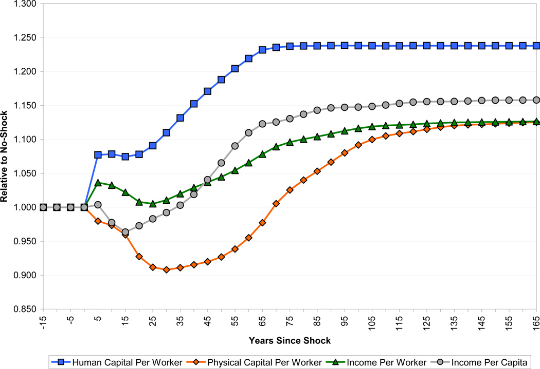
Figure 5 shows the results of our simulation for a “base case” set of parameters. These are a fertility adjustment period of 50 years, health impact on productivity calculated according to the ASR methodology, a phase-in effect of health on the productivity of those born before the improvement (the parameter η) of one-half, initial schooling of less than four years, an economy closed to international capital flows, and a land share in the Cobb-Douglas production function of 10 percent. Figure 5 shows the levels of human capital per worker, physical capital per worker, output per worker, and output per capita. As in all the figures that follow, we show results relative to a baseline in which no health improvement takes place.

Figure 5.

The Base Case Scenario

The evolution of human capital per worker shows a combination of the direct effect of the health shock on labor productivity, the increase in schooling due to better health, and the changing age-structure, and therefore experience, of the workforce. The long-run effect of the changed age-structure of the workforce is to increase per worker human capital by about 2.1 percent, and that from schooling is 6.2 percent. The long-run effect of higher productivity due to health is 15.5 percent. As is clear from the figure, much of the benefit of better health for human capital – specifically, all of the schooling effect, half of the direct health effect, and all of the experience effect – is subject to a significant time lag.

Physical capital per worker falls following the shock mechanically because more workers are now alive to work with the same aggregate amount of capital. Since much of the increase in life expectancy is among the young, the cohorts entering the labor force after the shock are substantially larger than earlier incoming cohorts. This has the effect of depressing the capital stock per worker still further. Eventually, as the size of the population stabilizes, increased savings from the extra workers lead to a gradual recovery in the capital-labor ratio. The capital-labor ratio reaches a minimum about thirty years after the shock, at which point it is about 10 percent lower than it was before the shock.

The path of output per worker reflects the dynamics of human and physical capital per worker, as well as land per worker (which we do not show, but which can be inferred from Figure 5). Output per worker follows an odd path, initially rising from the improvement in worker productivity due to better health, then falling due to capital and land dilution from faster population growth, and eventually rising again as population growth slows and the benefits of better health through schooling and the productivity of later-born cohorts phase in. As discussed above, the demographic dynamics of our model determine the gap between income per worker and income per capita. For the first 40 or so years after the health improvement, a higher dependency ratio means that income per capita is lower relative to baseline than is income per worker. In the steady state, income per capita is 3.2 percent higher relative to baseline than income per worker.

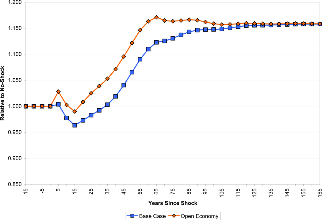
Figure 5 shows that in our base case the long-run effect of better health is to raise output per capita by roughly 15 percent relative to the baseline of no health improvement. In the sense that better health raises income, this result is a confirmation of the widely accepted view that health provides economic benefits. However, both the magnitude and timing of the effect are disappointing from this perspective. An increase in life expectancy from 40 to 60 is a major health improvement, and our simulation says that such an improvement would have a very small effect on the income gap between the typical rich and poor countries. Further, for the first thirty years following a health improvement, income per capita is lower than it would have been had health not improved.

We now turn to an examination of the sensitivity of these basic results to some of the modeling choices and parameters that we have used.

3.1 The Effect of Health on Productivity

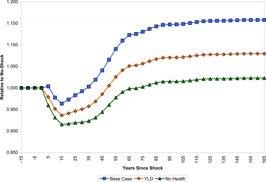
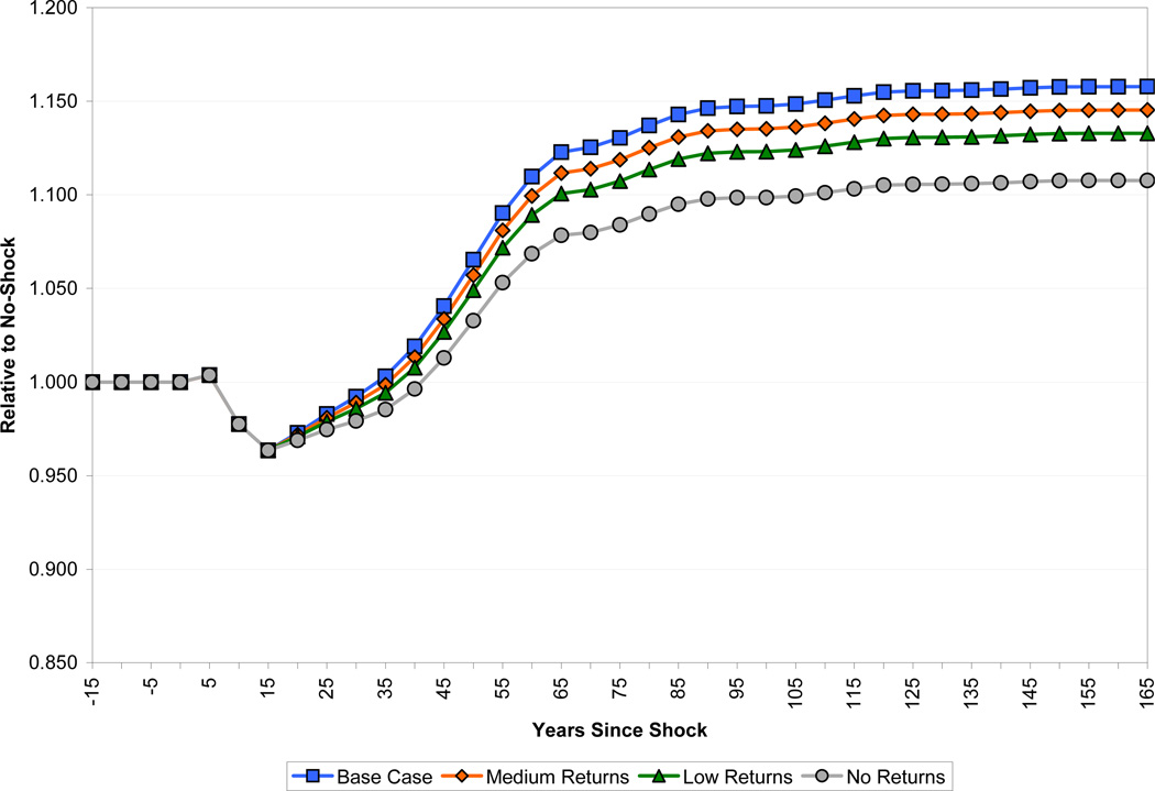
As discussed above, our base case analysis uses an estimate of the effect of health on labor productivity (the ASR measure) based on estimates in Weil (2007). We also have an alternative measure of these productivity effects built up from information on years of life lost to disability (the YLD measure). Figure 6 shows the paths of output per capita following a health improvement for these two cases, and also for the case in which we assume a zero effect of health on worker productivity. In all cases, the paths of population, schooling, and labor force experience are the same. The YLD results paint a more negative picture than the ASR results, because the positive effect on health human capital is only about half as large. After 15 years, income falls by more than one and a half times as in the ASR case, and recovery is much more protracted, taking about 50 years rather than 35 years. The long-run positive effect is about half as large as the ASR measure.

Figure 6.

Effect of Health on Income per Capita

The fact that income per capita scarcely rises at all in the long run for the “No Health” case indicates that the favorable effects of health on schooling, experience, and the dependency ratio alone roughly equal in magnitude to the negative effect of increased population, working through greater pressure on the fixed factor.

3.2 The Phase-in of Health Improvements

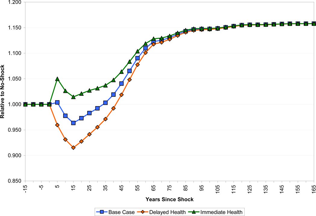
In our base case, we assumed a value for η, the parameter that describes the phase-in of productivity benefits from health improvements, of one-half. This means that people already alive at the time of an improvement in health receive half of the benefit that accrues to those who are born after. Figure 7 shows the path of income per capita in this base case along with paths for the cases of η = 0 and η = 1. By construction, the steady states of these three scenarios are the same, since eventually all of the people alive at the time of the health improvement have died.

Figure 7.

The Phase-in Effect on Income per Capita

In the case in which returns to health accrue only to those not yet born, the negative effect of health on income is little more than double the baseline case, with a fall of about 8.5 percent after 15 years. However, the dynamics are little affected, with income per capita recovering to baseline only 5 years later than in the base case scenario.

In contrast, the dynamics are markedly different if those currently alive receive all of the benefits of a health shock. The positive effects on human capital are large enough to entirely offset the capital shallowing that results from the larger population, with income in all years after the shock greater than in the no-shock case, although by a very small margin for the period from 10–30 years after the shock when the capital-shallowing and dependency effects are at their greatest.

3.3 The Returns to Schooling and Experience

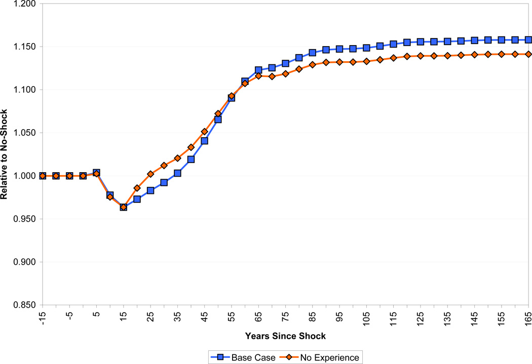
Figures 8 and 9 highlight the role of experience and the return to schooling in the model. We show the path of output in the base case, and then the results of setting the return to experience to zero (holding fixed the return to schooling) in Figure 8, and setting the return to schooling to different possible levels (holding fixed the return to experience) in Figure 9. Accounting for the human capital acquired through experience somewhat increases the amplitude of the changes following the shock. When the experience effect is deleted, output is higher than the base case during the period from 15 to 50 years after the change in health, because during this time the average age of the labor force is below its base-case level. After that, however, the long-run shift in the age-structure of the population is towards slightly older workers. In the steady state, income per capita is higher (by about 1.7 percent) in the case where experience is accounted for than in the case where it is ignored.

Figure 8.

Effect of Worker Experience on Income per Capita

Figure 9.

Effect of Schooling on Income per Capita

In the case of education, our base case assumption was that the return to additional education was 13.4 percent per year, which is consistent with initial education being below four years. Indeed, this may have been reasonable for some countries at the time of the international epidemiological transition, but looking forward, there are few countries in the world with education this low today. We show alternative paths for the simulation using lower returns to education (i.e., 10.1 and 6.8 percent), and for the case where the return to education is zero.

The key point concerning all of these results is that, although the long-run effects of the shock on the economy naturally differ, the dynamic effects of the shock are almost identical regardless of the assumed returns to education. The income loss at 15 years is exactly the same (since none of the new workers affected by schooling have yet entered the labor force), and regaining the no-shock income level occurs only 5 years later if there are no returns to schooling at all than if there are the relatively high returns assumed in our baseline case.

3.4 The Speed of Adjustment of Fertility

Acemoglu and Johnson (2007) explain their finding that health improvements did not result in economic growth during the international epidemiological transition by arguing that population growth undid any direct positive effects of health. In our model, these population effects run through crowding of land, temporary reductions in capital per worker, and a temporary rise of the dependency ratio.

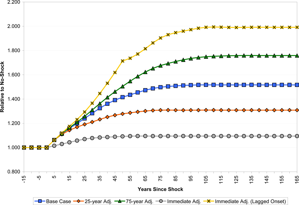
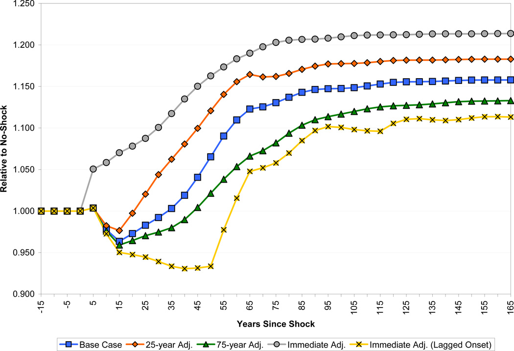
Figures 10 and 11 show how the results are changed by changing the horizon over which fertility adjusts. The base case assumed that it would take 50 years for fertility to adjust to its new long-run rate. Fifty years seems broadly plausible, since conventional wisdom suggests that demographic transition typically takes place over the course of about two generations. However, estimates of the response of fertility to mortality changes, and the lag with which they occur are remarkably imprecise, and, moreover, subject to considerable regional variation. It is commonly accepted, for example, that the African transition has been unusually prolonged. Transition in Latin America and Asia, despite their massively different social and economic circumstances, took a similar amount of time, with widespread falls in fertility fairly apparent by the 1980s (Cleland, 2001). Therefore, the figures also show fertility adjustments that take 25 years, which is perhaps a little closer to the historical experience of fertility adjustment in East Asia, or 75 years, which is perhaps closer to the historical experience of Europe or the experience of some sub-Saharan African countries in the more recent past (Lee et al., 2001). We also show the paths for the case in which fertility adjusts instantaneously to the change in mortality and the case in which fertility does not adjust at all for 50 years following with shock, then adjusts in one jump to the level consistent with the pre-shock level of population growth.

Figure 10.

Effect of Adjustment Speed on Population Size

Figure 11.

Effect of Adjustment Speed on Income per Capita

Figure 10 shows the path of population size under the different scenarios. Relative to baseline in which there is no change in life expectancy, the long-run increases in population are 31 percent, 52 percent and 76 percent respectively as fertility takes 25, 50 and 75 years to adjust. Differences in the rate of fertility adjustment become apparent only fairly gradually. After 25 years, the population is 20 percent, 24 percent and 26 percent bigger in the three scenarios. After 50 years, however, the differences are apparent, with population increase being only 27 percent in the 25-year adjustment case, but 42 percent in the base case and over 50 percent in the 75-year adjustment case. When fertility adjusts immediately to the change in mortality, there is still a slight increase in population size relative to the baseline, reflecting higher survival beyond childbearing years.

Figure 11 shows the corresponding paths for income per capita. Not surprisingly, slower adjustment of fertility exaggerates the short-run fall in income per capita and reduces the long-run increase. In the gradual-adjustment scenarios, the fall in income per capita 15 years after the shock is between 2.5 and 4 percent. Income per capita recovers to the baseline level after about 20, 35 and 45 years after the shock respectively. The long-run economic benefits of improved health are also reduced when fertility is slower to adjust. The 25-year adjustment case leads to long-run income gains of about 18 percent, while the 75-year adjustment case raises income by only about 13 percent. These long-run effects run entirely through the land-labor ratio.

The population dynamics in our model are entirely generated by our assumptions about fertility adjustment. An interesting exercise is to see how they compare to the population dynamics underlying Acemoglu and Johnson’s (2007) findings. As a first step we can look at their estimate of the effect of health improvements on population size. Specifically, we look at the coefficient from a regression of change in log population size from 1940 to 1980 on the change in log life expectancy over the same period, where the change in life expectancy is instrumented using predicted mortality. The coefficient is 1.67 with a standard error of 0.50 (Table 8, column 1). The coefficient implies that an increase in life expectancy from 40 to 60 would raise population size by a factor of 1.97 over this 40-year period (using a coefficient two standard errors below their estimate implies an increase in population size by 31 percent after forty years). By contrast, in our base case simulation, the effect on population after 40 years is a 36 percent increase, and even allowing for a 75-year adjustment for fertility the increase after 40 years is only 41 percent. Further, the simulation we run is not fully comparable to the experience on which Acemoglu and Johnson base their analysis, since we assume that the entire improvement in life expectancy takes place instantly, whereas in reality the change was phased in (although heavily weighted toward the beginning of the period.) Since Acemoglu and Johnson also report estimates of the share of the population under 20, we can use this as an additional check on our experiment. Their coefficient is 0.12, implying the share of the population under 20 is 4.9 percentage points higher than otherwise under our shock. At a forty year horizon, in our base case the share of the population under 20 peaks at 2.5 percentage points above the pre-shock level after 15 years, but by 40 years has almost exactly reached its pre-shock level.

What explains the failure of our simulated population to line up with Acemoglu and Johnson’s estimates? One possibility is that the health improvement being studied (for which life expectancy is a proxy) affected population not only through reduced mortality, but also through higher fertility. Higher fertility in this story would have to be the direct result of better health (it couldn’t be the result of higher income, since Acemoglu and Johnson find that better health did not raise income). Such a story has some support. For example, Lucas (2007a) finds that malaria eradication in Sri Lanka raised fertility, which is consistent with evidence that malaria reduced fecundity.

Another possibility is that there is something wrong with the Acemoglu and Johnson instrument for changes in life expectancy. If instrumented increases in life expectancy produce more population growth than can be accounted for by the decline in mortality, it may be that the instrument is correlated with the part of fertility not related to mortality. In other words, countries with high mortality reductions might also just have high levels of fertility (or slow declines in fertility). We do not have a particular theory that produces this correlation, but obviously if it is present it also calls into question the other results that Acemoglu and Johnson derive regarding the effect of life expectancy on income.

To see whether our results would match the Acemoglu and Johnson results if our population path had matched theirs, we conducted the following experiment: we used our demographic model to ask how much fertility would have to jump up at the time of the mortality decline (assuming that fertility then remained flat) in order to match the Acemoglu-Johnson finding that (for the mortality decline we consider) population will be 1.97 times the baseline level after 40 years. The answer is that fertility would have to rise by a factor of 1.24. We then fed this demographic scenario through our economic model. The result is that output per capita at a 40 year horizon would be 20 percent below baseline (recall that in our base case scenario, output per capita at a horizon of 40 years is 2 percent above baseline). By contrast, Acemoglu and Johnson’s coefficient from an instrumented regression of log GDP per capita on log life expectancy is −1.32 (Table 9, column 1), implying that the mortality improvement we consider would lower GDP per capita by 41 percent. This finding suggests that differences between our findings and those of Acemoglu and Johnson are due to differences in both demographics and non-demographic factors, in roughly equal proportions.

This is a convenient point at which to discuss the relationship between our paper and those by Alwyn Young. Young (2005) simulates the effect of the AIDS epidemic in South Africa on per capita income, using a Solow model, along with his own econometric estimates of changes in the participation rate and fertility, and an assumption that orphans accumulate no further human capital after they are orphaned. This exercise, and its successor concerning sub-Saharan Africa (Young, 2007), is similar in spirit to the present work, although, since it concerns a particular disease, it can naturally be more precise about certain behavioral responses. Relative to our work, however, Young is more concerned with long-run effects whereas we emphasize transition paths. Our methodological approach is also somewhat different from that of Young, in that we rely as heavily as possible on well-identified econometric estimates produced by other authors, rather than on producing our own estimates.

Although the approach in Young’s papers is broadly similar to that in ours, and although we share his assumption that reductions in health reduce human capital accumulation, we differ from him crucially in our assumptions concerning fertility. Young’s work is important and surprising because it argues that a massive increase in mortality actually reduces fertility; precisely the opposite of the normal assumption, that increases in mortality increase fertility. Young’s views on the effect of HIV/AIDS on fertility are not uncontroversial, and Kalemli-Ozcan (2008) makes precisely the contrary argument, that the epidemic has caused an increase in fertility. There may be a number of mechanisms at work, including a decline in the demand for unprotected sexual activity, emphasized in Young (2005), and an independent decline in demand for children (Young, 2007). None of the mechanisms in question, however, are likely to shed light on the response of fertility to changes in the general infectious disease environment or to malaria or tuberculosis in particular. For example, HIV/AIDS may reduce demand for children among infected parents concerned that their children are likely to be orphaned young. This is unlikely to be a factor in the case of malaria, which has relatively little effect on adults in infected areas. Similarly, the long interval between HIV infection and the development of AIDS presumably leaves more time for changes in fertility behavior than the relatively quick onset of adult tuberculosis.

3.5 The Role of Land in the Production Function

Our base case treatment of land involved assuming both a particular functional form (Cobb-Douglas, in other words unit elasticity of substitution) and a particular exponent on land in the production function. In this section we relax both of these assumptions. We adopt a CES production function in which we can specify an elasticity of substitution between a capital-labor-technology composite factor, on the one hand, and the fixed factor on the other:

$$Y_t={[(1-a){\left(A_t{K}_t^{\alpha }{H}_t^{1-\alpha }\right)}^{\frac{\sigma -1}{\sigma }}+a{X}^{\frac{\sigma -1}{\sigma }}]}^{\frac{\sigma }{\sigma -1}}$$

where σ is the elasticity of substitution. If the fixed factor is paid its marginal product then its share of national income at time t, ϕ_t, will be:

$${\varphi }_t=\frac{a{X}^{\frac{\sigma -1}{\sigma }}}{(1-a){\left(A_t{K}_t^{\alpha }{H}_t^{1-\alpha }\right)}^{\frac{\sigma -1}{\sigma }}+a{X}^{\frac{\sigma -1}{\sigma }}}$$

If the elasticity of substitution is not unity, the fixed factor’s share of national income will vary as capital and human capital are accumulated, population grows, and technology improves. For example if σ > 1, so that other factors can substitute for the fixed factor, then the fixed factor’s share of income will decline over time. Thus, one should be able to learn about the elasticity of substitution, at least in a gross sense, by observing how the income share of the fixed factor changes over time, as A, K, and H accumulate.

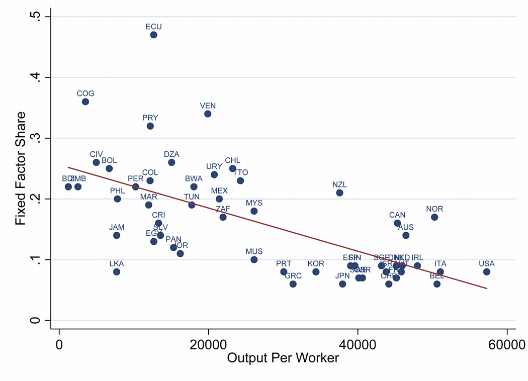
Figure 12 shows data for doing such an analysis. The horizontal axis measures output per worker. The data on the vertical axis is an estimate of the income share of non-reproducible factors of production, from Caselli and Feyrer (2007).⁶ The Caselli and Feyrer estimates are in turn built on data from World Bank (2005) on the values of physical capital, crop land, pasture land, and subsoil resources. In the cross section, there is a clear negative relationship between the level of output and the share of the fixed factor. Combining the production function and the expression for the income share of the fixed factor, putting everything in per worker terms, and re-arranging, we get:

$$\text{ln}({\varphi }_i)=\text{ln}(a)-\frac{\sigma -1}{\sigma }\text{ln}(y_i/x_i)$$

where xi is fixed resources per worker and y_i is output per worker, and we are now considering a cross-section of countries. The results (with standard errors in parentheses) from running this regression are:

$$\begin{array}{cccc}\text{ln}({\varphi }_i)=\hfill & -2.233\hfill & -\hfill & 0.574\text{ln}(y_i/x_i),R^2=0.56\hfill \\ \hfill & (0.069)\hfill & \hfill & (0.071)\hfill \end{array}$$

The implied value of σ, the elasticity of substitution, is 2.35 with a 95 percent confidence interval of [1.56, 3.13]. We know of few estimates of this parameter to compare to our own. Nordhaus and Tobin (1972, Appendix B), using time series data for the US over the period 1909–1958 on capital and labor stocks and the income share of natural resources, estimate the elasticity of substitution between land and a labor-capital aggregate as 2.02.

Figure 12.

Fixed Factor Income Share and Output per Worker

Figure 12 is also informative about the share of fixed factors in national income. Our base case, in which the land share is 10 percent, is probably quite conservative for most developing countries. Other evidence also suggests this. In a well-known study, Hansen and Prescott (2002) assume a value of 30 percent for pre-industrial economies. Accordingly, a sensitivity analysis that increases land’s share of national income to 20 or even 30 percent seems reasonable for at least some developing countries.

The production function can be re-written to show how total output compares at two points in time, as the quantities of physical and human capital along with the level of productivity change.

$$\frac{Y_s}{Y_t}={[(1-{\varphi }_t){\left(\frac{A_s{K}_s^{\alpha }{H}_s^{1-\alpha }}{A_s{K}_s^{\alpha }{H}_s^{1-\alpha }}\right)}^{\frac{\sigma -1}{\sigma }}+{\varphi }_t]}^{\frac{\sigma }{\sigma -1}}$$

To do this comparison one does not need to know the quantity of the fixed factor X or the parameter a, but only the income share of the fixed factor at a point in time, the elasticity of substitution, and the growth of the inputs into production, all of which we were already measuring. We use a value of $\alpha =\frac{1}{3}$, which is consistent with our earlier parameterization of giving capital a 0.3 exponent when the land share is 10 percent.

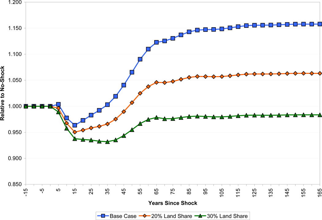
Figure 13 shows how the results of the model are altered when the income share of land is increased from 10 percent to 20 and 30 percent. There are significant differences between the three simulations in GDP per capita following the shock. In comparison to the base case, it takes income an additional 15 years to recover to its pre-shock level under a 20 percent income share of land. A recovery never occurs when land’s share is 30 percent. The simulations also have markedly different implications for the long-run gains from improvements in health. For instance, doubling the share of land more than halves the long-run gains in per capita income from improved health, which go from about 16 percent to 6 percent. Naturally, the longer fertility takes to adjust, the more pronounced this effect will be.

Figure 13.

Effect of Land Share on Income per Capita

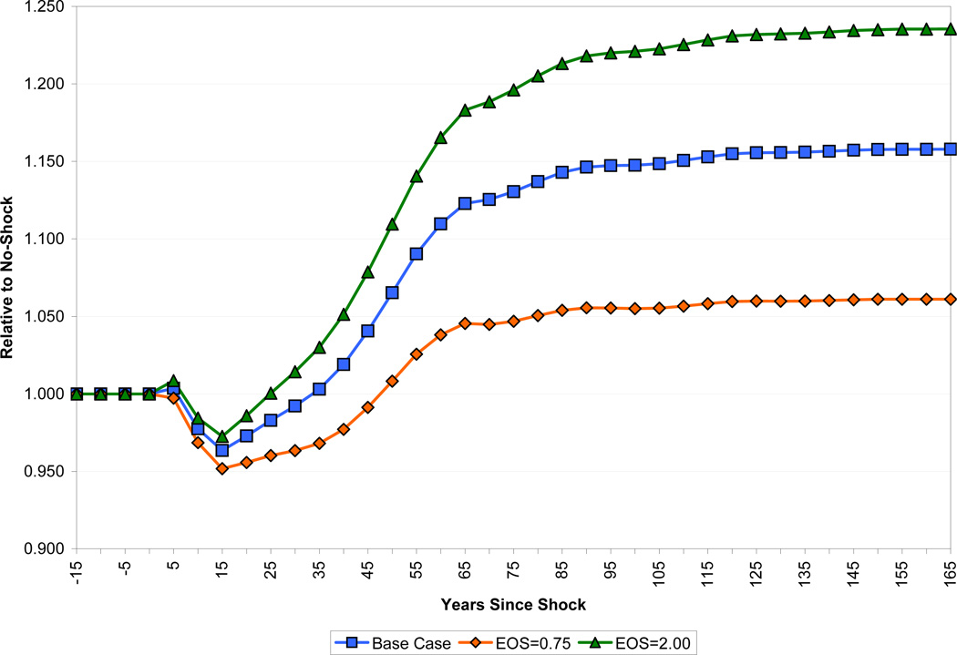
We now turn to the elasticity of substitution between the fixed factor and other inputs to production. Intuitively, the greater this substitutability, the less severe will be the consequences of increased population pressure on the fixed factor following the shock. Figure 14 shows how varying the elasticity parameter σ influences our findings by comparing our base case scenario with results obtained under σ = 0.75, where land is more complementary than in the Cobb-Douglas case, and under σ = 2, where land is more substitutable. While it takes income per capita about 50 years following the shock to recover to its pre-shock level under σ = 0.75, this recovery occurs in 25 years when land is twice as substitutable as in the Cobb-Douglas case. Moreover, the long-run gains in income per capita also increase with greater substitutability of the fixed factor, rising from 16 percent to 24 percent as the elasticity of substitution doubles from unity in the Cobb-Douglas case.

Figure 14.

Effect of Land Substitutability on Income per Capita

Finally, we consider a case that may be relevant for many resource rich developing countries, in which there is a large resource extraction sector that is largely detached from the rest of the economy. Specifically, we set the resource share in national income to 40 percent and the elasticity of substitution between resources and other inputs to infinity. Coincidentally, these two changes almost exactly cancel each other out, so that the path of income looks very similar to our base case. Income per capita has the same initial dip as in the base case, and regains its initial baseline after 30 years, as compared to 35 years in the base case. After 50 years, income per capita is 9.0 percent above baseline, as compared to 6.5 percent in the base case.

3.6 International Capital Flows

An important part of our results is driven by the assumption of Solovian saving. It is possible to adjust this assumption in a straightforward way even without building a life-cycle savings model, simply by assuming that the economy is open to international capital flows that equalize the return to capital around the world, at least up to a country fixed effect.⁷

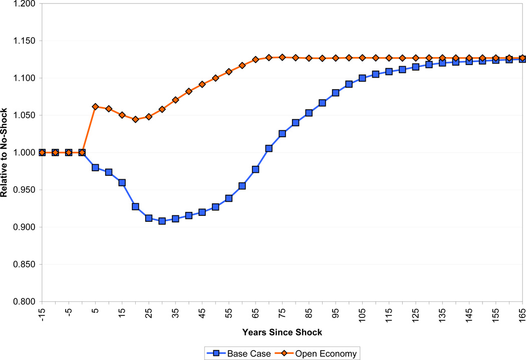
Figures 15 (capital per worker) and 16 (income per capita) show that allowing for capital flows (assuming a fixed world interest rate) does indeed significantly change the results.⁸ In the closed economy case, capital per worker falls monotonically to a minimum of about 90 percent of baseline thirty years after the shock. In the open economy case, capital per worker stays close to the no-shock case over the first couple of decades after the shock. This is because the effects of increased human capital, which draws capital per worker into the economy, are still only phasing in, while there is a significant drag on returns to capital from the presence of the fixed factor. From about twenty-five years after the shock, however, the effects of increased human capital begin to make themselves felt more strongly, and the capital stock quickly converges to its long-run level, about 13 percent higher than in the no-shock baseline. Thirty-five years after health improvement, income per capita is 5 percent above the baseline path in the case of an economy open to capital flows, while it has barely regained the baseline level in the closed economy. Even 65 years after the shock, income per capita is 5 percent higher in the open economy than in the economy reliant on domestic savings.

Figure 15.

Effect of International Capital Flows on Capital per Worker

Figure 16.

Effect of International Capital Flows on Income per Capita

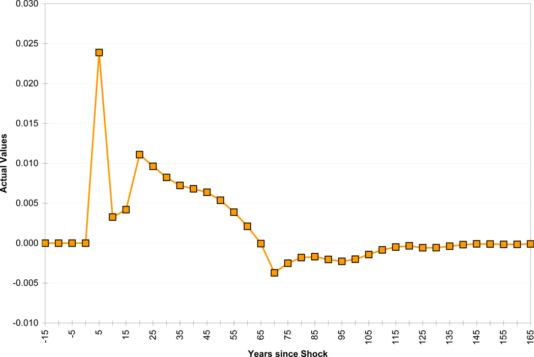
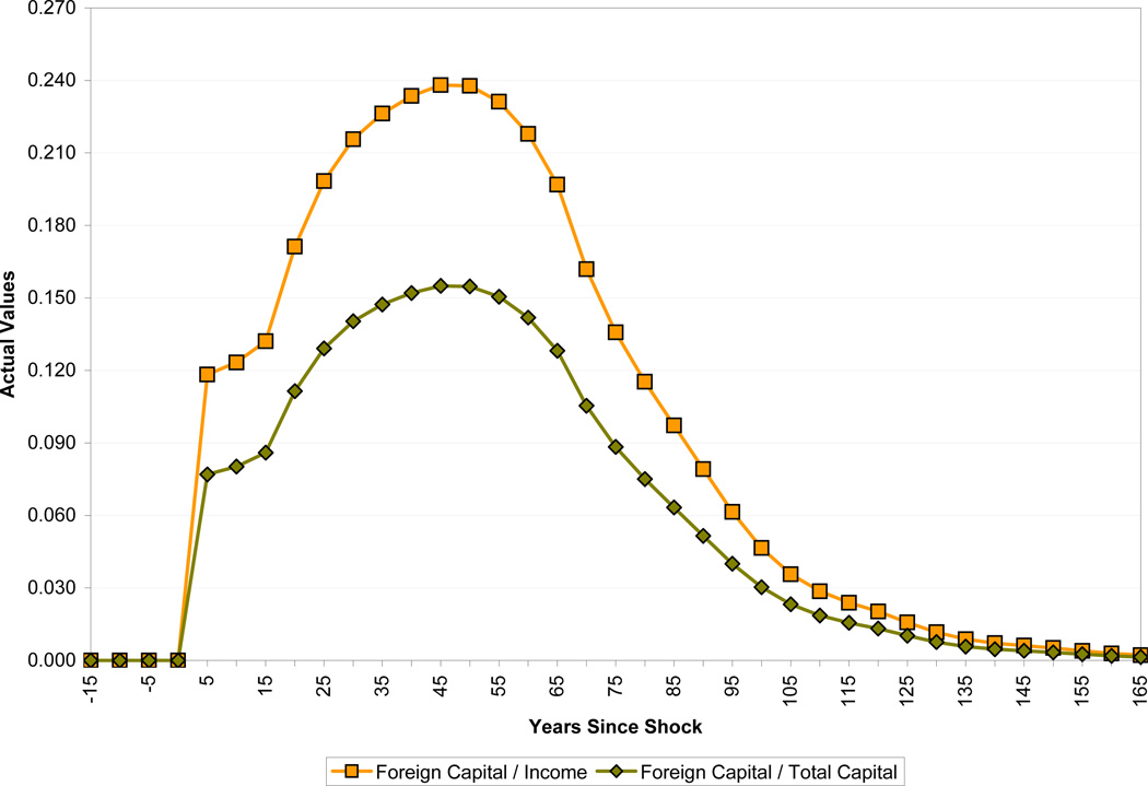
The most important question to ask about this case is whether capital flows of the magnitude envisaged could be sustained by developing economies. Figure 17 shows the resulting current account deficit as a percentage of GDP, and Figure 18 the size of foreign capital required over the period, both as a percentage of GDP and of total capital. The current account deficit resulting from this source of capital inflow spikes at 2.5 percent of GDP in the first five years after the shock, as the productivity of current workers jumps from the improvement in health. The current account deficit then declines for a decade before rising to about one percent of GDP for several decades due to the health-induced rise in population growth. The ratio of foreign debt to GDP peaks about half a century after the shock, at about 25 percent (equivalent to 15 percent of the capital stock). While these numbers are probably manageable in themselves, they are not small increments to the respective measures, so could well be difficult to sustain in countries with substantial accumulated debt, whether public or private. Accordingly, the open economy results highlight the importance of maintaining institutions and policies favorable to foreign investment, including, but not limited to, avoiding substantial government indebtedness.

Figure 17.

The Current Account Deficit as a Percentage of Income

Figure 18.

The Evolution of Foreign Capital

3.7 “Best Case” and “Worst Case” Scenarios

The reader can see from the above exercises how varying individual assumptions of our simulation model affects the results. Obviously it is possible to vary more than one assumption at a time, and the effects of doing this will not likely be simply a sum of the results from varying them individually. There is no problem running such scenarios through our simulator. The difficulty is in summarizing the immense number of potential results. Here we consider two scenarios of interest.

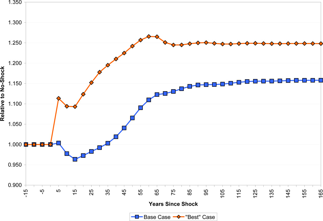
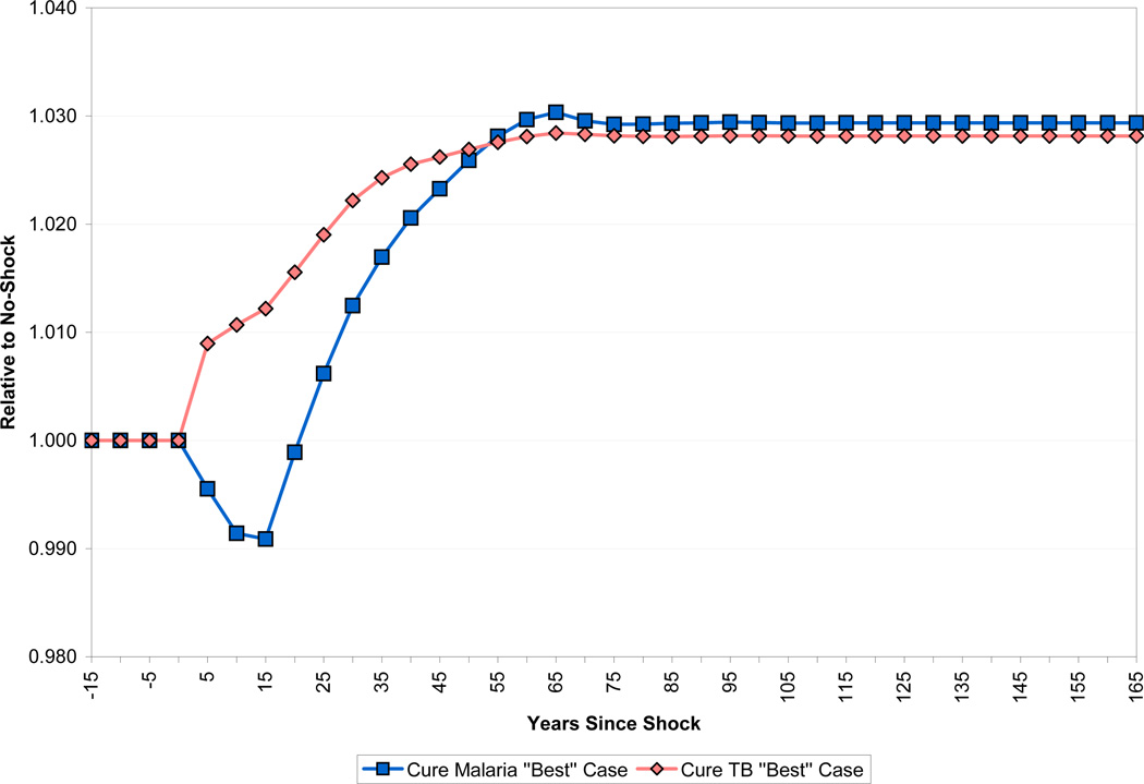
We start by considering a “best case” for the effects of health on growth. That is, we choose parameters that give the largest effect of health on growth while at the same time being reasonable within the framework that we have constructed. Specifically, compared to the base case, we make the following adjustments. We set the speed of fertility adjustment to 25 years, set the elasticity of substitution between land and other inputs to 2 (keeping the land share in national income at 10 percent), and consider the case of an economy open to capital flows from abroad. We leave the treatment of experience and schooling at their base case values (the latter is already arguably optimistic). Finally, for the effect of health on worker productivity, we assume a value of η = 1, implying that improvements in health are reflected in worker productivity right away. In this scenario, income per capita rises immediately by 10 percent in response to the health improvement as shown in Figure 19. After 40 years, income is 21 percent above baseline, and in the steady state income is 25 percent higher than baseline. Compared to the base case, the best case scenario tells a significantly more positive story about the ability of health improvements to raise the standard of living. This being said, however, even in this case the response of income to health is far lower than one would expect from popular pronouncements on the issue.

Figure 19.

The Best Case Scenario for Income per Capita

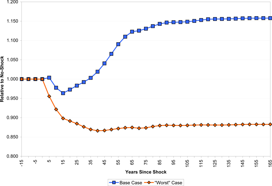
The second scenario we consider is a “worst case,” designed to minimize the effect of health on economic growth, again subject to the constraint of picking parameters that seem to us somewhat reasonable. Specifically, we set the speed of fertility adjustment to 75 years, land’s exponent in the production function to 0.3, the elasticity of substitution between land and other factors to one, and the parameter governing the phase-in of productive effects of health (η) at zero, implying that only those born after the health improvement have increased productivity. We consider the case of an economy closed to international capital flows. Finally, we use the “YLD” method for calculating the productive benefits of better health, rather than the “ASR” method used in our standard simulations. Figure 20 shows the results. With these parameters, our standard improvement in health lowers income per capita not only in the short run (as in the base case scenario) but in the long run as well. At a 40 year horizon, income per capita is 13.4 percent below its baseline path. Although this scenario certainly contradicts the conventional wisdom that health improvements lead to economic growth, it still does not match the findings of Acemoglu and Johnson (2007). Recall that in their analysis, the mortality improvement considered here would lower GDP per capita by 41 percent after 40 years.

Figure 20.

The Worst Case Scenario for Income per Capita

4 Disease Eradication

Thus far in the paper, the health improvement that we have been considering has been an increase in life expectancy at birth from 40 to 60 years, which is meant to roughly match the international epidemiological transition that took place in the decades following World War II. The components of that transition included the widespread availability of antibiotics, new vaccines, the use of DDT, and the creation of public health infrastructure in a large number of countries. The improvement in life expectancy resulted from progress against many different diseases which affected individuals at different ages and had varying effects on labor productivity and human capital accumulation.

We now turn to examine the effects of more specific health improvements. That is, we look at the effects of eradicating specific diseases. We also adopt a prospective, rather than historical approach. In other words, we start from the current health conditions and ask how things would change if the disease environment were altered. The pairing of the disease-specific and prospective approaches (and similarly the general health and historical approaches) is not a logical necessity. We could use our model to ask about general health improvements starting from the current situation, or similarly about what the effect was of progress against specific diseases in the past. We adopt the approach we do out of considerations of data availability and policy relevance.

The two diseases we consider are malaria and tuberculosis. Both are major killers in developing countries, and both are at the center of recent international efforts. (The third disease that naturally falls into this category is HIV/AIDS. However, this disease presents a number of complications that make it too difficult for us to deal with for now.) In both cases, we consider the effect of immediately eradicating the disease in question. Disease reductions that fell short of complete eradication, or which were phased in gradually, would obviously have effects that were smaller than those shown here.

We apply our model to demographic data from Zambia, which is fairly representative of sub-Saharan Africa as a whole. In 2001, its life expectancy at birth was 37 years. Malaria was the cause of about 8.3 percent of deaths in Zambia, compared with a sub-Saharan average of 9.8 percent. Tuberculosis was a little more severe than the sub-Saharan average, causing about 3.1 percent of deaths compared with 2.0 percent on average.

Eradicating tuberculosis raises life expectancy at birth from 37.0 years to 38.0 years. Eliminating malaria would raise life expectancy at birth to 38.6 years. These gains in life expectancy at birth are very small compared to the 20 years that characterized the international demographic transition in the previous experiment. Their economic effects will naturally also be substantially smaller.

Applying our simulation model to specific diseases requires several modifications. When we considered general improvements in health, we used data on mortality (that is, life expectancy at birth) as an indicator of morbidity, that is, how healthy the surviving population was. Individual diseases, however, will not have the same relative effects on morbidity and mortality as the general health improvement that we considered above. For example, among adults, malaria has a large effect on morbidity relative to mortality. Thus when we consider individual diseases, we de-couple morbidity and mortality. We use direct measures of the morbidity effects of individual diseases as well as their age-specific mortality profiles. We also alter our treatment of the effect of disease prevalence on school completion (in the case of malaria, but not tuberculosis), to take advantage of good estimates of this particular effect.

The pieces of our model other than demographics, productivity effects of disease, and schooling effects of disease are the same as those discussed above.

4.1 Demographic Effects of Disease Eradication

The pre-shock mortality regime is generated from life table data for Zambia in 2001, obtained from the WHO. To simulate the appropriate shocks, we use data from the WHO on disease-specific deaths to create the corresponding cause-deleted life tables, which are then applied in the respective scenarios to project the population from the shock period (i.e., year 0) onward.⁹ For pre-shock fertility, we use age-specific fertility rates reported for Zambia in 2001 by the US Census Bureau’s International Data Base.

Figure 21 shows the level of the population following the eradication of the diseases. Since malaria accounts for a greater fraction of mortality than tuberculosis, and this mortality is concentrated at younger ages, not surprisingly the increase in population resulting from its eradication is also larger: about 5 percent in the long run compared with about 2.7 percent in the long run for tuberculosis. In both cases, around 80 percent of the extra population growth occurs in the first forty years after the shock.

Figure 21.

Effect of Disease Eradication on Population Size

Figure 22 shows the most substantial economic difference in the effect of eliminating the two diseases. Eliminating malaria causes the dependency ratio to increase by about 2.6 percent over the following 15 years, while eliminating tuberculosis causes the dependency ratio to fall more or less continuously for the next 60 years, including on impact. It is worth noting that the dependency ratio implied by the Zambian life tables is significantly higher before the shock than that implied by the South Asian model life tables in the earlier experiment. Before the shock, the dependency ratio is about 0.95 using these life tables, compared with only about 0.69 in the previous experiment.

Figure 22.

Effect of Disease Eradication on the Dependency Ratio

4.2 The Direct Effect of Disease on Labor Productivity

To measure the effects of eradicating specific diseases on labor productivity, we use data on age-specific disease prevalence from the Global Burden of Disease (GBD) project (Murray and Lopez, 1996). The data apply to sub-Saharan Africa. In the case of malaria, we look at both episodes of the disease and the neurological sequelae that result from cerebral malaria in children under five. Prevalence is defined as the fraction of a year that the average person in an age group experiences a disease. In the case of malaria episodes, for example, 17.5 percent of adults experience an episode every year, but duration is quite short, so the prevalence of the disease is only one-quarter of one percent. By contrast neurological sequelae have no incidence among adults, but a prevalence of more than half a percent because they last a lifetime.

In principle, the data on prevalence should be combined with a disability weight to produce a measure of how much of the adult population’s labor input is lost due to a particular disease. However, as discussed above, we are not fully confident that the disability weights used by the GBD project, which are meant to measure the utility cost of diseases, are appropriate as measures of the effect of disease on labor input. Further, as will be seen below, our results show extremely small economic effects of disease eradication. Thus, we err on the conservative side and simply assign a disability weight of one to malaria (both episodes and sequelae) and tuberculosis. That is, we assume that an affected individual supplies no labor input at all.

Our direct observation of disease prevalence eliminates the need to make assumptions about the phase-in of productive benefits from health improvements (the parameter η) that we did in the case of general health. The duration of malaria episodes is very short, and even episodes of tuberculosis have a duration short enough that we can ignore it in examining the effects of eradication. Thus we assume that upon impact, the prevalence of malaria episodes and tuberculosis go to zero; in the case of malaria sequelae, we assume that children born after eradication are free of sequelae, while those born before retain the pre-eradication prevalence as they age.

4.3 The Effect of Disease Eradication on Schooling

Several papers have examined the effect of malaria and its eradication on both schooling and human capital accumulation more generally. This is for several reasons. First, malaria exerts a particularly heavy burden on children; in areas where malaria is endemic, adults develop partial immunity. Second, there have been several cases in which malaria has been rapidly eradicated or at least greatly reduced. These cases provide good identifying variation that can be used to estimate malaria’s effects.

Lucas (2007a) examines malaria eradication in Sri Lanka. Rapid deployment of DDT in the years after World War II, along with pre-existing variation in malaria intensity that resulted from climate factors allow for a differences-in-differences comparison of education in cohorts born before and after eradication. The measure of malaria in her data is the “spleen rate,” which is the percentage of school-age children with palpably enlarged spleens. She estimates that reducing the spleen rate from 100 percent to zero would raise primary education by 1.79 years.

Spleen rate is no longer used as a measure of malaria. Lucas (2007b) reports the malaria incidence rate in Zambia in 1999 as 33.1 percent. She also uses time series data from Sri Lanka to estimate a mapping from incidence to spleen rates, which implies that Zambia in 1999 had a spleen rate of 10.3 percent. Multiplying this spleen rate by Lucas’ coefficient says that eradicating malaria in Zambia would increase years of primary school by 0.18 years. Recall that our estimate was that an increase in general health that raised life expectancy at birth by 20 years raised schooling by 0.386 years, and that we estimate that the eradication of malaria would raise life expectancy by only 1.6 years. Thus the effect of malaria on education is indeed greatly out of proportion to its effect on life expectancy.¹⁰

The relatively large effect on schooling of eradicating malaria that we get from Lucas is supported by the estimates in several other papers. Bleakley (2007b) estimates even larger effects of malaria on individual income and schooling. He estimates that, per infection, malaria reduces income by about 40 percent, with about one-quarter of that effect coming from schooling – that is, roughly one year of schooling per malaria infection. With an incidence rate in Zambia of about one-third, the implied gain in average years of schooling is about one-quarter, which is quite similar to the Lucas estimate we use above.

4.4 Disease Eradication Effects on Income per Capita

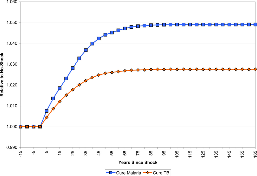
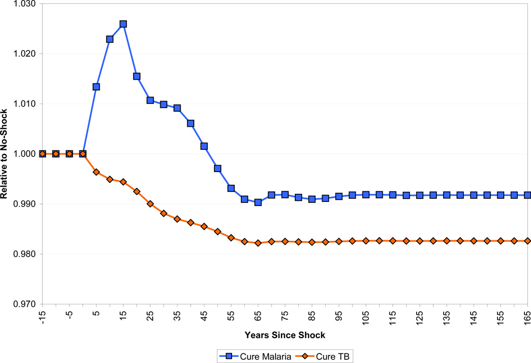
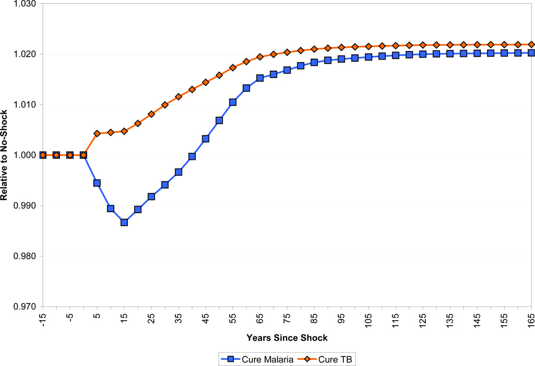
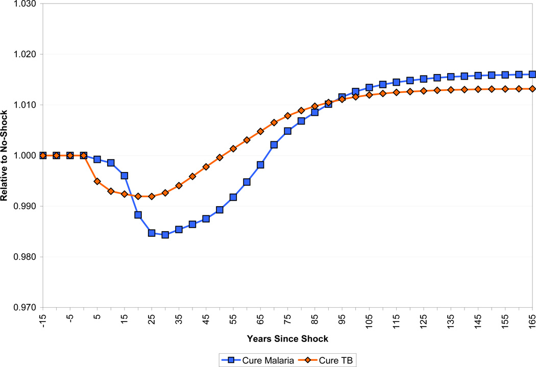
Figure 23 shows the paths of income per capita in the two eradication scenarios, compared to a baseline in which there is no change to health. The long-run effects are roughly similar: income per capita rises by 2 percent. The short-run paths are quite different, however. In the case of malaria eradication, income per capita initially dips to almost 1.5 percent below its pre-eradication level, and does not get back to its pre eradication level until some 40 years into the simulation. In the case of tuberculosis, by contrast, income rises immediately.

Figure 23.

Effect of Disease Eradication on Income per Capita

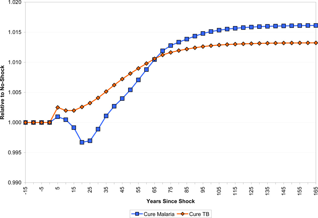
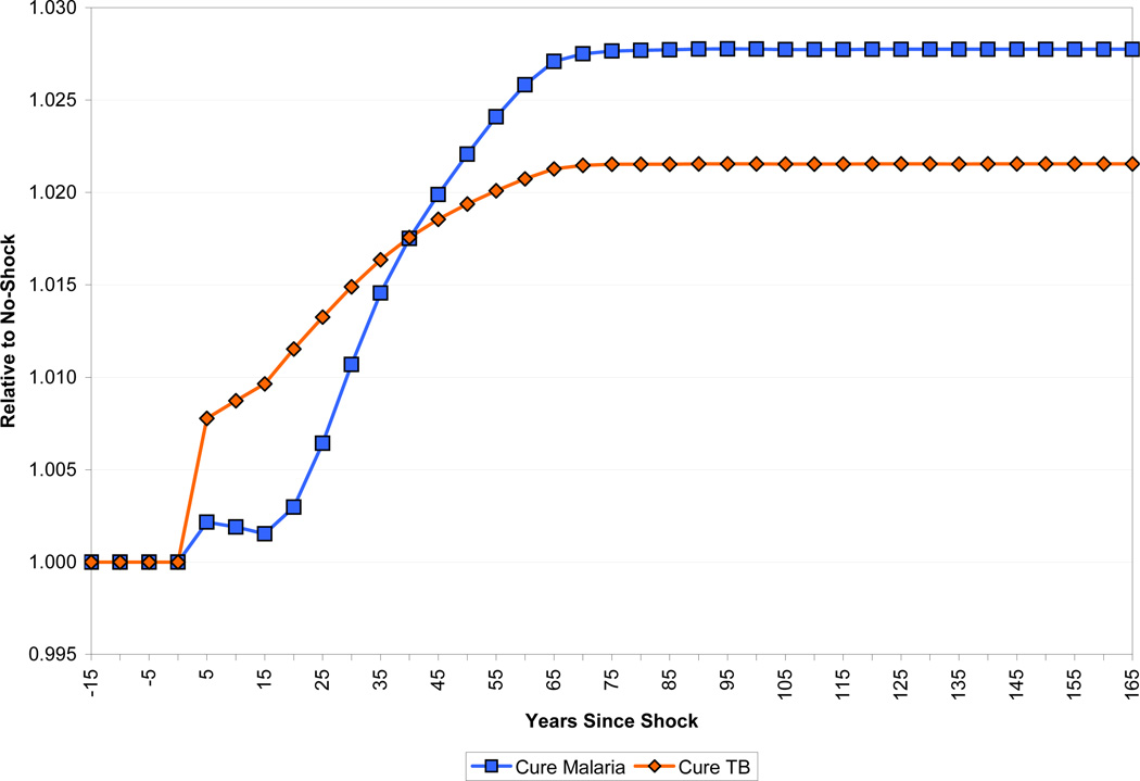
The differing demographic impact of the two diseases is part of the explanation for the divergent income paths. As Figure 24 shows, income per worker falls less in response to malaria eradication than does income per capita because of the increase in dependency that malaria eradication produces. In the long run, income per worker is higher for malaria eradication than in the case of tuberculosis eradication, but income per capita is equalized because the population with tuberculosis eradicated has a higher percentage of working-age adults. There are also interesting differences in the path of capital per worker, as shown in Figure 25. Capital per worker declines immediately in the case of tuberculosis eradication, since fewer working-age adults are dying. There is a larger, but more delayed decline in capital per worker in the case of malaria eradication as the cohort of children who would have died from the disease enter the labor force.

Figure 24.

Effect of Disease Eradication on Income per Worker

Figure 25.

Effect of Disease Eradication on Capital per Worker

The other source of the difference in the dynamic responses to eradication of malaria and tuberculosis is how they affect human capital. This is shown in Figure 26. In the case of tuberculosis, the biggest effect of eradication is on the productivity of workers. Table 2 shows that the prevalence of tuberculosis among adults is around 0.6 percent. Eradicating the disease immediately frees up this productive labor. By contrast, the prevalence of malaria episodes among adults is much lower, and eradicating malaria has only a delayed effect on the prevalence of neurological sequelae among adults. The part of the human capital increase that results from increased schooling, and thus takes a generation or more to phase in, is much higher for malaria. Malaria eradication raises schooling by 0.18 years, which accounts for most of the long-run increase in human capital from eradication. The increase in schooling from eradicating tuberculosis is only 0.09 years. Finally, eradicating tuberculosis reduces mortality mainly amongst prime-age workers, thereby skewing the age distribution of the population towards relatively more experienced workers. As a result, the long-run increase in human capital in the form of experience is about 4 times as great as that of eradicating malaria.

Figure 26.

Effect of Disease Eradication on Human Capital per Worker

Table 2.

Disease Burden for Females, Sub-Saharan Africa

Age	Incidence Rate (per 100,000)	Prevalence Rate (per 100,000)	Average Duration (years)	Death Rate (per 100,000)
	Malaria Episodes
0–4	120,000	1,644	0.01	559
5–14	17,500	240	0.01	42
15–44	17,500	240	0.01	33
45–59	17,500	240	0.01	36
	Malaria – Neurological Sequelae
0–4	164	365	37.1	0
5–14	0	701	-	-
15–44	0	617	-	-
45–59	0	474	-	-
	Tuberculosis (HIV sero-negative)
0–4	85	108	2.0	42
5–14	135	251	2.0	22
15–44	284	552	2.0	92
45–59	339	670	2.0	182

Source: Murray and Lopez (1996)

The most important things to note about our estimates is that the economic benefits of disease reduction are both small and, in the case of malaria, long in coming. These results stand in stark contrast to the assessments of the economic effects of malaria discussed in the introduction. The discussion of the sensitivity of our results to altering the parameterization of the model, conducted in Section Three in the case of general health improvement, can be carried over to this examination of individual diseases. Changing our assumptions about land’s role in production, the openness of the economy to capital flows, and the speed of fertility adjustment can increase the estimated benefits of disease reductions, but not by enough to match the estimates quoted above.

As we did for the general improvement in health analyzed earlier in the paper, we can examine the effect of disease eradication under a “best case” set of parameters that maximize (within reason) the effect of health on income per capita.¹¹ The results are shown in Figure 27. For malaria, income per capita returns to its baseline level after 25 years, rather than 40 years in the base case, and the total rise is 3 percent, versus 2 percent in the base case. The results for tuberculosis are qualitatively similar. Even in this best case, our results show an economic effect of disease eradication that is quite small.

Figure 27.

The Best Case Scenario for Income per Capita with Disease Eradication

As in our analysis of the effect of a general improvement in health, not every possible channel by which malaria or tuberculosis affect the economy is included in our analysis. In the case of malaria, two effects that are often mentioned are, first, reductions in agricultural productivity that result from farmers choosing land and/or crops in order to avoid exposure to the disease, and second, the effect of even low levels of disease in preventing some industries, most notably tourism, from getting started in a region. Beyond this, it may be that frequent absences produced by malaria result in a reduction in productivity that is greatly out of proportion to the number of days lost. We do not have good ways of incorporating any of these effects into our simulations.

5 Concluding Remarks

Using a simulation model, we explore the economic effects of an exogenous change in population health. The model allows for a direct effect of health on worker productivity, as well as indirect effects that run through schooling, the size and age-structure of the population, capital accumulation, and crowding of fixed natural resources. We also model the dynamic processes of phase-in of health improvements and the adjustment of fertility to a change in mortality that accompanies better health. Our analysis shows that for reasonable parameters, the period before any beneficial effects of an improvement in health are visible in GDP per capita can be quite long, on the order of a third of a century. It may take twice that long to achieve most of the long-run gains in income per capita resulting from increased health. Further, these gains are surprisingly small. An increase in life expectancy at birth from 40 to 60, in our base case simulation, raises GDP per capita by roughly 15 percent in the long run. When we examine the economic effects of eradicating specific diseases, we get similar results: eliminating either malaria or tuberculosis in the typical country in sub-Saharan Africa would raise GDP per capita by only two percent in the long run.

Our simulation model is parameterized using a combination of microeconomic estimates of the effect of health on schooling and worker productivity, data on demographics and disease burdens in developing countries, aggregate measures of the natural resource share in national income, and standard components of quantitative macroeconomic theory. The paper discusses how variations in the parameterization of the economic environment affect our results. No reasonable variation that we could come up with produces economic gains from health improvements of the magnitude that are commonly found in policy discussions of this issue.

The long lag with which health affects income per capita, along with the relatively modest long-run effect, may explain one of the more puzzling phenomena regarding cross-country inequality. While cross-country inequality in health declined rapidly over the period 1950–1990 (that is, up through the advent of the AIDS epidemic), cross-country inequality in income did not.

The results from our analyses of health’s effect on economic growth will have a number of uses. Considerations of economic effects are already an important part of discussions of and advocacy for programs to improve population health. While health improvements may well raise worker productivity, many potential interventions in developing countries will also be accompanied by the side effect of a rapidly growing population, which will have negative economic effects over a significant time horizon. An understanding of the demographic dynamics that accompany health improvements therefore suggests complementary policies and investments. Encouraging foreign investment may help mitigate capital dilution arising from population pressure. Planning for extra teachers and extra schooling facilities to cope with a likely large increase in the number of school-age children would mitigate adverse effects of crowding on human capital accumulation. Similarly, family-planning policies involving education or the availability of modern contraceptive methods are likely to limit the extent of population growth. Policies such as these can greatly improve the rate at which improvements in health are translated into improvements in the standard of living.

It is appropriate, though, to end on a note of caution. That improvements in health may temporarily (or even permanently) reduce income per capita is not a reason not to pursue such improvements, which are valuable in themselves. Similarly, family-planning policies need to be considered in the context of welfare analysis rather than simply through the lens of their effects on income per capita. This study is therefore complementary to the consideration of the welfare analysis of development policies, not a substitute for it.

References

- Acemoglu Daron, Johnson Simon. “Disease and Development: The Effect of Life Expectancy on Economic Growth”. Journal of Political Economy. 2007 Dec;115(6):925–985. [Google Scholar]
- Bils Mark, Klenow Peter J. “Does Schooling Cause Growth?”. American Economic Review. 2000 Dec;90(5):1160–1183. [Google Scholar]
- Bleakley Hoyt. “Disease and Development: Evidence from Hookworm Eradication in the American South”. Quarterly Journal of Economics. 2007a Feb;122(1):73–117. doi: 10.1162/qjec.121.1.73. [DOI] [PMC free article] [PubMed] [Google Scholar]
- Bleakley Hoyt. “Malaria in the Americas: A Retrospective Analysis of Childhood Exposure”; Chicago GSB. Working Paper; 2007b. [DOI] [PMC free article] [PubMed] [Google Scholar]
- Bloom David E, Canning David, Fink Günther, Finlay Jocelyn E. “Fertility, Female Labor Force Participation, and the Demographic Dividend”; Working Paper, Harvard School of Public Health.2007. [Google Scholar]
- Case Anne, Paxson Christina, Ableidinger Joseph. “Orphans in Africa: Parental Death, Poverty, and School Enrollment”. Demography. 2004 Aug;41(3):483–508. doi: 10.1353/dem.2004.0019. [DOI] [PubMed] [Google Scholar]
- Caselli Francesco, Feyrer James. “The Marginal Product of Capital”. Quarterly Journal of Economics. 2007 May;122(2):535–568. [Google Scholar]
- Cleland John. “The Effects of Improved Survival on Fertility: A Reassessment”. Population and Development Review. 2001;27(Supplement: Global Fertility Transition):60–92. [Google Scholar]
- Commission on Macroeconomics and Health. Macroeconomics and Health: Investing in Health for Economic Development. Geneva: World Health Organization; 2001. [Google Scholar]
- Deaton Angus. “Saving and Growth”. In: Schmidt-Hebbel Klaus, Servén Luis., editors. The Economics of Saving and Growth: Theory, Evidence, and Implications for Policy. New York, NY: Cambridge University Press; 1999. pp. 33–70. [Google Scholar]
- Fortson Jane G. “Mortality Risk and Human Capital Investment: The Impact of HIV/AIDS in Sub-Saharan Africa”. mimeo: University of Chicago; 2007. [Google Scholar]
- Hall Robert E, Jones Charles I. “Why Do Some Countries Produce So Much More Output Per Worker Than Others?”. Quarterly Journal of Economics. 1999 Feb;114(1):83–116. [Google Scholar]
- Hansen Gary D, Prescott Edward C. “Malthus to Solow”. American Economic Review. 2002 Sep;92(4):1205–1217. [Google Scholar]
- Kalemli-Ozcan Sebnem. “Does Mortality Decline Promote Economic Growth?”. Journal of Economic Growth. 2002 Dec;7(4):411–439. [Google Scholar]
- Kalemli-Ozcan Sebnem. “AIDS, ‘Reversal’ of the Demographic Transition and Economic Development: Evidence from Africa”. NBER Working Paper No. 12181.2008. [Google Scholar]
- Kalemli-Ozcan Sebnem, Ryder Harl E, Weil David N. “Mortality Decline, Human Capital Investment, and Economic Growth”. Journal of Development Economics. 2000 Jun;62(1):1–23. [Google Scholar]
- Keyfitz Nathan, Flieger Wilhelm. World Population: An Analysis of Vital Data. Chicago, IL: University of Chicago Press; 1968. [Google Scholar]
- Lee Ronald D, Mason Andrew, Miller Tim. “Saving, Wealth and Population”. In: Birdsall Nancy, Kelley Allen C, Sinding Steven W., editors. Population Matters: Demographic Change, Economic Growth, and Poverty in the Developing World. New York, NY: Oxford University Press; 2001. pp. 137–164. [Google Scholar]
- Lucas Adrienne M. “The Impact of Disease Eradication on Fertility and Education”. mimeo: Wellesley College; 2007a. [Google Scholar]
- Lucas Adrienne M. “The Impact of Malaria Eradication on Zambian Fertility: A Multigenerational Projection”. mimeo: Wellesley College; 2007b. [Google Scholar]
- Murray Christopher JL. “Rethinking DALYs”. In: Murray Christopher JL, Lopez Alan D., editors. The Global Burden of Disease: A Comprehensive Assessment of Mortality and Disability from Diseases, Injuries and Risk Factors in 1990 and Projected to 2020. Cambridge, MA: Harvard University Press; 1996. pp. 1–98. [Google Scholar]
- Murray Christopher JL, Lopez Alan D. The Global Burden of Disease: A Comprehensive Assessment of Mortality and Disability from Diseases, Injuries and Risk Factors in 1990 and Projected to 2020. Cambridge, MA: Harvard University Press; 1996. [Google Scholar]
- Nordhaus William D, Tobin James. “Is Growth Obsolete?,” in “Economic Growth, Economic Research: Retrospect and Prospect, Fiftieth Anniversary Colloquium, Vol. V, General Series No. 96”. New York, NY: Colombia University Press (for NBER); 1972. [Google Scholar]
- United Nations. Model Life Tables for Developing Countries. New York, NY: United Nations Population Division; 1982. [Google Scholar]
- Weil David N. “Accounting for the Effect of Health on Economic Growth”. Quarterly Journal of Economics. 2007 Aug;122(3):1265–1306. [Google Scholar]
- World Bank. Where is the Wealth of Nations? Measuring Capital for the 21st Century. Washington, DC: World Bank; 2005. [Google Scholar]
- Young Alwyn. “The Gift of the Dying: The Tragedy of AIDS and the Welfare of Future African Generations”. Quarterly Journal of Economics. 2005 May;120(2):423–466. [Google Scholar]
- Young Alwyn. “In Sorrow to Bring Forth Children: Fertility Amidst the Plague of HIV”. Journal of Economic Growth. 2007 Dec;12(4):283–327. [Google Scholar]