

Abstract
The additive genetic variance–covariance matrix (G) summarizes the multivariate genetic relationships among a set of traits. The geometry of G describes the distribution of multivariate genetic variance, and generates genetic constraints that bias the direction of evolution. Determining if and how the multivariate genetic variance evolves has been limited by a number of analytical challenges in comparing G-matrices. Current methods for the comparison of G typically share several drawbacks: metrics that lack a direct relationship to evolutionary theory, the inability to be applied in conjunction with complex experimental designs, difficulties with determining statistical confidence in inferred differences and an inherently pair-wise focus. Here, we present a cohesive and general analytical framework for the comparative analysis of G that addresses these issues, and that incorporates and extends current methods with a strong geometrical basis. We describe the application of random skewers, common subspace analysis, the 4th-order genetic covariance tensor and the decomposition of the multivariate breeders equation, all within a Bayesian framework. We illustrate these methods using data from an artificial selection experiment on eight traits in Drosophila serrata, where a multi-generational pedigree was available to estimate G in each of six populations. One method, the tensor, elegantly captures all of the variation in genetic variance among populations, and allows the identification of the trait combinations that differ most in genetic variance. The tensor approach is likely to be the most generally applicable method to the comparison of G-matrices from any sampling or experimental design.
Keywords: genetic variance, G-matrix, tensor, Bayesian, MCMC
Introduction
The distribution of genetic variation among multiple traits is a key determinant of how a population will respond to selection (Lande, 1979; Schluter, 1996; Arnold et al., 2001). For the prediction of evolutionary responses, the genetic variation in multiple traits is described by the symmetrical genetic variance–covariance matrix, G (Lande, 1980; Phillips and McGuigan, 2006). Genetic variances, and particularly covariances, depend on underlying genetic details such as the frequencies of alleles and the distribution of their effect sizes (Barton and Turelli, 1987; Turelli, 1988; Turelli and Barton, 1990), and hence are subject to change under both drift and selection. It is therefore reasonable to expect that the genetic variance in multiple traits might differ among populations, and consequently that the responses of these populations to the same selective force might also differ.
Although determination of the genetic details underpinning G is an active research area (Kelly, 2009), the general lack of information on the distribution of allelic effects and frequencies currently makes it impossible for theoretical quantitative genetic models to clearly predict the evolutionary dynamics of G. Several studies have circumvented this problem through simulation-based approaches, exploring the impact of variation in parameters describing evolutionary processes (selection, mutation and migration) on the evolution of G (Jones et al., 2003, 2004; Guillaume and Whitlock, 2007; Jones et al., 2007; Revell, 2007). These studies have demonstrated that G will evolve to the greatest extent in small populations, under weak correlational selection on traits, through directional selection against major axes of G, and when mutational correlation among traits is low. Simulated parameter ranges are based on information from nature (see Arnold et al. (2008)), but nonetheless, we typically lack information on multivariate mutation and selection, and on migration in specific natural populations and for multivariate trait sets of interest. It remains an empirical question whether G typically varies among populations in ways that will impact on their future responses to selection.
Numerous empirical studies have taken a comparative approach to determine evolutionary rates, and the processes affecting G (Steppan et al., 2002; Arnold et al., 2008). Although G-matrices are highly conserved among some populations (see Arnold et al. (2008)), they have also been demonstrated to rapidly diverge among both natural populations and experimental treatments (Cano et al., 2004; Doroszuk et al., 2008; Hine et al., 2009; Johansson et al., 2012). Laboratory manipulations have demonstrated that G can evolve rapidly in response to drift (Phillips et al., 2001), and that selection can drive rapid and repeatable evolution of G (Blows and Higgie, 2003; Hine et al., 2011). Further, the reproduction by experimental evolution of patterns observed in G among natural populations (Blows and Higgie, 2003), and the observations that the strength (Hunt et al., 2007) and pattern (Roff and Fairbairn, 2012) of selection are associated with levels of genetic variation in populations suggest selection might have a discernible effect on G.
Logistical limitations on estimating quantitative genetic parameters, particularly the need for relatively large samples, have restricted the utility of comparative quantitative genetics. However, more generally, the identification and interpretation of the variation among G-matrices has been limited by the lack of an appropriate statistical framework, a long-standing and ongoing analytical challenge (Turelli, 1988; Steppan et al., 2002; Hansen and Houle, 2008; Marroig et al., 2011; Roff et al., 2012). Various properties of symmetrical matrices can be described by summary parameters such as their size (the trace), measures of their ill-conditioned nature or eccentricity (Jones et al., 2003; Kirkpatrick, 2009), and the correlation among matrix elements (Roff et al., 2012). More complex hypotheses concerning proportionality, and a series of partial trait combination (principal component) comparisons using a hierarchy of similarity can also be tested (Flury, 1988; Phillips and Arnold, 1999).
There are a number of drawbacks that are shared by many of these current approaches. First, the majority of methods use metrics that do not clearly relate to evolutionary theory (Hansen and Houle, 2008), making it difficult to connect divergence in G to simple changes in genetic variance and the response to selection. Second, comparisons are typically made in the absence of any specific information on the direction of selection, and information on selection cannot be readily incorporated into some metrics. Third, many approaches can be applied only to data derived from simple experimental designs and are not well suited for applications involving the more complex experimental designs typically employed in experimental evolution studies or replicated sampling from different environments in the field. Finally, approaches for comparing G are typically focused on differences between pairs of populations, with no simple generalisation to multi-population studies. We are therefore lacking an analytical approach that is generally applicable across the data structures typical of studies in experimental and natural populations, which can be used to provide statistical confidence in inferred differences, and which can be used to predict differences between populations in their ongoing evolution. Our aim in this paper is to provide a cohesive and general analytical framework for comparative quantitative genetics that incorporates and extends existing geometric approaches, as it is the geometry of G that generates evolutionary constraints and determines the extent to which particular traits will respond to a given episode of selection (Walsh and Blows, 2009).
The response of a population to a particular vector of selection gradients (β) for a set of n traits is given by (Lande, 1979):
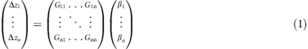 |
where G rotates (and scales) the response away from the direction of β, resulting in some level of genetic constraint (Walsh and Blows, 2009); the geometry of G determines the bias in the response to selection. Although individual traits feature as the rows and columns of G, it is important to realise that these individual measured traits do not necessarily have a greater role in the response to selection than any combination of the traits. Recognising G as simply characterising the level of genetic variance in all possible trait combinations (Blows and Hoffmann, 2005) provides a point of departure for the framework we outline in this paper for establishing how G differs among populations, and the evolutionary consequences of those differences.
To begin, consider how the genetic variance in any trait combination can be found using the projection (Lin and Allaire, 1977):
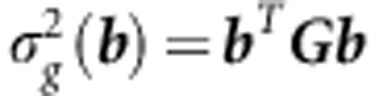 |
where b is scaled to unit length. It is the relative orientation of the direction of b to the distribution of genetic variance in G that determines how biased the response will be away from b when selection is applied in this direction. The distribution of genetic variances in G can be represented by the eigenvalues (λ) of G, that is, by the genetic variances of the orthogonal trait combinations described by the eigenvectors. Most estimated G tend to be ill-conditioned, displaying an exponential-like decay in λ (Kirkpatrick, 2009). The influence of the λi and its corresponding eigenvectors (gi) on the response to selection can be shown using a spectral decomposition of the multivariate breeders' equation (Walsh and Blows, 2009):
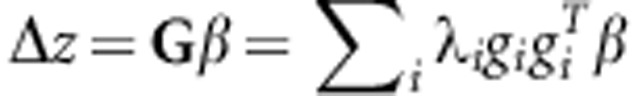 |
When genetic variation is much larger in some trait combinations than others (for example, the λ decay exponentially), there are two possible consequences for the response to selection that are not apparent from the consideration of single trait heritabilities and selection gradients. First, individual traits might respond to selection in the direction opposite to their selection gradient. Second, the set of correlated traits might respond overall in a direction that is substantially different from the direction of selection applied (that is, β). Both these possible outcomes become more likely as the magnitude of genetic variation becomes smaller in the direction of selection relative to other trait combinations (Walsh and Blows, 2009). Even if the direction of selection differs among populations, the pattern of phenotypic divergence might resemble the pattern of genetic covariation among traits more than the pattern of divergent selection if G is highly ill-conditioned, and the genetic variance is low in the directions of selection (Chenoweth et al., 2010).
In this paper, we bring together within a single statistical framework a number of geometrical approaches designed to establish differences in G-matrices among multiple populations. The approaches we consider are restricted to those that establish a change in genetic variance among populations rather than methods that focus on other matrix summary parameters that are not directly related to the response to selection. We integrate all approaches into a Bayesian framework that enables uncertainty to be placed on the estimation of differences among populations, and we provide worked examples for all approaches based on six G-matrices derived from a previously published data set. Finally, in the on-line Supplementary Material, we supply the R code (Dryad repository: doi:10.5061/dryad.g860v) for the programs and matrix manipulations needed to conduct these analyses.
Materials and methods
We develop four specific approaches to the comparison of G-matrices, all of which focus on establishing differences in genetic variance. The methods increase in complexity, from considering the level of genetic variance in random vectors and how these differences among matrices are distributed across the phenotypic space (Method 1), to the identification of higher-dimensional common spaces (Method 2) and ending with two approaches that consider differences in genetic variance across the entire space (Methods 3–4). The first three methods assume no more information is available than the G-matrices themselves, while Method 4 takes advantage of information on the direction of selection when it is known.
Bayesian analyses
We place all four approaches in a Bayesian framework that enables the estimation of uncertainty on the genetic parameters that are estimated. One particularly useful feature of Bayesian approaches for the comparison of G is that the uncertainty in estimates of nuisance parameters (for example, trait and generation means in the analyses presented below) is integrated out of the marginal posterior distributions of the parameters of interest (Gelman et al., 2004). The joint marginal posterior distributions therefore capture the uncertainty in G, but also any uncertainty in the estimates of the nuisance parameters influencing G.
Owing to the complexity of the models required to analyse data typical of evolutionary quantitative genetics studies, the full posterior distribution can often not be derived analytically. In these cases, however, it is possible to use Markov chain Monte Carlo (MCMC) methods to evaluate the posterior distribution (Gelman et al., 2004). Here, the Markov process is used to move the chain from a random starting value to regions of parameter space with greater density, thereby permitting sampling of the joint posterior distribution at each step in MCMC chain. When applied correctly, the combination of MCMC and Bayesian approaches allows us to evaluate the full posterior distribution of the parameters of interest while accounting for the uncertainty introduced by nuisance parameters. Furthermore, because the variation among samples of the marginal posterior distribution captures the uncertainty in estimates of the model parameters, applying any linear transformation (for example, projection of a linear combination through a G) to the samples of the posterior distributions preserves this uncertainty (O'Hara et al., 2008; Ovaskainen et al., 2008). Hence, the uncertainty can be carried forward into new analyses and to provide estimates of confidence for metrics of similarity or dissimilarity among matrices.
A useful characteristic of using MCMC approaches to evaluate the posterior distributions of the model parameters is that the variance components are constrained to be positive, and hence the estimated G matrices will be positive definite. Consequently, the posterior distribution of a variance component cannot be used to test whether the variance component is significantly different from zero. It is therefore important to construct a sensible null model for the hypothesis test of interest. For example, to examine whether an increase in the breeding values of Soay sheep on island of St Kilda reflected positive selection on breeding values, Hadfield et al. (2010) compared the observed temporal trend in breeding values with a null model representing the temporal tend in breeding values under genetic drift alone. Their study demonstrated that, despite the uncertainty in the estimated breeding values (as determined through Bayesian methods), the increase in the average breeding value of the Soay sheep population was greater than the null, and so it is likely that selection rather than drift caused the observed increase in breeding values.
Here, we use a similar approach to compare our observed differences among G-matrices to a null model where we assume the differences among G are driven by random sampling variation alone. Conceptually, our approach is equivalent to the standard approach of estimating null G through the randomisation of individuals (or families) among populations (Roff et al., 2012). The key difference here is that we generate the null G from the posterior predictive distribution of breeding values for the observed G. This approach has several general advantages. First, this approach can be applied across diverse pedigree structures where the unit of randomisation is the individual's estimated genetic value (Ovaskainen et al., 2008). Second, because the null G are estimated from the posterior predictive distribution of breeding values, the approach has a lower computational requirement than re-running models for each randomised data set. Finally, the procedure ensures that the set of randomised G-matrices have the same structure as the set of observed G-matrices. Consequently, the same matrix comparison metrics can be applied to both the observed and randomised G, allowing hypothesis tests comparing differences in our observed G to a set of null G, based on the assumption that differences are driven by sampling alone.
To generate our randomised G, we first estimate the marginal posterior distribution of G for our six populations of interest (described below). Second, for each MCMC sample, we calculate posterior predictive breeding values for individuals by taking draws from a multivariate normal distribution with a mean of zero and a variance of the ith MCMC sample of the jth G. Importantly, breeding values are assigned using the pedigree corresponding to each population. Finally, we randomly assign individuals to one of six hypothetical populations and construct G-matrices from the vectors of breeding values.
Example data set
The example data set we use is a subset of an experiment reported in Hine et al. (2011), where specific details of the experimental design and laboratory procedures can be found. Briefly, an artificial selection experiment was conducted on eight traits (cuticular hydrocarbons) in Drosophila serrata. There were two treatments (b and m) in which different linear combinations of the eight traits were selected on for 11 generations, with two replicate populations per treatment. Two control (c) populations were also maintained under the same experimental conditions. In both of the treatments, and in the controls, paternal pedigrees were recorded for all males every generation, and the eight traits were recorded for each of these males. Here, we utilised the pedigree and phenotypic data from the final four generations (8–11) to estimate G using an animal model. This yielded a total of six G-matrices for comparison. The G for each population was estimated using the MCMCglmm package (Hadfield, 2010) in R (R Development Core Team, 2013) to fit the model:
 |
where X, Z1 and Z2 are the incidence matrices that, respectively, relate the vectors of trait and generation means (b), the vector of additive genetic effects (u1) and the vector of vial effects (u2) to the observations in y. The vector e contains the error. MCMCglmm fits mixed models in a Bayesian framework using MCMC to sample the posterior distributions of the location effects and variance components. For the location parameters, priors were normally distributed and diffuse about a mean of zero and a variance of 108. For the variance components, we used weakly informative inverse-Wishart priors with the parameters for the distribution set to 0.001 for the degrees of freedom, and for the scale parameter we defined a diagonal matrix containing values of one third of the phenotypic variance. To assist with model convergence, the response vector (y) was rescaled, with all elements multiplied by 10. The joint posterior distribution was estimated from 1 003 000 MCMC iterations sampled at 100 iteration intervals after an initial burn-in period of 3000 iterations. Overall, model convergence (Geweke as well as Gelman and Rubin diagnostics) and model fit diagnostics (posterior predictive distributions) indicated the MCMC chain sampled the parameter space adequately. Example script to run these models is presented in Dryad (Dryad repository: doi:10.5061/dryad.g860v). The functions for the matrix comparison methods below are presented in the Supplementary material as a tutorial and in Dryad (Dryad repository doi: 10.5061/dryad.g860v).
Method 1. Random projections through G
Random skewers is a method used to compare differences in orientation among G (Cheverud, 1996; Cheverud and Marroig, 2007). In these approaches, random β vectors are placed into the multivariate breeders' equation with each G, and the vector correlations between the resulting Δz vectors are used as an indication of the differences among G. The test for the significance of the similarity or dissimilarity of the matrices is then evaluated by comparison of the distribution of observed vector correlations with a distribution of vector correlations conforming to a null model. The null models are often generated by bootstrapping and represent cases where matrices have coincident spaces (vector correlations of∼1) (for example, Calsbeek and Goodnight (2009)), or cases where matrices have distinct spaces (vector correlations of ∼0) (for example. Cheverud and Marroig (2007)), depending on whether researchers are interested in convergence or divergence among G (Roff et al., 2012).
Hansen and Houle (2008) described how, in addition to the differences in Δz, a random skewer approach can be used to examine differences among G in the magnitude of genetic variance (as well as metrics of variance such as evolvability and respondability) using matrix projection. In this section, we develop an approach based on the projection of random skewers that, when used in combination with estimates of marginal posterior distribution of G, can test for differences in the magnitude of genetic variances. This approach can also be used to describe the trait combinations that differ most often among G. Although we limit our approach here to differences in genetic variance among matrices, it is readily adapted to other scaled measures of variance such as evolvability and respondability.
Each random vector (typically 1000 or more) is projected through each MCMC sample of each G-matrix to generate a posterior distribution of the genetic variance in the direction of the random vector for each population. Differences in genetic variance among populations are then evaluated by examining the overlap of the highest posterior density (HPD) intervals between all possible combinations of populations. All vectors that result in non-overlapping HPD intervals between any pair of populations are then collated, and the product-moment G of the vector elements calculated. This n × n matrix (where n is the number of traits), R, describes which parts of the phenotypic space tend to show significant differences in genetic variance and this part of the space can be further investigated through an eigenanalysis of R. It is important to note that, because the random skewers probe the entire phenotypic space, each significant random skewer (that is, the vectors contributing to the estimation of R) can contain some component of those dimensions that significantly differ, as well as of those that do not. Therefore, to identify which dimensions of R represent genuine differences in genetic variance, we projected the eigenvectors of R back onto both the observed and randomised G-matrices.
Method 2. Krzanowski's common subspaces
The most basic, and perhaps the most important, question one can ask about multivariate genetic variance is: which part of the trait space has genetic variance, and which part does not? To answer this question, approaches to determining the dimensionality of G have been developed, defining that subspace of G for which there is statistical evidence for the existence of genetic variance (Kirkpatrick and Meyer, 2004; Meyer and Kirkpatrick, 2005; Mezey and Houle, 2005; Hine and Blows, 2006). When multiple populations are present, the identification of which subspace is shared among G is necessarily complicated because of the many different hypotheses that are possible to test. Krzanowski (1979) first described how to establish if the parts of the space that contain ‘most' of the (genetic) variation are similar between two (G) matrices using:
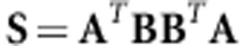 |
where the matrices A and B contain a subset k of the eigenvectors of the two G as columns, and where k⩽n/2. The sum of the eigenvalues of S gives a bounded statistic, which ranges between complete orthogonality (0) and complete overlap (k) of the two subspaces, respectively. Blows et al. (2004) give further details on the use of this approach for comparing G-matrices and second-order fitness surfaces.
For more than two populations, the subspace most similar across populations (t=1, …, p) is found using (Krzanowski, 1979):
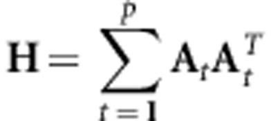 |
where At contains the subset kt of the eigenvectors (as columns) of Gt. The first k (k=min(ki), i=1,…, p) eigenvalues of H can take on a maximum value of p. Any eigenvector of H associated with an eigenvalue equal to p can be reconstructed exactly for a given population from a linear combination of the eigenvectors of G that defined that population's subspace for the calculation of H. Eigenvalues less than p indicate that at least one population cannot exactly reconstruct the corresponding eigenvector of H from a linear combination of the eigenvectors of G that defined its subspace. For those eigenvalues less than p, we can quantify how close the corresponding eigenvector of H is to each population's subspace.
The angle (δ) between each eigenvector of H and each of the p population subspaces is given by:
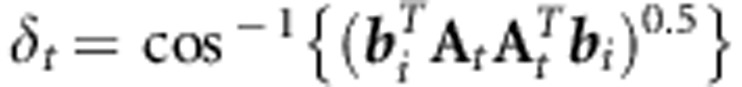 |
Although Krzanowski's approach identifies common subspaces based on their orientation, the magnitude of genetic variance contained in even identical subspaces could vary substantially. For instance, differences in total matrix size, or variation among G in eigenvector order could lead to differences among populations in the genetic variance associated with a common subspace. Insight into differences among populations in genetic variance associated with common subspaces can be gained in this context by using projection to find the genetic variance in each population for those bi that are judged to form part of the common subspace. Statistically significant differences among matrices in the magnitude of the genetic variation in the common space can then be determined using the overlap among HPD intervals.
It is worth noting here the relationship between Krzanowski's approach, and the more comprehensive hierarchy of common space comparisons developed by Flury (1988). Although Krzanowski's approach is directed towards determining if those eigenvectors explaining the most variance are similar, the Flury hierarchy imposes no such restriction. For most applications in quantitative genetics, Krzanowski's approach is likely to have the greater utility for two reasons. First, as shown by equation (1), it is that part of the space of G that contains the most genetic variance that determines the extent of bias in the response to selection, and therefore how differently populations might respond to the same selection regime. Second, the Flury method was developed for product-moment covariance matrices, and hence the degrees of freedom to properly implement the full Flury hierarchy are unknown for all but the most simple of genetic designs requiring variance-component estimation of G. Application of the Flury method to the comparative analysis of G is therefore strictly limited.
Method 3. The genetic covariance tensor
We now describe an approach that is designed to determine how matrices differ without recourse to the random probing of the matrices as in method 1 above. For the simple case of a comparison of two matrices, two similar approaches have been used to determine if the matrices are different. The first is the resultant matrix of the difference, C=A−B; and recently a likelihood ratio tests of the rank of the difference have been developed (Schott, 2010). In the evolutionary literature, the comparison of G-matrices through their difference forms the basis of approaches exploring how much divergence between populations can be caused by uniform linear selection (Hansen and Houle, 2008), and also to assist in identifying dimensions for univariate comparisons of genetic variance (Sztepanacz and Rundle, 2012). The second metric is the resultant matrix of the ratio C=A−1B. This metric forms the basis of the comparisons of phenotypic covariance matrices in the morphometrics literature (Mitteroecker and Bookstein, 2009). For both of these approaches, the leading eigenvectors of the resultant matrix, C, reveal which dimensions differ most between the two matrices, on the absolute scale in the first instance or on the relative scale in the second.
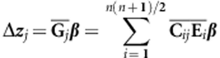
A natural extension of the comparison of two matrices by analysing their difference is the characterization of the variation among multiple matrices with the fourth-order covariance tensor, Σ (Hine et al., 2009). The order of a tensor indicates how many indices are required to reference its elements; for example, vectors and matrices are first and second-order tensors, respectively. A fourth-order tensor is required to describe the variation among multiple matrices. The eigenanalysis of a covariance tensor (discussed in detail below) calculated on two matrices returns the matrix of the difference between two matrices. The elements of Σ represent the variances of, and covariances among, the elements of the multiple covariance matrices:
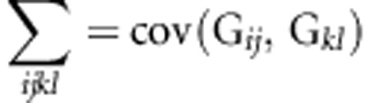 |
Obtaining E, the set of  second-order eigentensors of Σ, is the first step in
exploring the variation among matrices that is summarized by Σ. The
eigentensors and eigenvalues of Σ are analogous to the eigenvectors and
eigenvalues of a product-moment G in several ways. First, the eigentensors
describe independent aspects of variation in covariance structure, the same way
eigenvectors describe uncorrelated dimensions of variation in trait space. Second, the
original G-matrices can each be expressed as a linear combination of the eigentensors,
the same way a given vector can be expressed as a linear combination of eigenvectors.
Third, the size of the eigenvalue corresponding to an eigentensor reflects the variation
among matrices with respect to how much that eigentensor contributes to their covariance
structure. Fourth, the maximum number of non-zero eigenvalues of a covariance tensor is
equal to the smaller of
second-order eigentensors of Σ, is the first step in
exploring the variation among matrices that is summarized by Σ. The
eigentensors and eigenvalues of Σ are analogous to the eigenvectors and
eigenvalues of a product-moment G in several ways. First, the eigentensors
describe independent aspects of variation in covariance structure, the same way
eigenvectors describe uncorrelated dimensions of variation in trait space. Second, the
original G-matrices can each be expressed as a linear combination of the eigentensors,
the same way a given vector can be expressed as a linear combination of eigenvectors.
Third, the size of the eigenvalue corresponding to an eigentensor reflects the variation
among matrices with respect to how much that eigentensor contributes to their covariance
structure. Fourth, the maximum number of non-zero eigenvalues of a covariance tensor is
equal to the smaller of  and p−1, the same way the maximum number of non-zero eigenvalues of a
covariance matrix is the smaller of n and the sample size minus one. In
practice, the eigentensors of Σ can be obtained by first mapping
Σ onto the symmetric
and p−1, the same way the maximum number of non-zero eigenvalues of a
covariance matrix is the smaller of n and the sample size minus one. In
practice, the eigentensors of Σ can be obtained by first mapping
Σ onto the symmetric  matrix S (Figure 1; see Hine et al. (2009) for details). The elements of the
ith eigenvector of S can then be scaled and arranged to form
Ei.
matrix S (Figure 1; see Hine et al. (2009) for details). The elements of the
ith eigenvector of S can then be scaled and arranged to form
Ei.
Figure 1.

Matrix representation of a fourth-order tensor. The top-left quadrant of the matrix contains the (co)variances of the variances (for example, Σii, kk). The bottom-right quadrant of the matrix contains the (co)variances of the covariances (for example, Σij, kl). Finally, the upper-right and lower-left quadrants contain the covariances of the variances and covariances (for example, Σii, kl).
The next step in exploring the variation among matrices summarized by Σ is to obtain the eigenvectors and eigenvalues of the eigentensors, which can be interpreted in a similar way to those of G. For example, if the largest eigenvalue of an eigentensor is close to 1, the detected change in covariance structure can be attributed to the change in genetic variance in a single trait combination. Unlike a true covariance matrix, eigentensors can have a mix of positive and negative eigenvalues, which will result when a co-ordinated change in genetic variance involves an increase in genetic variance in some trait combinations and a decrease in others.
The Bayesian framework can be utilised to determine which of the independent aspects of
genetic covariance structure identified by the tensor exhibit significant variation
among populations. First, for the ith MCMC sample of the set of G, we
determine the matrix respresentation of the tensor, Si. Next,
we calculate the elements of  from the corresponding posterior means of the elements of the set
of Si (i=1 to 10 000). The
jth eigenvector of
from the corresponding posterior means of the elements of the set
of Si (i=1 to 10 000). The
jth eigenvector of  is then projected onto Si
(equivalent to projecting
is then projected onto Si
(equivalent to projecting  onto Σ) to determine
αij, the variance among the ith
MCMC sample of the G-matrices for the aspect of covariance structure specified by
onto Σ) to determine
αij, the variance among the ith
MCMC sample of the G-matrices for the aspect of covariance structure specified by
 . Projecting an
eigentensor onto a tensor is analogous to projecting a vector onto a G-matrix to
determine how much variance is present in a particular direction. The posterior
distribution of αj summarizes the uncertainty
in the variance in covariance structure represented by
. Projecting an
eigentensor onto a tensor is analogous to projecting a vector onto a G-matrix to
determine how much variance is present in a particular direction. The posterior
distribution of αj summarizes the uncertainty
in the variance in covariance structure represented by  . This distribution of
αj is then compared with a distribution of
the αj generated from the null model, where
the variation among matrices is due to sampling variation, not biologically meaningful
differences.
. This distribution of
αj is then compared with a distribution of
the αj generated from the null model, where
the variation among matrices is due to sampling variation, not biologically meaningful
differences.
Method 4. The decomposition of the multivariate breeders' equation
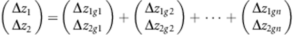
The approaches discussed so far are generally applicable in the sense that no further biological information is required other than the G themselves. However, in the presence of information on the direction of selection, more specific hypotheses concerning how differences among G bias the response to selection can be addressed. For a single population, equation (1) can be re-written to emphasize the responses of the individual traits. For example, in a two trait analysis, (1) can be written as:
 |
In this form, it can be seen how the ith eigenvector of G (gi) contributes a proportion of the response for each of the individual traits. The magnitude of this contribution is determined by how close β is to that particular eigenvector, and how large its eigenvalue is. Using this decomposition in an empirical setting, the differences between two populations in their response to the same β can be partitioned into differences as a result of each eigenvector of G.
Uncertainty can be placed on the predicted multivariate response to selection using the genetic covariance between fitness and the metric traits included in the analysis. This approach incorporates uncertainty both in the estimation of G and in the vector of selection gradients β. However, for many biological systems, measures of fitness (and thus the estimates of selection) might typically come from experiments that are independent of the breeding designs used to estimate G. Here, we therefore consider only the situation where uncertainty in the response to selection, and how G influences this response, is a product of uncertainty in G itself and not in β.
For any pair of populations, a difference in overall predicted response for an individual trait can be determined from the comparison of HPD intervals of the linear transformation by β of the posterior samples of G. To determine which eigenvectors of G have contributed to this difference, we use a slightly modified version of equation (1). Here, we substitute λi in equation (1) with the genetic variance for each MCMC sample of G in the direction of the eigenvectors of posterior mean G. This allows us to generate the posterior distribution of eigenvector-specific components of the predicted response for each population.
An alternative way to view the effects of differences in G on the response to selection is to focus on the major changes in genetic variance among the G matrices. This can be achieved by using an alternative decomposition of the breeders' equation that involves the eigentensors of the genetic covariance tensor:
 |
where  is the
Frobenius inner product of
is the
Frobenius inner product of  and
and  and reflects the weighting of the ith eigentensor for the jth
posterior mean. Then, similar to our modification to equation (1) above, we can generate
the posterior distribution of
and reflects the weighting of the ith eigentensor for the jth
posterior mean. Then, similar to our modification to equation (1) above, we can generate
the posterior distribution of  as the set of Frobenius inner products of
  in each MCMC sample of
Gj.
in each MCMC sample of
Gj.
Results
Method 1. Random projections through G
If we treat our G-matrices as a set of unstructured populations (randomly sampled geographic populations, for example), there are 15 pairwise comparisons that indicated significant differences in genetic variance between populations. Of the 1000 random skewers, 166 have non-overlapping 95% HPD intervals for at least one pairwise comparison of genetic variances for our six populations, a typical example of which is displayed in Figure 2a (compare with Figure 2b). To characterise the orientation of these 166 significant random vectors, we then calculated their G (R). The projection of the eigenvectors of R on the set of observed G revealed that only the first eigenvector of R resulted in non-overlapping HPD intervals for at least one pairwise comparison of genetic variances (r1 in Table 1). The leading eigenvector of R represented a trait combination that has a high genetic variance in one of the m populations (Supplementary Table S1a). We note that this eigenvector closely resembles the trait combination captured by the leading eigenvector of the second eigentensor in method 3 (vector correlation=0.94; Table 1).
Figure 2.

Results from method 1. (a) An example of a random vector that identified a significant difference in additive genetic variation among populations. (b) An example of a random vector that resulted in overlapping posterior distributions of additive genetic variation among populations.
Table 1. Summary of vectors representing matrix comparison metrics.
| r 1 | h 1 a | h 1 b | e 11 | e 21 | |
|---|---|---|---|---|---|
| lc2 | 0.506 | −0.087 | −0.088 | −0.095 | 0.247 |
| lc3 | −0.825 | −0.082 | −0.090 | −0.075 | −0.949 |
| lc4 | −0.214 | −0.064 | −0.064 | −0.099 | −0.137 |
| lc5 | 0.008 | −0.218 | −0.214 | −0.148 | −0.062 |
| lc6 | 0.071 | −0.204 | −0.207 | −0.238 | 0.072 |
| lc7 | 0.063 | −0.285 | −0.285 | −0.302 | −0.037 |
| lc8 | 0.009 | −0.828 | −0.827 | −0.807 | −0.090 |
| lc9 | −0.092 | −0.356 | −0.353 | −0.393 | −0.023 |
lc2—lc9 are the log-contrasts of the ratios to Z,Z-5,9-C24:2 of, respectively: Z,Z-5,9-C25:2, Z-9-C25:1, Z-9-C26:1, 2-Me-C26, Z,Z-5,9-C27:2, 2-Me-C28, Z,Z-5,9-C29:2, 2-Me-C30. See Hine et al. (2011) for full details of these traits.
r1 is the first eigenvector of the R matrix for an unstructured experimental design. h1a and h1b are the first eigenvectors of H for our two examples (first four eigenvectors and eigenvectors capturing 90% of observed variance, respectively). e11 and e21 are the first eigenvectors of the first and the second eigentensors, respectively.
In our example, the six G-matrices represent three treatment groups, each with two replicate populations. The posterior distributions of the replicate populations can be combined, and differences among treatments identified in the same fashion as outlined above. Thus, if we re-analyse our data, acknowledging the underlying experimental design, at 95% HPD, none of the 1000 vectors differed significantly in genetic variance between the b and c treatments, whereas 90 differed between the m and c treatments. At 90% HPD, this increased to 8 and 129 vectors, for the comparisons of b vs c and c vs m, respectively. Unsurprisingly, the first eigenvector of R for the 90% HPD comparison of the b and c treatments shows a similarity with the leading eigenvector of the first eigentensor in method 3 (vector correlation=0.64) and describes an increase in genetic variance in the b treatments (Supplementary Table S1b). The first eigenvector of R for the 90% HPD comparison of the c and m treatments captured significantly more variance in the m treatments (Supplementary Table S1c), and was almost identical with the first eigenvector of R for the analysis of the six populations without consideration of the experimental design.
Method 2. Krzanowski's common subspaces
There are two ways one could approach determining the presence of a common subspace among the G using Krzanowski's H. The first includes a fixed number of eigenvectors for each G, while the second allows the number of eigenvectors included for each matrix to differ. In the first example analysis, we used the first four eigenvectors of each G, while in the second example, we included the number of eigenvectors required to account for at least 90% of the genetic variance in the posterior mean G of each population. To determine if the subspaces of our observed G were shared among the six populations, we looked for a significant departure from the null hypothesis of a common set of principal components. This is analogous to testing if a genetic correlation is significantly different from one, rather than zero.
The first four eigenvectors of G explained at least 81% of the genetic variance in each of the six populations. The first two eigenvalues of H estimated from these subspaces approached the maximum value of 6 for this specific case, while the next two eigenvalues dropped to below 5 and 4, respectively. However, for all four interpretable eigenvectors of H (h1 to h4), the 95% HPD intervals overlapped those of the null model, indicating that we had no evidence for these subspaces having diverged among the populations (Figure 3a). Inspection of the angles (Supplementary Table S2a) between the first four eigenvectors of H and the AtAtT subspaces of our observed set of G-matrices supported this conclusion: the 95% HPD intervals for the angles of the first four eigenvectors of H overlapped for all populations.
Figure 3.

Results from method 2. (a) Eigenvalues of H for a comparison of the first four eigenvectors of each G matrix. (b) Eigenvalues of H for a comparison of the minimum number of eigenvalues required to account for 90% of the variation of the posterior mean observed G. Shaded regions of the plots indicate eigenvectors of H > min(ki).
Our second example application of Krzanowski's common subspaces ensured that we captured at least 90% of the genetic variance in each G. Figure 3b shows that the eigenvalues of this second H are very similar to those of our first example (see also Supplementary Table S2b). However, compared with the first example, we observed a slower decay in size of the eigenvalues of H, and that the uncertainty surrounding these eigenvalues was also reduced. This suggests that allowing the distributions of variance in G to dictate the eigenvectors to include uncovered greater similarity among the set of G-matrices.
Method 3. The genetic covariance tensor
With six populations, the genetic covariance tensor will have at most five non-zero eigenvalues. The 95% HPD intervals of α for the non-zero eigenvalues of the genetic covariance tensor suggested that only E2 described significant variation among the observed G. At 90% HPD, however, we found that posterior distribution of α for the first two eigentensors (E1 and E2) of the observed and null sets of G-matrices were non-overlapping, indicating marginal support for the variation among G described by E1 (Figure 4a). The eigenanalyses of these eigentensors revealed that the leading eigenvectors of E1 and E2 accounted for 73% and 70% of the variation in these eigentensors, respectively. Projection of e11 and e21 onto the observed G-matrices indicated that the change in genetic variance captured in e11 was driven by the two b populations, while in e21 the change in genetic variance was attributable to a single m population (Figures 4b, c). Both of these vectors are associated with those identified by the random projection analysis (Table 1; Supplementary Table S1a-b). e21 was found to be almost coincident with the first eigenvector of R from the among-population random projection analysis, while e11 was similar to the first eigenvector of R from the among-treatment analysis, with weakly significant differences between the b and c treatments.
Figure 4.

Results from method 3. (a) Variance accounted for by each eigentensor (α) for the observed G and the null G. (b, c) The additive genetic variance in each population in the direction of e11 and e21, respectively.
Method 4. The decomposition of the multivariate breeders' equation
The vector of directional sexual gradients was determined in the base population of the selection experiment (Iss in Hine et al. (2011)). Using this as our estimate of β in the multivariate breeders' equation, we determined if there was any significant difference between any pair of the populations in the predicted response to selection of any individual traits. Two traits, lc2 and lc6, displayed at least one significant difference in response (Figures 5a, b; Supplementary Table S3a), indicating that the differences in G among populations are predicted to result in different evolutionary responses. In both cases, at least one of the b populations was shown to be different from the c2 population as a result of the divergence in G identified by the analyses above.
Figure 5.

Results from method 4. (a,b) The posterior means and 95% HPD intervals for the predicted response to selection for each population for the two traits (lc2 and lc6) for which there were significant among-population differences in Δz (indicated by asterisk). (c, d) The contribution of gmax to differences in Δz for lc2 and lc6 in the populations where Δz differed significantly. (e,f) The contribution of the remaining eigenvectors of G to the predicted differences in responses to selection. Note the change in scale for the y axis between c, d vs e, f.
Decomposition of the breeders' equation into the response to selection along each of the eigenvectors of G showed that the predicted differences in the lc2 and lc6 traits among populations were mostly due to differences in gmax (Figures 5c–f). The tendency for a bias in the predicted response in the direction of gmax is because of the magnitude of the eigenvalue of gmax relative to the other vectors (Chenoweth et al., 2010). Closer examination of the orientation of gmax in each population revealed that the significant differences in the selection response were due to changes in orientation of gmax, which evolved to reflect the sizeable increases of genetic variance in the direction of e11 and e21 in the b treatments (that is, b1 and b2 populations) and the m2 population, respectively.
Differences attributable to E1 were not significant (Supplementary Table S3a), a somewhat surprising result given that a difference in genetic variance between b and c2 populations is associated with E1 (method 3 results), and the significant differences in predicted response between these populations (described above). This apparent inconsistency can be explained by the differences in the uncertainty associated with estimating genetic variance in the various trait combinations represented by gmax across the six populations (for example Figures 5c, d). This uncertainty is sufficiently large to ensure the sizeable change in genetic variance in e11 between the posterior mean G-matrices for the b populations resulted in overlapping posterior density intervals. In contrast, the uncertainty in estimating the genetic variance in the trait combination represented by gmax in c2 is sufficiently small that the difference between this population and one of the b populations is significant (Figure 5c). Finally, significant differences as a consequence of the change in genetic variance captured by E2 were predicted for the response of all traits in the pairwise comparisons of population m2 with the m1, c1 and c2 populations (Supplementary Table S3b).
Discussion
Although many approaches have been developed for comparisons of G-matrices, the majority of these approaches suffer from limitations either in the evolutionary hypotheses that can be addressed (Hansen and Houle, 2008), or in the types of experimental designs to which they can be applied (Roff et al., 2012). Furthermore, the interpretation of results is not always clear (Houle et al., 2002), and the application of different approaches to the same data has revealed that different methods often do not agree on whether the matrices are considered similar or not (Calsbeek and Goodnight, 2009; Roff et al., 2012).
There are three particular attributes of the approaches we have detailed here that go some way to addressing these issues. First, our goal in this paper has been to supply a series of approaches that facilitate the biological interpretation of variation in G. All approaches focus on a change in genetic variance, rather than other metrics that attempt to describe more holistic ways in which matrices may differ (for example, proportionality, equality or matrix correlation). This is important because it is ultimately the level of genetic variance in particular directions that result in the biologically important consequences of differences in G, such as influencing the response to selection (Chenoweth et al., 2010), or the evolution of genetic variance itself (Hine et al., 2011).
Second, we have chosen a robust and flexible statistical framework within which all methods can be accommodated. The Bayesian framework carries through the uncertainty known to be associated with estimates of genetic variance and directly incorporates this uncertainty into determining if the distribution of multivariate genetic variance differs among populations. This framework can be used for pedigreed populations, as in our example, or for more traditional breeding designs. In addition to accommodating any experimental design, our approaches can be readily modified to include genetic variances measured on different scales; the evolvability and respondability of Hansen and Houle (2008), for example.
Finally, although each of these methods concentrates on different aspects of the distribution of the genetic variance within populations, the analyses should be able to be interpreted in a consistent manner. In our worked example, the differences found by the random skewers approach were supported by the partitioning of differences in genetic variance among populations using the covariance tensor. Nonetheless, the Krzanowski subspace comparisons revealed that the majority of genetic variance for the six populations was still found in the coincident space. The final approach, using the decomposition of the breeders' equation, showed how differences among G alter the predicted response selection, and emphasised that differences in the response are biased in the direction of greatest genetic variation.
Although we have shown here how both the tensor and random skewers approaches consistently identify the trait combinations that differ in genetic variance, it is likely that the tensor will be the most direct and efficient approach to determining how a set of G differ. All the variation among the G-matrices is captured concisely by the genetic covariance tensor, allowing the direct identification of trait combinations that differ in the magnitude of their genetic variance. Non-orthogonal trait combinations can even be identified if their changes in genetic variance are uncorrelated across populations. In contrast, the random skewers approach relies on a summary of the random trait combinations that differ in genetic variance among populations to infer a subset of the multivariate genetic variance that differs in genetic variance, defined by orthogonal trait combinations. It is therefore a much less precise or direct approach than the tensor.
Analyses of how G-matrices differ among populations can easily become mired down in the vast number and variety of hypotheses that could potentially be tested. By focusing on differences in genetic variance, and how those differences are distributed within the phenotypic space, it is possible to generate a consistent picture of how G vary among populations, and the effect such differences will have on the response to selection. Combined with the flexible nature of Bayesian approaches for placing uncertainty on complex metrics, the analyses we describe provide a comprehensive solution to the complex problem of characterizing differences among G sampled from any experimental design.
Data archiving
Cuticular hydrocarbon and pedigree data, and example R code have all been deposited at Dryad (Dryad repository: doi:10.5061/dryad.g860v).
Acknowledgments
We thank J Kelly, B Walsh and one anonymous reviewer for comments that significantly improved the manuscript. We thank T Godsen for comments that improved the tutorial. This research was funded by the Australian Research Council.
The authors declare no conflict of interest.
Footnotes
Supplementary Information accompanies this paper on Heredity website (http://www.nature.com/hdy)
Supplementary Material
References
- Arnold SJ, Burger R, Hohenlohe PA, Ajie BC, Jones AG. Understanding the evolution and stability of the G-matrix. Evolution. 2008;62:2451–2461. doi: 10.1111/j.1558-5646.2008.00472.x. [DOI] [PMC free article] [PubMed] [Google Scholar]
- Arnold SJ, Pfrender ME, Jones AG. The adaptive landscape as a conceptual bridge between micro- and macro-evolution. Genetica. 2001;112:9–32. [PubMed] [Google Scholar]
- Barton NH, Turelli M. Adaptive landscapes, genetic distance and the evolution of quantitative characters. Gen Res. 1987;49:157–173. doi: 10.1017/s0016672300026951. [DOI] [PubMed] [Google Scholar]
- Blows MW, Chenoweth SF, Hine E. Orientation of the genetic variance-covariance matrix and the fitness surface for multiple male sexually selected traits. Am Nat. 2004;163:E329–E340. doi: 10.1086/381941. [DOI] [PubMed] [Google Scholar]
- Blows MW, Higgie M. Genetic constraints on the evolution of mate recognition under natural selection. Am Nat. 2003;161:240–253. doi: 10.1086/345783. [DOI] [PubMed] [Google Scholar]
- Blows MW, Hoffmann AA. A reassessment of genetic limits to evolutionary change. Ecology. 2005;86:1371–1384. [Google Scholar]
- Calsbeek B, Goodnight CJ. Empirical comparison of G matrix test statistics: Finding biologically relevant change. Evolution. 2009;63:2627–2635. doi: 10.1111/j.1558-5646.2009.00735.x. [DOI] [PubMed] [Google Scholar]
- Cano JM, Laurila A, Palo J, Merila J. Population differentiation in G matrix structure due to natural selection in Rana temporaria. Evolution. 2004;58:2013–2020. doi: 10.1111/j.0014-3820.2004.tb00486.x. [DOI] [PubMed] [Google Scholar]
- Chenoweth SF, Rundle HD, Blows MW. The contribution of selection and genetic constraints to phenotypic divergence. Am Nat. 2010;175:186–196. doi: 10.1086/649594. [DOI] [PubMed] [Google Scholar]
- Cheverud JM. Quantitative genetic analysis of cranial morphology in the cotton-top (Saguinus oedipus) and saddle-back (S. fuscicollis) tamarins. J Evol Biol. 1996;9:5–42. [Google Scholar]
- Cheverud JM, Marroig G. Comparing covariance matrices: random skewers method compared to the common principal components model. Genet Mol Biol. 2007;30:461–469. [Google Scholar]
- Doroszuk A, Wojewodzic MW, Gort G, Kammenga JE. Rapid divergence of genetic variance-covariance matrix within a natural population. Am Nat. 2008;171:291–304. doi: 10.1086/527478. [DOI] [PubMed] [Google Scholar]
- Flury B. Common Principal Components and Related Multivariate Models. Wiley: New York, NY, USA; 1988. [Google Scholar]
- Gelman A, Carlin JB, Stern HS, Rubin DR. Bayesian Data Analysis. Chapman & Hall/ CRC: Boca Raton, Florida, USA; 2004. [Google Scholar]
- Guillaume F, Whitlock MC. Effects of migration on the genetic covariance matrix. Evolution. 2007;61:2398–2409. doi: 10.1111/j.1558-5646.2007.00193.x. [DOI] [PubMed] [Google Scholar]
- Hadfield JD. MCMC methods for multi-response generalized linear mixed models: The MCMCglmm R package. J Stat Software. 2010;33:1–22. [Google Scholar]
- Hadfield JD, Wilson AJ, Garant D, Sheldon BC, Kruuk LEB. The misuse of BLUP in ecology and evolution. Am Nat. 2010;175:116–125. doi: 10.1086/648604. [DOI] [PubMed] [Google Scholar]
- Hansen TF, Houle D. Measuring and comparing evolvability and constraint in multivariate characters. J Evol Biol. 2008;21:1201–1219. doi: 10.1111/j.1420-9101.2008.01573.x. [DOI] [PubMed] [Google Scholar]
- Hine E, Blows MW. Determining the effective dimensionality of the genetic variance–covariance matrix. Genetics. 2006;173:1135–1144. doi: 10.1534/genetics.105.054627. [DOI] [PMC free article] [PubMed] [Google Scholar]
- Hine E, Chenoweth SF, Rundle HD, Blows MW. Characterizing the evolution of genetic variance using genetic covariance tensors. Phil Trans R Soc Lond B Biol Sci. 2009;364:1567–1578. doi: 10.1098/rstb.2008.0313. [DOI] [PMC free article] [PubMed] [Google Scholar]
- Hine E, McGuigan K, Blows MW. Natural selection stops the evolution of male attractiveness. Proc Natl Acad Sci USA. 2011;108:3659–3664. doi: 10.1073/pnas.1011876108. [DOI] [PMC free article] [PubMed] [Google Scholar]
- Houle D, Mezey J, Galpern P. Interpretation of the results of common principal components analyses. Evolution. 2002;56:433–440. doi: 10.1111/j.0014-3820.2002.tb01356.x. [DOI] [PubMed] [Google Scholar]
- Hunt J, Blows MW, Zajitschek F, Jennions MD, Brooks R. Reconciling strong stabilizing selection with the maintenance of genetic variation in a natural population of black field crickets (Teleogryllus commodus) Genetics. 2007;177:875–880. doi: 10.1534/genetics.107.077057. [DOI] [PMC free article] [PubMed] [Google Scholar]
- Johansson F, Lind MI, Ingvarsson PK, Bokma F. Evolution of the G-matrix in life history traits in the common frog during a recent colonisation of an island system. Evol Ecol. 2012;26:863–878. [Google Scholar]
- Jones AG, Arnold SJ, Burger R. Stability of the G-matrix in a population experiencing pleiotropic mutation, stabilizing selection, and genetic drift. Evolution. 2003;57:1747–1760. doi: 10.1111/j.0014-3820.2003.tb00583.x. [DOI] [PubMed] [Google Scholar]
- Jones AG, Arnold SJ, Burger R. Evolution and stability of the G-matrix on a landscape with a moving optimum. Evolution. 2004;58:1639–1654. doi: 10.1111/j.0014-3820.2004.tb00450.x. [DOI] [PubMed] [Google Scholar]
- Jones AG, Arnold SJ, Burger R. The mutation matrix and the evolution of evolvability. Evolution. 2007;61:727–745. doi: 10.1111/j.1558-5646.2007.00071.x. [DOI] [PubMed] [Google Scholar]
- Kelly JK. Connecting QTLs to the G-matrix of evolutionary quantitative genetics. Evolution. 2009;63:813–825. doi: 10.1111/j.1558-5646.2008.00590.x. [DOI] [PMC free article] [PubMed] [Google Scholar]
- Kirkpatrick M. Patterns of quantitative genetic variation in multiple dimensions. Genetica. 2009;136:271–284. doi: 10.1007/s10709-008-9302-6. [DOI] [PubMed] [Google Scholar]
- Kirkpatrick M, Meyer K. Direct estimation of genetic principal components: simplified analysis of complex phenotypes. Genetics. 2004;168:2295–2306. doi: 10.1534/genetics.104.029181. [DOI] [PMC free article] [PubMed] [Google Scholar]
- Krzanowski WJ. Between groups comparision of principal components. J Am Stat Assoc. 1979;74:703–707. [Google Scholar]
- Lande R. Quantitative genetic analysis of multivariate evolution, applied to brain:body size allometry. Evolution. 1979;33:402–416. doi: 10.1111/j.1558-5646.1979.tb04694.x. [DOI] [PubMed] [Google Scholar]
- Lande R. The genetic covariances between characters maintained by pleiotropic mutations. Genetics. 1980;94:203–215. doi: 10.1093/genetics/94.1.203. [DOI] [PMC free article] [PubMed] [Google Scholar]
- Lin CY, Allaire FR. Heritability of a linear combination of traits. Theor Appl Genet. 1977;51:1–3. doi: 10.1007/BF00306054. [DOI] [PubMed] [Google Scholar]
- Marroig G, Melo D, Porto A, Sebastiao H, Garcia G. Selection response decomposition (SRD): a new tool for dissecting differences and similarities between matrices. Evol Biol. 2011;38:225–241. [Google Scholar]
- Meyer K, Kirkpatrick M. Restricted maximum likelihood estimation of genetic principal components and smoothed covariance matrices. Genet Sel Evol. 2005;37:1–30. doi: 10.1186/1297-9686-37-1-1. [DOI] [PMC free article] [PubMed] [Google Scholar]
- Mezey JG, Houle D. The dimensionality of genetic variation for wing shape in Drosophila melanogaster. Evolution. 2005;59:1027–1038. [PubMed] [Google Scholar]
- Mitteroecker P, Bookstein F. The ontogenetic trajectory of the phenotypic covariance matrix, with examples from craniofacial shape in rats and humans. Evolution. 2009;63:727–737. doi: 10.1111/j.1558-5646.2008.00587.x. [DOI] [PubMed] [Google Scholar]
- O'Hara RB, Cano JM, Ovaskainen O, Teplitsky C, Alho JS. Bayesian approaches in evolutionary quantitative genetics. J Evol Biol. 2008;21:949–957. doi: 10.1111/j.1420-9101.2008.01529.x. [DOI] [PubMed] [Google Scholar]
- Ovaskainen O, Cano JM, Merila J. A Bayesian framework for comparative quantitative genetics. Proc R Soc B Biol Sci. 2008;275:669–678. doi: 10.1098/rspb.2007.0949. [DOI] [PMC free article] [PubMed] [Google Scholar]
- Phillips PC, Arnold SJ. Hierarchical comparison of genetic variance-covariance matrices. I. Using the Flury hierarchy. Evolution. 1999;53:1506–1515. doi: 10.1111/j.1558-5646.1999.tb05414.x. [DOI] [PubMed] [Google Scholar]
- Phillips PC, McGuigan K.Evolution of genetic variance covariance structure (G)In: Fox CW, Wolf JB, (eds.)Evolutionary Genetics: Concepts and Case Studies Oxford University Press: Oxford, UK; 310–325.2006 [Google Scholar]
- Phillips PC, Whitlock MC, Fowler K. Inbreeding changes the shape of the genetic covariance matrix in Drosophila melanogaster. Genetics. 2001;158:1137–1145. doi: 10.1093/genetics/158.3.1137. [DOI] [PMC free article] [PubMed] [Google Scholar]
- R Development Core Team . R Foundation for Statistical Computing: Vienna, Austria; 2003. [Google Scholar]
- Revell LJ. The G matrix under fluctuating correlational mutation and selection. Evolution. 2007;61:1857–1872. doi: 10.1111/j.1558-5646.2007.00161.x. [DOI] [PubMed] [Google Scholar]
- Roff DA, Fairbairn DJ. The evolution of trade-offs under directional and correlational selection. Evolution. 2012;66:2461–2474. doi: 10.1111/j.1558-5646.2012.01634.x. [DOI] [PubMed] [Google Scholar]
- Roff DA, Prokkola JM, Krams I, Rantala MJ. There is more than one way to skin a G matrix. J Evol Biol. 2012;25:1113–1126. doi: 10.1111/j.1420-9101.2012.02500.x. [DOI] [PubMed] [Google Scholar]
- Schluter D. Adaptive radiation along genetic lines of least resistance. Evolution. 1996;50:1766–1774. doi: 10.1111/j.1558-5646.1996.tb03563.x. [DOI] [PubMed] [Google Scholar]
- Schott JR. Reduced-rank estimation of the difference between two covariance matrices. J Stat Plan Infer. 2010;140:1038–1043. [Google Scholar]
- Steppan SJ, Phillips PC, Houle D. Comparative quantitative genetics: evolution of the G matrix. Trends Ecol Evol. 2002;17:320–327. [Google Scholar]
- Sztepanacz JL, Rundle HD. Reduced genetic variance among high fitness individuals: Inferring stabilizing selection on male sexual displays in Drosophila serrata. Evolution. 2012;66 (10:3101–3110. doi: 10.1111/j.1558-5646.2012.01658.x. [DOI] [PubMed] [Google Scholar]
- Turelli M. Phenotypic evolution, constant covariances, and the maintenance of additive variances. Evolution. 1988;42:1342–1347. doi: 10.1111/j.1558-5646.1988.tb04193.x. [DOI] [PubMed] [Google Scholar]
- Turelli M, Barton NH. Dynamics of polygenic characters under selection. Theor Popul Biol. 1990;38:1–57. [Google Scholar]
- Walsh B, Blows MW. Abundant genetic variation+strong selection=multivariate genetic constraints: A geometric view of adaptation. Annu Rev Ecol Evol Syst. 2009;40:41–59. [Google Scholar]
Associated Data
This section collects any data citations, data availability statements, or supplementary materials included in this article.