Recovery of sparse translation-invariant signals with continuous basis pursuit

Abstract

We consider the problem of decomposing a signal into a linear combination of features, each a continuously translated version of one of a small set of elementary features. Although these constituents are drawn from a continuous family, most current signal decomposition methods rely on a finite dictionary of discrete examples selected from this family (e.g., shifted copies of a set of basic waveforms), and apply sparse optimization methods to select and solve for the relevant coefficients. Here, we generate a dictionary that includes auxiliary interpolation functions that approximate translates of features via adjustment of their coefficients. We formulate a constrained convex optimization problem, in which the full set of dictionary coefficients represents a linear approximation of the signal, the auxiliary coefficients are constrained so as to only represent translated features, and sparsity is imposed on the primary coefficients using an L1 penalty. The basis pursuit denoising (BP) method may be seen as a special case, in which the auxiliary interpolation functions are omitted, and we thus refer to our methodology as continuous basis pursuit (CBP). We develop two implementations of CBP for a one-dimensional translation-invariant source, one using a first-order Taylor approximation, and another using a form of trigonometric spline. We examine the tradeoff between sparsity and signal reconstruction accuracy in these methods, demonstrating empirically that trigonometric CBP substantially outperforms Taylor CBP, which in turn offers substantial gains over ordinary BP. In addition, the CBP bases can generally achieve equally good or better approximations with much coarser sampling than BP, leading to a reduction in dictionary dimensionality.

I. Introduction

The decomposition of signals into sparse linear combinations of features is an important and well-studied problem, and plays a central role in many applications. A surge of recent effort focuses on representing a signal as a noisy superposition of the smallest possible subset of features drawn from a large finite dictionary. However, many real signals are generated by processes that obey natural invariances (e.g., translation-invariance, dilation-invariance, rotation-invariance). For example, the acoustic features of many sounds can occur at arbitrary times, dilations, or frequencies. In photographic images, features can occur at various spatial locations, scales, and orientations. Radar [1] and seismic [2] signals are often composed of elementary features that are translated and frequency-modulated. For these signals, a desirable goal is to identify features in the signal along with their associated amplitudes and transformation parameters.

In the majority of published examples, this problem is solved by constructing a finite dictionary that reflects the invariant structure: one discretely samples the transformation parameters and applies these to a finite set of elementary features. For example, dictionaries for sound processing, whether hand-constructed or learned, are commonly “convolutional”, containing time-delayed copies of template waveforms (e.g., [3], [4], [5]). Dictionaries for image representation typically contain features that are translated, and in some cases, dilated and rotated (e.g., [6], [7], [8], [9]).¹ Using this finite dictionary {φ_i(t)}, one then attempts to optimize the corresponding coefficients:

$$\underset{\overline{x}\in {\mathbb{R}}^d}{min}{\Vert \overrightarrow{x}\Vert }_0,\text{s}.\text{t}.{\Vert y(t)-\sum _{i=1}^d{x}_i{\phi }_i(t)\Vert }_2\le \epsilon ,$$ (1)

where y(t) is a noisy observation, x⃗ is a coefficient vector, ε bounds the L₂ norm of the noise, and ||·||₀ indicates the L₀ pseudonorm (number of nonzero elements). In general, this objective can only be minimized via exhaustive search of all 2^d subsets of the dictionary, making it infeasible in practice. However, two broad classes of approximate solutions have been widely studied in the literature. The first consists of greedy methods, dating back to variable selection methods in the 1970s ([13]). These methods are exemplified by the well-known “matching pursuit” algorithm of Mallat and Zhang [14], and include a variety of more recent “iterative thresholding” methods [15], [16], [17], [18], [19]. The general idea is to solve sequentially for the nonzero coefficients, at each step choosing the dictionary element(s) that best explain the current residual. The second category of solutions arises from convex relaxations of Eq. (1), which typically employ the L₁ norm [20], [21].

The use of a finite dictionary allows one to approximate the full nonlinear problem with a more tractable linear inverse problem. However, the ability of this discrete dictionary to compactly represent signals depends critically on the spacing at which the dictionary is sampled. In general, a very fine sampling is required, resulting in a very large and ill-conditioned dictionary. This ill-conditioning, in turn, is unfavorable for the approximation methods mentioned above. Furthermore, it is unclear how to estimate the underlying amplitudes and transformation parameters from the coefficients.

Here, we propose an alternative linear approximation to the full nonlinear problem. We focus on the problem of translation-invariant, one-dimensional signals (although the methods generalize to other transformations, and higher dimensions). We construct a group of functions that can span local translations of the feature templates via continuous variation of their coefficients (as a concrete example, consider the original templates and their derivatives, which can approximate local translations through a first-order Taylor approximation). A signal of interest is then represented in this dictionary by “block-sparse” coefficients, where each non-zero coefficient block represents an amplitude-scaled and translated template. We formulate an objective function in which the coefficients are constrained so as to only represent scaled/transformed templates, and use an L₁ penalty to impose sparsity on the blocks. The advantage of this approach over ordinary BP is three-fold: (1) better approximation of translation-invariant signals, (2) a smaller basis, which leads to sparser solutions via convex optimization, and (3) an explicit mapping from this representation to amplitudes and transformation parameters. An early version of this work was presented in [22].

II. Problem formulation

We begin by formulating a simple generative model for translation-invariant signals, as well as the maximum-aposteriori (MAP) estimation framework for inferring the most likely parameters given the observed signal. Assume we observe a signal that is a noisy superposition of scaled time-shifted copies of a single known elementary waveform f(t) on a finite interval [0, T]:

$$y(t)=\sum _{j=1}^N{a}_{j}f(t-{\tau }_j)+\eta (t),$$ (2)

where η(t) is a Gaussian white noise process with power σ², the event times {τ_j} are a Poisson process with rate μ, and the event amplitudes {a_j} are drawn independently from a density P_A(a). The inverse (inference) problem is to recover the most likely parameters {τ_j, a_j} given y(t). This amounts to maximizing the posterior distribution P ({τ_j, a_j}|y(t)), which reduces, on taking the negative log, to solving:

$$\underset{\begin{array}{c}N,\{a_j\}\\ \{{\tau }_1<\dots <{\tau }_N\}\end{array}}{min}\frac{1}{2{\sigma }^2}{\Vert y(t)-\sum _{j=1}^N{a}_{j}f(t-{\tau }_j)\Vert }_2^2-Nlog(\mu )-\sum _{j=1}^{N}log{P}_A(a_j)$$ (3)

Unfortunately, solving Eq. (3) directly is intractable, due to the discrete nature of N and the nonlinear embedding of the τ_j’s within the argument of the waveform f(·). It is thus desirable to find alternative formulations that (i) approximate the signal posterior distribution well, (ii) have parameters that can be tractably estimated, and (iii) have an intuitive mapping back to the original representation.

III. Conventional solution: discretization and BP

A standard simplification of the problem is to discretize the event times at a spacing that is fine enough that the Poisson process is well-approximated by a Bernoulli process. The interval [0, T] is divided into N_Δ = ⌈T/Δ⌉ time bins of size Δ, and μΔ approximates the probability of an event in each bin.² This discrete process is represented by a vector x⃗ ∈ ℝ^N_Δ, whose elements x_i are interpreted as the amplitude of any event in the interval ( $\frac{(2i-1)\mathrm{\Delta }}{2},\frac{(2i+1)\mathrm{\Delta }}{2}$). The corresponding prior probability distribution on each x_i is a mixture of a point mass at zero, and P_A(·):

$$P(\overrightarrow{x})=\prod _{i=1}^{N_{\mathrm{\Delta }}}[(1-\mu \mathrm{\Delta })\delta (x_i)+(\mu \mathrm{\Delta })P_A(x_i)]$$ (4)

By taking the log and applying standard approximations, the MAP estimation for this model can be approximated by:

$$\underset{\overrightarrow{x}}{min}\frac{1}{2{\sigma }^2}{\Vert y(t)-(F_{\mathrm{\Delta }}\overrightarrow{x})(t)\Vert }_2^2-log(\mu \mathrm{\Delta }){\Vert \overrightarrow{x}\Vert }_0-\sum _{i:x_i\ne 0}log{P}_A(x_i)$$ (5)

where F_Δ is a linear operator representing a fixed dictionary of time-shifted copies of f(·):

$$(F_{\mathrm{\Delta }}\overrightarrow{x})(t):=\sum _{i=1}^{N_{\mathrm{\Delta }}}{x}_{i}f(t-i\mathrm{\Delta }).$$ (6)

The advantage of the time discretization is that the data fidelity term is now a quadratic function of the parameters. Despite this, solving Eq. (5) exactly is NP-hard due to the L₀ term [23], and so we must either resort to approximate algorithms, or introduce further approximations in the objective. A well-known convex relaxation (known as the LASSO [20] or basis pursuit denoising [21]) replaces the nonconvex prior terms in Eq. (5) with an L₁ penalty term, resulting in:

$$\underset{\overrightarrow{x}}{min}\frac{1}{2{\sigma }^2}{\Vert y(t)-(F_{\mathrm{\Delta }}\overrightarrow{x})(t)\Vert }_2^2+\lambda {\Vert \overrightarrow{x}\Vert }_1$$ (7)

where λ > 0 is a parameter to be determined. This was previously applied in the convolutional setting, for example in [24], [25]. Note that probabilistically, the second term indicates that we have effectively approximated the nonconvex mixture prior of Eq. (4) with a Laplacian distribution, P (x) ∝ e^−λ|x|.

The global optimum of Eq. (7) can be found using standard quadratic programming methods. A well-known article by Candès et al. [26] provides sufficient conditions under which L₁-minimizing solutions are good approximations for L₀-minimizing solutions (up to a term that is linear in the L₂ norm of the noise). Roughly speaking, the condition limits the correlations between small subsets of dictionary elements. However, this condition is rarely satisfied in the convolutional setting (even when f is smooth) because the validity of the discrete approximation typically requires Δ to be quite small, resulting in a highly correlated dictionary F_Δ. In addition to these concerns about the tradeoff between the quality of discrete approximation and the convex relaxation, the discretization of time also leaves us with no well-defined mapping between the solution of Eq. (5) and the continuous parameters {τ_j, a_j} that optimize the original objective of Eq. (3).

One can understand the extent of these problems more concretely by focusing on a single time-shifted waveform f(t − τ) with τ ∈ (0, Δ), and a dictionary containing the feature at two gridpoints: F_Δ = [f (t), f (t − Δ)]. Equation (7) is then a 2D problem, as illustrated in Fig. 2(a). The optimal solution corresponds to a point at which an elliptical level curve of the first (L₂) term is tangent to a straight-line level curve of the L₁ term. Note that the ellipses are stretched in the direction parallel to the L₁ level lines, because trading off amplitude between the two coefficients does not substantially change the reconstruction error when Δ is small (specifically, one can show mathematically that the two right singular vectors of the basis matrix are parallel and orthogonal to the L₁ level curves). Also shown in Fig. 2(a) is the family of solutions that are obtained as λ varies from 0 to +∞ (red path). Notice that these solutions are not sparse in the L₀ sense (i.e., they do not intersect either of the two axes) until λ is so large that the signal reconstruction is quite poor. This is the case regardless of how small Δ is, and is due both to the failure of the L₁ norm to approximate the L₀ pseudonorm and to the inability of the discrete model to account for continuous event times. In the following sections, we develop and demonstrate a proposed solution for these problems.

Fig. 2.

Geometry of convex objective functions for BP, CBP-T, and CBP-P methods, illustrated in two dimensions. Signal consists of a single waveform, f(t − 0.65Δ), and the dictionary contains two shifted copies of the waveform, {f(t), f(t − Δ)}, along with interpolating functions appropriate for each method. Each plot shows the space of coefficients, {x₁, x₂}, associated with the two shifted waveforms. Contours of gray-scale regions indicate level surfaces of reconstruction error (L₂ norm term of the objective function). The blue star indicates the true L₀-minimizing solution. The L₁ sparsity measure is the sum of the two coefficient values, corresponding to the vertical position on the plot. Red curve indicates family of solutions traced out as λ is increased from 0 (yellow dot) to infinity. Red points along this path indicate equal increments in reconstruction accuracy, with enlarged point indicating a common value for comparison across all three methods. (a) Standard BP solution (Eq. (7)). (b) Continuous basis pursuit with Taylor interpolator (Eq. (13)), using a basis of {f₀, $f_0^{\prime }$, f_Δ, $f_{\mathrm{\Delta }}^{\prime }$}. In this case, the iso-accuracy contours are computed by minimizing the L₂ error over all feasible values of the derivative coefficients, and are thus no longer elliptical. (c) CBP with polar interpolation (Eq. (20)).

IV. Continuous basis pursuit

The motivation for the discretization of the inference problem was tractability. Equation (5) approximates the original model well in the limit as Δ goes to 0, but it is only tractably solvable in regimes where Δ is large enough so that correlations are limited and L₁-based relaxations can be employed. In this section, we augment the discrete model by incorporating variables to account for the continuous nature of the event times, and adapt the LASSO to solve this augmented representation. By accounting for continuous time-shifts, the augmented model not only approximates the original model better (and for a larger range of Δ), but also admits sparser solutions via an L₁-based recovery method. We refer to this method as continuous basis pursuit (CBP).

We return to the original formulation of Eq. (3), but we assume (without loss of generality) that the waveform is normalized, ||f(t)||₂ = 1, and that the amplitudes, {a_j}, are all nonnegative. Our noisy observation arises from a linear superposition of time-shifted waveforms, f(t − τ) abbreviated as f_τ (t). The set of all time-shifted and amplitude-scaled waveforms constitute a nonlinear 2D manifold:

$${\mathcal{M}}_{f,T}:=\{{af}_{\tau }(t):a\ge 0,\tau \in [0,T]\}\subset L_2([0,T]).$$ (8)

The discretized dictionary, F_Δ, provides a linear subspace approximation of this manifold, as illustrated in Fig. 1(a). But the representation of a single element of the manifold (corresponding to a translated scaled copy of the waveform) will typically be approximated by the superposition of several elements from the dictionary F_Δ. We can remedy this by augmenting the dictionary to include interpolation functions, that allow better approximation of the continuously shifted waveforms. We describe two specific examples of this method, and then provide a general form.

Fig. 1.

Illustration of the three approximations of the manifold of translates of the waveform, (a) The standard basis pursuit (BP) dictionary, F_Δ, as used in Eq. (7), consists of discrete time-shifts of the waveform f(t). (b) Continuous basis pursuit with first-order Taylor interpolator (CBP-T), as specified by Eq. (13). Each pair of functions, (f_iΔ, $f_{i\mathrm{\Delta }}^{\prime }$), with properly constrained coefficients, represents a triangular region of the space (shaded regions). (c) Continuous basis pursuit with polar interpolation (CBP-P), as specified by Eq. (20). Each triplet of functions, (c_iΔ, u_iΔ, v_iΔ), represents a section of a cone (see Fig. 3(b) for parameterization).

A. Taylor interpolation

If f(t) is sufficiently smooth, one can approximate local shifts of f(t) by linearly combining f(t) and its derivative via a first-order Taylor expansion:

$$f_{\tau }(t)=f(t)-\tau f^{\prime }(t)+O({\tau }^2)$$ (9)

This motivates a dictionary consisting of the original shifted waveforms, {f_{i Δ} (t)}, and their derivatives, { $f_{i\mathrm{\Delta }}^{\prime }(t)$}. We choose a basis function spacing, Δ, as twice the maximal time-shift such that the first-order Taylor approximation holds within a desired accuracy, δ:

$$\mathrm{\Delta }:=max\{{\mathrm{\Delta }}^{\prime }:\underset{\mid \tau \mid <\frac{{\mathrm{\Delta }}^{\prime }}{2}}{max}{\Vert f_{\tau }(t)-(f(t)-\tau f^{\prime }(t))\Vert }_2\le \delta \}$$ (10)

We can then approximate the manifold of scaled and time-shifted waveforms using constrained linear combinations of dictionary elements:

$${\mathcal{M}}_{f,T}\approx \left\{\begin{array}{lll}\hfill & \hfill & x\ge 0,\hfill \\ x{f}_{i\mathrm{\Delta }}(t)+{df}_{i\mathrm{\Delta }}^{\prime }(t)\hfill & :\hfill & \mid d\mid \le \frac{\mathrm{\Delta }}{2}x,\hfill \\ \hfill & \hfill & i=1,\dots ,N_{\mathrm{\Delta }}\hfill \end{array}\right\}$$ (11)

There is a one-to-one correspondence between sums of waveforms on the manifold and their respective approximations with this dictionary:

$$\sum _i{x}_i{f}_{i\mathrm{\Delta }}(t)+d_i{f}_{i\mathrm{\Delta }}^{\prime }(t)\approx \sum _i{x}_i{f}_{(i\mathrm{\Delta }-d_i/x_i)}(t).$$ (12)

This correspondence holds as long as $\mid d_i/x_i\mid \ne \frac{\mathrm{\Delta }}{2}$ (which corresponds to the situation where the the waveform is displaced exactly halfway in between two lattice points, and can thus be equally well represented by the basis function and associated derivative on either side). This is illustrated in Fig. 1(b). The inequality constraint on d is essential, and serves two purposes. First, it ensures that the Taylor approximation is only used when it is accurate, so that only time-shifted and scaled waveforms are used in reconstructing the signal. Second, it discourages neighboring pairs (f_iΔ, $f_{i\mathrm{\Delta }}^{\prime }$) and (f_(i+1)Δ, $f_{(i+1)\mathrm{\Delta }}^{\prime }$) from explaining the same event. The inference problem is now solved by optimizing a constrained convex objective function:

$$\underset{\overrightarrow{x},\overrightarrow{d}}{min}\frac{1}{2{\sigma }^2}{\Vert y(t)-(F_{\mathrm{\Delta }}\overrightarrow{x})(t)-(F_{\mathrm{\Delta }}^{\prime }\overrightarrow{d})(t)\Vert }_2^2+\lambda {\Vert \overrightarrow{x}\Vert }_1\text{s}.\text{t}.\left\{\begin{array}{l}{x}_i\ge 0,\hfill \\ \mid d_i\mid \le \frac{\mathrm{\Delta }}{2}{x}_i\hfill \end{array}\right\}\text{for}i=1,\dots ,N_{\mathrm{\Delta }}$$ (13)

where the dictionary F_Δ is defined as in Eq. (6), and $F_{\mathrm{\Delta }}^{\prime }$ is a dictionary of time-shifted waveform derivatives { $f_{i\mathrm{\Delta }}^{\prime }(t)$}. Equation (12) provides an explicit mapping from appropriately constrained coefficient configurations to event amplitudes and timeshifts. Figure 2(b) illustrates this objective function for the same single-waveform example described previously. The shaded regions are the level sets of the L₂ term of Eq. (13) visualized in the (x₁, x₂)-plane by minimizing over the derivative coefficients (d₁, d₂). Note that unlike the corresponding BP level sets shown in Fig. 2(a), these are no longer elliptical, and that they allow sparse solutions (i.e., points on the x₁ axis) with low reconstruction error. As a result, for λ sufficiently large, the solution of Eq. (13) is not only sparse in the L₀ sense, but also provides a good reconstruction of the signal.

B. Polar interpolation

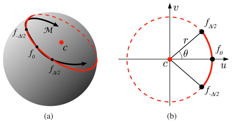
Although the Taylor series provides the most intuitive and well-known method of approximating time-shifts, we have developed an alternative interpolator that is much more accurate. The solution is motivated by the observation that the manifold of time-shifted waveforms, f_τ(t), must lie on the surface of a hypersphere (because the waveform L₂-norm is preserved under translation), and furthermore, must have a constant curvature (by symmetry). This leads to the notion that it might be well-approximated by an arc of a circle. As such, we approximate a segment of the manifold, { $f_{\tau }:\mid \tau \mid \le \frac{\mathrm{\Delta }}{2}$}, by the unique circular arc that contains the three points {f_−Δ/2, f₀, f_Δ/2}, as illustrated in Fig. 3(a). The resulting interpolator is an example of a trigonometric spline [27], in which the three time-shifted functions are linearly combined using trigonometric coefficients to approximate intermediate translates of f(t):

$$f_{\tau }(t)\approx c(t)+rcos(\frac{2\tau }{\mathrm{\Delta }}\theta )u(t)+rsin(\frac{2\tau }{\mathrm{\Delta }}\theta )v(t)$$ (14)

Fig. 3.

Illustration of the polar interpolator. (a) The manifold of time shifts of f(t) (black line) lies on the surface of a hypersphere. We approximate a segment of this manifold, for time shifts $\tau \in [-\frac{\mathrm{\Delta }}{2},\frac{\mathrm{\Delta }}{2}]$, with a portion of a circle (red), with center defined by c(t). (b) Parameterization of the circular arc approximation.

The functions {c(t), u(t), v(t)} are computed from linear combinations of {f_−Δ/2, f₀, f_Δ/2}:

$$\left(\begin{array}{c}{f}_{-\frac{\mathrm{\Delta }}{2}}(t)\\ f_0(t)\\ f_{\frac{\mathrm{\Delta }}{2}}(t)\end{array}\right)=\left(\begin{array}{ccc}1& rcos(\theta )& -rsin(\theta )\\ 1& r& 0\\ 1& rcos(\theta )& rsin(\theta )\end{array}\right)\left(\begin{array}{c}c(t)\\ u(t)\\ v(t)\end{array}\right)$$ (15)

The constants r and θ are the radius and half the subtended angle of the arc, respectively, both of which depend on f(t) and can be computed in closed form. These relationships are illustrated in Fig. 3(b). Combining Eq. (14–15) gives:

$$f_{\tau }(t)={\left(\begin{array}{c}1\\ rcos(\frac{2\tau }{\mathrm{\Delta }}\theta )\\ rsin(\frac{2\tau }{\mathrm{\Delta }}\theta )\end{array}\right)}^T{A}^{-1}\left(\begin{array}{c}{f}_{-\frac{\mathrm{\Delta }}{2}}(t)\\ f_0(t)\\ f_{\frac{\mathrm{\Delta }}{2}}(t)\end{array}\right)$$ (16)

where A is the matrix in Eq. (15). The approximation can be more clearly understood in the frequency domain by taking the Fourier transform and dividing both sides by f̂(ω):

$$e^{-i\omega \tau }\approx (1-2a(\tau ))+e^{i\omega \frac{\mathrm{\Delta }}{2}}(a(\tau )-b(\tau ))+e^{-i\omega \frac{\mathrm{\Delta }}{2}}(a(\tau )+b(\tau ))$$ (17)

where

$$a(\tau )=\frac{cos(\frac{2\tau \theta }{\mathrm{\Delta }})-1}{2(cos(\theta )-1)}\text{and}b(\tau )=\frac{sin(\frac{2\tau \theta }{\mathrm{\Delta }})}{2sin(\theta )}.$$

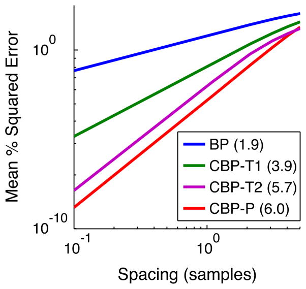
Figure 4 compares nearest neighbor (implicitly used in BP), first-order Taylor, and polar interpolation in terms of their accuracy in approximating time-shifts of a Gaussian derivative waveform, f(t) ∝ te^−αt₂. For reference, the second-order Taylor interpolator is also included. The polar interpolator is seen to be much more accurate than nearest-neighbor and 1st-order Taylor, and even surpasses 2nd-order Taylor by an order of magnitude (although they have the same asymptotic rate of convergence). This allows one to choose a much larger Δ for a given desired accuracy.

Fig. 4.

Comparison of the nearest neighbor, first-order Taylor, and polar interpolators (as used in BP, CBP-T, and CBP-P, respectively) for a waveform f(t) ∝ te^−αt2. Second-order Taylor interpolation are also shown. The estimated log-domain slopes (asymptotic rates of convergence) are indicated in parenthesis in the legend.

We now construct a dictionary of time-shifted copies of the functions used to represent the polar interpolation, {c_iΔ, u_iΔ, v_iΔ}, and form a convex set from these to approximate the manifold:

$${\mathcal{M}}_{f,T}\approx \left\{{xc}_{i\mathrm{\Delta }}(t)+{yu}_{i\mathrm{\Delta }}(t)+{zv}_{i\mathrm{\Delta }}(t):\begin{array}{l}x\ge 0,\hfill \\ y^2+z^2\le x^2{r}^2,\hfill \\ \mathit{xr}cos(\theta )\le y\le xr,\hfill \\ i=1,\dots N_{\mathrm{\Delta }}\hfill \end{array}\right\}$$ (18)

The constraints on the coefficients (x, y, z) ensure that they represent a scaled translate of f(t), except for the second, which is a convex relaxation of the true constraint, y² + z² = x²r² (see below). As with the Taylor approximation, we have a one-to-one correspondence between event amplitudes/time-shifts and the constrained coefficients:

$$\sum _i{x}_i{c}_{i\mathrm{\Delta }}(t)+y_i{u}_{i\mathrm{\Delta }}(t)+z_i{v}_{i\mathrm{\Delta }}(t)\approx \sum _i{x}_i{f}_{(i\mathrm{\Delta }-\frac{\mathrm{\Delta }}{2\theta }{tan}^{-1}(z_i/y_i))}(t)$$ (19)

as long as z_i/y_i ≠ tan(θ) for all i. The inference problem again boils down to minimizing a constrained convex objective function:

$$\begin{array}{l}\underset{\overrightarrow{x},\overrightarrow{y},\overrightarrow{z}}{min}\frac{1}{2{\sigma }^2}{\Vert y(t)-(C_{\mathrm{\Delta }}\overrightarrow{x})(t)-(U_{\mathrm{\Delta }}\overrightarrow{y})(t)-(V_{\mathrm{\Delta }}\overrightarrow{z})(t)\Vert }_2^2+\lambda {\Vert \overrightarrow{x}\Vert }_1\\ \text{s}.\text{t}.\left\{\begin{array}{l}{x}_i\ge 0,\hfill \\ \sqrt{y_i^2+z_i^2}\le x_{i}r,\hfill \\ x_{i}rcos(\theta )\le y_i\le x_{i}r,\hfill \end{array}\right\}\text{for}i=1,\dots N_{\mathrm{\Delta }}\end{array}$$ (20)

where C_Δ, U_Δ, V_Δ are dictionaries containing Δ-shifted copies of c(t), u(t), v(t), respectively. Equation (20) is an example of a “second-order cone program” for which efficient solvers exist ([28]). After the optimum values for {x⃗, y⃗, z⃗} are obtained, time-shifts and amplitudes can be inferred by first projecting the solution back to the original constraint set:

$$(x_i,y_i,z_i)\leftarrow (x_i,\frac{y_i{x}_{i}r}{\sqrt{y_i^2+z_i^2}},\frac{z_i{x}_{i}r}{\sqrt{y_i^2+z_i^2}})$$ (21)

and then using Eq. (19) to solve for the event times.

Figure 2(c) illustrates the optimization of Eq. (20) for the simple example described in the previous section. Notice that the solution corresponding to λ = 0 (yellow dot) is substantially sparser relative to both the CBP-T and BP solutions, and that the solution becomes L₀ sparse if λ is increased by just a small amount, giving up very little reconstruction accuracy.

C. General interpolation

We can generalize the CBP approach to use any linear interpolation scheme. Suppose we have a set of basis functions ${\{{\phi }_n(t)\}}_1^m$ in L₂([0, T]) and a corresponding interpolation map $D:[-\frac{\mathrm{\Delta }}{2},\frac{\mathrm{\Delta }}{2}]\to {\mathbb{R}}^m$ such that local shifts can be approximated as:

$$f_{\tau }(t)\approx \sum _{n=1}^m{D}_n(\tau ){\phi }_n(t),\mid \tau \mid \le \frac{\mathrm{\Delta }}{2}.$$ (22)

(e.g., Eq. (9) and Eq. (14)). Let S be the set of all nonnegative scalings of the image of [ $-\frac{\mathrm{\Delta }}{2},\frac{\mathrm{\Delta }}{2}$] under the interpolator:

$$S=\{a\overrightarrow{x}:a\ge 0,\overrightarrow{x}\in \text{Range}(D)\}.$$

In general, S may not be convex (as in the polar case), and we denote its convex hull by . If we have a set of coefficients x⃗ ∈ ℝ^N_Δ×m where each block x⃗_i := [x_i1, …, x_im] is in , then the signal given by:

$$\sum _{i=1}^{N_{\mathrm{\Delta }}}\sum _{n=1}^m{x}_{in}{\phi }_n(t-i\mathrm{\Delta })$$ (23)

approximates a sum of scaled and translated waveforms. If D is invertible, the amplitudes and shifts are obtained as follows:

$$a_i\leftarrow a\text{s}.\text{t}.\frac{P_S({\overrightarrow{x}}_i)}{a}\in \text{Range}(D)$$ (24)

$${\tau }_i\leftarrow i\mathrm{\Delta }+D^{-1}(P_S({\overrightarrow{x}}_i)/a)$$ (25)

where P_S(.) projects points in onto S. Note that in this general form, the L₂ norm of (the projection of) each group x⃗_i governs the amplitude of the corresponding time-shifted waveform.³ Finally, we can obtain the coefficients by solving:

$$\underset{\overrightarrow{x}}{min}\frac{1}{2{\sigma }^2}{\Vert y(t)-({\mathrm{\Phi }}_{\mathrm{\Delta }}\overrightarrow{x})\Vert }_2^2+\lambda \sum _{i=1}^{N_{\mathrm{\Delta }}}{\Vert {\overrightarrow{x}}_i\Vert }_2\text{s}.\text{t}.{\overrightarrow{x}}_i\in \mathcal{H}\text{for}i=1,\dots ,N_{\mathrm{\Delta }}$$ (26)

where the linear operator Φ_Δ is defined as:

$$({\mathrm{\Phi }}_{\mathrm{\Delta }}\overrightarrow{x})(t):=\sum _{i=1}^{N_{\mathrm{\Delta }}}\sum _{n=1}^m{x}_{in}{\phi }_n(t-i\mathrm{\Delta })$$

Equation (26) can be solved efficiently using standard convex optimization methods (e.g., interior point methods [28]). It is similar to the objective functions used to recover so-called “block-sparse” signals (e.g., [12], [29]), but includes auxiliary constraints on the coefficients to ensure that only signals close to span( ) are represented. Table I summarizes the Taylor and polar interpolation examples within this general framework, along with the case of nearest-neighbor interpolation (which corresponds to standard BP).

TABLE I.

Property	BP (nearest neighbor)	CBP - Taylor interp	CBP - polar interp
basis: ${\{{\phi }_n(t)\}}_{n=1}^m$	[f(t)]	[f(t), f′(t)]	[c(t), u(t), v(t)]
interpolator: D⃗(τ)	1	[1, τ]T	${[1,rcos(\theta \frac{2\tau }{\mathrm{\Delta }}),rsin(\theta \frac{2\tau }{\mathrm{\Delta }})]}^T$
constrained coefficient set: S	{x1 ≥ 0}	{x1 ≥ 0, $\mid x_2\mid \le x_1\frac{\mathrm{\Delta }}{2}$}	{x1 ≥ 0, $x_2^2+x_3^2=r^2{x}_1^2$, rx1 cos(θ) ≤ x2 ≤ rx1}
convex relaxation:	S	S	{x1 ≥ 0, $x_2^2+x_3^2\le r^2{x}_1^2$, rx1 cos(θ) ≤ x2 ≤ rx1}
projection operator: PS(x⃗)	x⃗	x⃗	${[x_1,r{x}_1\frac{x_2}{\sqrt{x_2^2+x_3^2}},r{x}_1\frac{x_3}{\sqrt{x_2^2+x_3^2}}]}^T$

The quality of the solution relies on the accuracy of the interpolator, the convex approximation ≈ S, and the ability of the block-L₁ based penalty term in Eq. (26) to achieve L₀-sparse solutions that reconstruct the signal accurately. The first two of these are relatively straightforward, since they depend solely on the properties of the interpolator (see Fig. 4). The last is difficult to predict, even for the simple examples illustrated in Figure 2. The level sets of the L₂ term can have a complicated form when taking the constraints into account, and it is not clear a priori whether this will facilitate or hinder the L₁ term in achieving sparse solutions. Nevertheless, our empirical results clearly indicate that solving Eq. (26) with Taylor and polar interpolators yields substantially sparser solutions than those achieved with standard BP.

V. Empirical results

We evaluate our method on data simulated according to the generative model of Eq. (2). Event amplitudes were drawn uniformly from the interval [0.5, 1.5]. We used a single template waveform f(t) ∝ te^−αt2 (normalized, so that ||f||₂ = 1), for which the interpolator performances are plotted in Fig. 4. We compared solutions of Eqs. (7), (13), and (20). Amplitudes were constrained to be nonnegative (this is already assumed for the CBP methods, and amounts to an additional linear inequality constraint for BP). Each method has two free parameters: Δ controls the spacing of the basis, and λ controls the tradeoff between reconstruction error and sparsity. We varied these parameters systematically and measured performance in terms of two quantities: (1) signal reconstruction error (which decreases as λ or Δ decreases), and (2) sparsity of the estimated event amplitudes, which increases as λ increases. The former is simply the first term in the objective function (for all three methods). For the latter, to ensure numerical stability, we used the L_p norm with p = 0.1 (results were stable with respect to the choice of p, as long as p < 1 and p was not below the numerical precision of the optimizations). Computations were performed numerically, by sampling the functions f(t) and y(t) at a fine constant spacing. We used the convex solver package CVX [30] to obtain numerical solutions.

A small temporal window of the events recovered by the three methods is provided in Fig. 5. The three plots show the estimated event times and amplitudes for BP, CBP-T, and CBP-P (upward stems) compared to the true event times/amplitudes (downward stems). The figure demonstrates that CBP, equipped with either Taylor or polar interpolators, is able to recover the event train more accurately, and with a larger spacing between basis functions (indicated by the tick marks on the x-axis). As predicted by the reasoning laid out in Figure 2(a), basis pursuit tends to split events across two or more adjacent low-amplitude coefficients, thus producing less sparse solutions and making it hard to infer the number of events and their respective amplitudes and times. Sparsity can be improved by increasing λ, but at the expense of a substantial increase in approximation error.

Fig. 5.

Sparse signal recovery using BP (Eq. (7)), CBP-T (Eq. (13)), and CBP-P (Eq. (20)). The source was a sparse superposition of arbitrarily time-shifted copies of the function f(t) ∝ te^−αt2. The SNR (defined as ||f||_∞/σ) was 12 with identical signal and noise for all three examples. For each method, the values of Δ and λ were chosen to minimize the sum of squares of sparsity and reconstruction error (large dots in Fig. 6). Upward stems indicate the estimated magnitudes, placed at locations determined by the interpolation coefficients via Eq. (24). Amplitudes less than 0.01 were eliminated for clarity. Ticks denote the location of the basis functions corresponding to each upward-pointing stem. Downward stems indicate true locations and magnitudes.

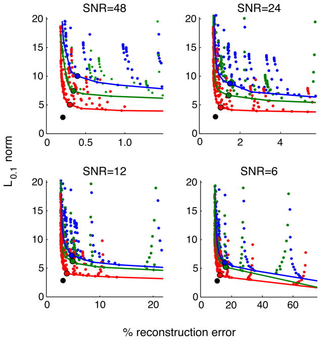
Figure 6 illustrates the tradeoff between sparsity and approximation error for each of the methods. Each panel corresponds to a different noise level. The individual points, color-coded for each method, are obtained by running the associated method 500 times for a given (Δ, λ) combination, and averaging the errors over these trials. The solid curves are the (numerically computed) convex hulls of all points obtained for each method, and clearly indicate the tradeoff between the two types of error. We can see that the performance of BP is strictly dominated by that of CBP-T: For every BP solution, there is a CBP-T solution that has lower values for both error types. Similarly, CBP-T is strictly dominated by CBP-P, which can be seen to come close to the error values of the ground truth answer (which is indicated by a black dot). Note that the reconstruction error of the true solution and of all methods is bounded below by the variance of the noise that lies outside of the subspace spanned by the set of shifted copies of the waveform.

Fig. 6.

Error plots for 4 noise levels (SNR is defined as ||f||_∞/σ)). Each graph shows the tradeoff between the average reconstruction error and sparsity (measured as average L_0.1 norm of estimated amplitudes). Each point represents the error values for one of the methods, applied with a particular setting of (Δ, λ), averaged over 500 trials. Colors indicate the method used (blue:BP, green:CBP-T, red:CBP-P). Bold lines denote the convex hulls of all points for each method. The large dots indicate the “best” solution, as measured by Euclidean distance from the correct solution (indicated by black dots).

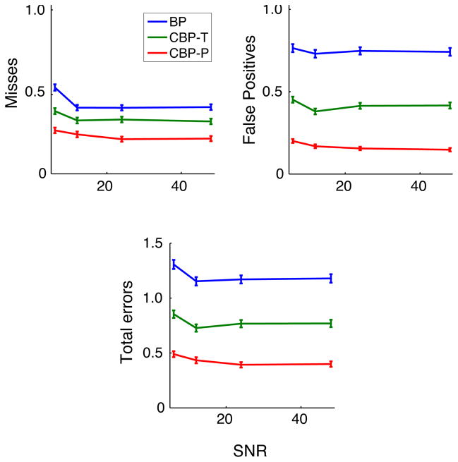
We performed a signal detection analysis of the performance of these methods, classifying identification errors as misses and false positives. We match an estimated event with a true event if the estimated location is within 3 samples of the true event time, the estimated amplitude is within a threshold $\frac{1}{\sqrt{12}}$ of the true amplitude (one standard deviation of the amplitude distribution Unif ([0.5, 1.5])), and no other estimated event has been matched to the true event. We found that results were relatively stable with respect to the threshold choices. For each method and noise level we chose the (λ, Δ) combination yielding a solution closest to ground truth (corresponding to the large dots in Figure 6). Figure 7 shows the errors as a function of the noise level. We see that performance of all methods is surprisingly stable across SNR levels. We also see that BP performance is dominated at all noise levels by CBP-T, which has fewer misses as well as fewer false positives, and CBP-T is similarly dominated by CBP-P.

Fig. 7.

Signal detection analysis of solutions at three SNR levels. (see text). Misses, false positives, and total errors (sum of misses and false positives), as a fraction of the mean number of events, were computed over 500 trials for each method, and for each SNR (defined as |f||_∞/σ)).

Finally, Fig. 8 shows the distribution of the amplitudes estimated by each algorithm, and compare with the distribution of the source, as given by Eq. (4). We see that CBP-P produces amplitude distributions that are far better-matched to the correct distribution of amplitudes.

Fig. 8.

Histograms of the estimated amplitudes for BP, CBP-T, and CBP-P, respectively. All methods were constrained to estimate only nonnegative amplitudes, but no upper bound was imposed. The true distribution of amplitudes is given by Eq. (4), and is indicated in red.

A. Multiple features

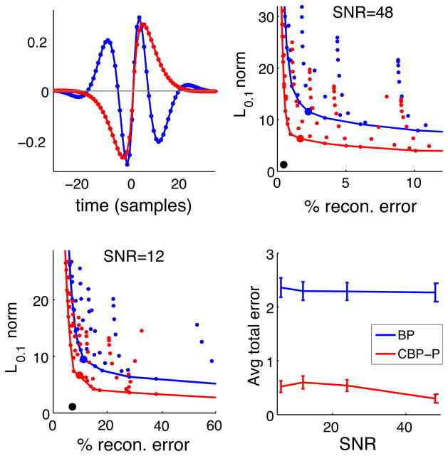
All the methods we described can be extended to the case of multiple templates by taking as a dictionary the union of dictionaries associated with each individual template. We performed a final set of experiments using two “gammatone” features (shown in upper left of Fig. 9), which are commonly used in audio processing. Event times were sampled from two correlated Poisson processes with the same marginal rate λ₀ and a correlation of ρ = 0.5. These were generated by independently sampling 2 Poisson process with rate λ₀(1 − ρ) and then superimposing a randomly jittered “common” Poisson process with rate λ₀ρ. As before, event amplitudes were drawn uniformly from the interval [0.5, 1.5]. We compared the performance of BP and CBP-P, in both cases using dictionaries formed from the union of dictionaries for each template with a common spacing, Δ, for both templates. In general, the spacing could be chosen differently for each waveform, providing more flexibility at the expense of additional parameters that must be calibrated. The upper right and lower left plots in Fig. 9 show the error tradeoff for different settings of (Δ, λ) at SNR levels of 48 and 12, respectively (the results were qualitatively unchanged for SNR values of 24 and 6). The lower right plot in Fig. 9 plots the total number of event identification errors (misses plus false positives) for each method as a function of SNR, at each method’s optimal (Δ,λ) setting.

Fig. 9.

Sparse signal decomposition with two wavefoms. Upper-left: Gammatone waveforms, f_i(t) = atⁿ⁻¹e^−2πbt cos(2πω_it) for i = 1, 2. Upper-right and lowe-left: Sparsity and reconstruction errors for BP (blue) and CBP-P (red), as in Figure 6, with SNR’s of 48 and 12, respectively (again, SNR is defined as ||f||_∞/σ)). Lower right: total number of misses and false positives (with same thresholds as in bottom plot of Figure 7) for each method.

VI. Discussion

We have introduced a novel methodology for sparse signal decomposition in terms of continuously shifted features. The method can be seen as a continuous form of the well-known basis pursuit method, and we thus have dubbed it continuous basis pursuit. The method overcomes the limitation of basis pursuit in the convolutional setting caused by the tradeoff between discretization error and the effectiveness of the L₁ relaxation for obtaining sparse solutions. In particular, our method employs an alternative discrete basis (not necessarily the features themselves) which can explicitly account for the continuous time-shifts present in the signal. We derived a general convex objective function that can be used with any such basis. The coefficients are constrained so as to represent only transformed versions of the templates, and the objective function uses an L₁ norm to penalize the amplitudes of these transformed versions . We showed empirically that using simple first-order (Taylor) and second-order (polar) interpolation schemes yields superior solutions in the sense that (1) they are sparser, with improved reconstruction accuracy, (2) they produce substantially better identification of events (fewer misses and false positives), and (3) the amplitude statistics are a better match to those of the true generative model. We showed that these results are stable across a wide range of noise levels. We conclude that an interpolating basis, coupled with appropriate constraints on coefficients, provides a powerful and tractable tool for modeling and decomposing sparse translation-invariant signals.

We believe our method can be extended for use with other types of signal, as well as to transformations other than translation. For example, for one-dimensional signals such as audio, one might also include dilation or frequency-modulation of the templates. Both the Taylor and polar basis constructions can be extended to account for multiple transformations. In the Taylor case, one only needs to add incorporate waveform derivatives with respect to each transformation (with a separate constraint for each of their coefficients). In the polar case, one can model the manifold of local (renormalized) translations and dilations as a 2D patch on the surface of a sphere, ellipsoid, or torus (instead of a 1D arc) which can be parameterized with two angles. For images, one could include rotation along with dilation (e.g., [31]). In general, the primary hurdles for such extensions are to specify (1) the form of the linear interpolation (for joint variables, this might be done separably, or using a multi-dimensional interpolator), (2) the constraints on coefficients (and a convex relaxation of these costraints), and (3) a means of inverting the interpolator so as to obtain transformation parameters from recovered coefficients. Another natural extension is to use CBP in the context of learning optimal features for decomposing an ensemble of signals, as has been previously done with BP (e.g., [8], [10], [4], [11], [32]).

Although we have described the use of an interpolator basis in the context of L₁-based recovery methods, we believe the same representations can be used to improve other recovery methods (e.g., greedy or iterative thresholding methods with a convolutional basis). Furthermore, our polar approximation of a translational manifold can provide a substrate for new forms of sampling (e.g., [33], [34], [35]). By introducing a basis and constraints that explicitly model the local geometry of the manifold on which the signals lie, we expect our method to offer substantial improvements in many of the applications for which sparse signal decomposition has been found useful.

Biographies

Chaitanya Ekanadham received his B.S. in mathematical/computational sciences and symbolic systems from Stanford University in 2007. He is currently a Ph.D. candidate in applied math at the Courant Institute, New York University, working with Eero Simoncelli and Daniel Tranchina. His research interests lie at the intersection of statistical signal processing, machine learning, and applied mathematics.

Daniel Tranchina Daniel Tranchina received his Ph.D. from The Rockefeller University in 1981, and his B.A. in Chemistry from The State University of New York at Binghamton in 1975. His graduate training and postdoctoral studies were in mathematics and experimental neuroscience. In 1984 he became a faculty member at New York University, where he is currently a Professor of Biology, Mathematics and Neural Science. His research interests include computational neuroscience, phototransduction, neural network modeling, population density methods, stochastic gene expression, and statistical analysis and modeling of genomic data.

Eero P. Simoncelli received the BS degree (summa cum laude) in physics from Harvard University in 1984 and the MS and PhD degrees in electrical engineering from Massachusetts Institute of Technology in 1988 and 1993, respectively. He studied applied mathematics at Cambridge University for a year and a half. He was an assistant professor in the Computer and Information Science Department at the University of Pennsylvania from 1993 to 1996. In September 1996, he moved to New York University, where he is currently an associate professor in neural science and mathematics. In August 2000, he became an associate investigator at the Howard Hughes Medical Institute under their new program in computational biology. His research interests span a wide range of topics in the representation and analysis of visual images, in both machine and biological systems. He is a fellow of the IEEE.

References

- 1.Rothwell EJ, Sun W. Time domain deconvolution of transient radar data. Antennas and Propagation, IEEE Transactions on. 1990 Apr;38(4):470–475. [Google Scholar]
- 2.Mendel J. Optimal Seismic Deconvolution: An Estimation Based Approach. Academic Press; 1983. [Google Scholar]
- 3.Patterson RD, Robinson K, Holdsworth J, McKeown D, Zhan C, Allerhand M. Complex sounds and auditory images. Auditory physiology and perception, Proceedings of the 9th International Symposium on Hearing; 1992. pp. 429–446. [Google Scholar]
- 4.Smith Evan, Lewicki Michael S. Efficient coding of time-relative structure using spikes. Neural Computation. 2005 Jan;17(1):19–45. doi: 10.1162/0899766052530839. [DOI] [PubMed] [Google Scholar]
- 5.Grosse Roger, Raina Rajat, Kwong Helen, Ng Andrew Y. UAI. 2007. Shift-invariant sparse coding for audio classification. [Google Scholar]
- 6.Simoncelli EP, Freeman WT. The steerable pyramid: A flexible architecture for multi-scale derivative computation. Proc 2nd IEEE Int’l Conf on Image Proc; Washington, DC. Oct 23–26 1995; IEEE Sig Proc Society; pp. 444–447. [Google Scholar]
- 7.Mallat Stephane. A wavelet tour of signal processing. Academic Press; 1999. [Google Scholar]
- 8.Sallee Phil, Olshausen Bruno A. Learning sparse multiscale image representations. NIPS. 2002:1327–1334. [Google Scholar]
- 9.Candès EJ, Demanet L, Donoho DL, Ying L. Fast discrete curvelet transforms. Multiscale Modeling and Simulation. 2005;5 [Google Scholar]
- 10.Olshausen BA, Field DJ. Emergence of simple-cell receptive field properties by learning a sparse code for natural images. Nature. 1996 Jun;381(6583):607–609. doi: 10.1038/381607a0. [DOI] [PubMed] [Google Scholar]
- 11.Bell AJ, Sejnowski TJ. The “independent components” of natural scenes are edge filters. Vision Res. 1997 Dec;37(23):3327–3338. doi: 10.1016/s0042-6989(97)00121-1. [DOI] [PMC free article] [PubMed] [Google Scholar]
- 12.Hyvärinen A, Hoyer P. Emergence of phase- and shift-invariant features by decomposition of natural images into independent feature subspaces. Neural Computation. 2000 Jul;12(7):1705–1720. doi: 10.1162/089976600300015312. [DOI] [PubMed] [Google Scholar]
- 13.Friedman JH, Tukey JW. A projection pursuit algorithm for exploratory data analysis. IEEE Trans Computers. 1974;C-23(9):881–890. [Google Scholar]
- 14.Mallat Stephane, Zhang Zhifeng. Matching pursuits with time-frequency dictionaries. IEEE Trans Sig Proc. 1993 Dec;41(12):3397–3415. [Google Scholar]
- 15.Tropp JA. Greed is good: Algorithmic results for sparse approximation. IEEE Trans Inform Theory. 2004;50(10):2231–2242. [Google Scholar]
- 16.Blumensath T, Davies ME. Iterative thresholding for sparse approximations. J Fourier Analysis and Applications. 2004 [Google Scholar]
- 17.Elad M. Why simple shrinkage is still relevant for redundant representations. IEEE Trans Info Theory. 2006;52:5559–5569. [Google Scholar]
- 18.Bioucas-Dias J, Figueiredo M. A new TwIST: Two-step iterative shrinkage/thresholding algorithms for image restoration. IEEE Trans Image Processing. 2007;16(12):2992–3004. doi: 10.1109/tip.2007.909319. [DOI] [PubMed] [Google Scholar]
- 19.Figueiredo MAT, Bioucas-Dias JM, Nowak RD. Majorization–minimization algorithms for wavelet-based image restoration. Image Processing, IEEE Transactions on. 2007;16(12):2980–2991. doi: 10.1109/tip.2007.909318. [DOI] [PubMed] [Google Scholar]
- 20.Tibshirani Robert. Regression shrinkage and selection via the lasso. Journal of the Royal Statistical Society Series B (Methodological) 1996;58(1):267–288. [Google Scholar]
- 21.Chen Scott Shaobing, Donoho David L, Saunders Michael A. Atomic decomposition by basis pursuit. SIAM Journal on Scientific Computing. 1998;20(1):33–61. [Google Scholar]
- 22.Ekanadham C, Tranchina D, Simoncelli EP. Sparse decomposition of transformation-invariant signals with continuous basis pursuit. Proc. IEEE Int Acoustics, Speech and Signal Processing Conf. ICASSP 2011; 2011. [DOI] [PMC free article] [PubMed] [Google Scholar]
- 23.Davis G, Mallat S, Avellaneda M. Adaptive greedy approximations. Constructive Approximation. 1997;13:57–98. doi: 10.1007/BF02678430. [DOI] [Google Scholar]
- 24.Taylor HL, Banks SC, McCoy JF. Deconvolution with the 11 norm. Geophysics. 1979;44(1):39. [Google Scholar]
- 25.O’Brien MS, Sinclair AN, Kramer SM. Recovery of a sparse spike time series by 11 norm deconvolution. Signal Processing, IEEE Transactions on. 1994 Dec;42(12):3353–3365. [Google Scholar]
- 26.Candès EJ, Romberg J, Tao T. Robust uncertainty principles: exact signal reconstruction from highly incomplete frequency information. IEEE Trans IT. 2006;52(2):489–509. [Google Scholar]
- 27.Schoenberg IJ. On trigonometric spline interpolation. Journal of Math Mech. 1964;13:795–825. [Google Scholar]
- 28.Boyd Stephen, Vandenberghe Lieven. Convex Optimization. Cambridge University Press; 2004. [Google Scholar]
- 29.Eldar YC, Mishali M. Robust recovery of signals from a structured union of subspaces. IEEE Transactions on Information Theory. 2009;55(11):5302–5316. [Google Scholar]
- 30.Grant M, Boyd S. CVX: Matlab software for disciplined convex programming, version 1.21. 2010 Oct; http://cvxr.com/cvx.
- 31.Manifold models for signals and images. Computer vision and image understanding. 2009;113(2):249–260. [Google Scholar]
- 32.Berkes P, Turner RE, Sahani M. A structured model of video reproduces primary visual cortical organisation. PLoS Computational Biology. 2009;5(9) doi: 10.1371/journal.pcbi.1000495. [DOI] [PMC free article] [PubMed] [Google Scholar]
- 33.Unser M. Sampling-50 years after shannon. Proceedings of the IEEE. 2000;88(4):569–587. [Google Scholar]
- 34.Vetterli M, Marziliano P, Blu T. Sampling signals with finite rate of innovation. IEEE Trans Sig Proc. 2002 Jun;50(6):1417–1428. [Google Scholar]
- 35.Uriguen J, Eldar YC, Dragotti PL, Ben-Haim Z. Sampling at the Rate of Innovation: Theory and Applications. Cambridge University Press; 2011. [Google Scholar]