Large-scale cortical correlation structure of spontaneous oscillatory activity

Abstract

Little is known about the brain-wide correlation of electrophysiological signals. Here we show that spontaneous oscillatory neuronal activity exhibits frequency-specific spatial correlation structure in the human brain. We developed an analysis approach that discounts spurious correlation of signal power caused by the limited spatial resolution of electrophysiological measures. We applied this approach to source estimates of spontaneous neuronal activity reconstructed from magnetoencephalography (MEG). Overall, correlation of power across cortical regions was strongest in the alpha to beta frequency range (8–32 Hz) and correlation patterns depended on the underlying oscillation frequency. Global hubs resided in the medial temporal lobe in the theta frequency range (4–6 Hz), in lateral parietal areas in the alpha to beta frequency range (8–23 Hz), and in sensorimotor areas for higher frequencies (32–45 Hz). Our data suggest that interactions in various large-scale cortical networks may be reflected in frequency specific power-envelope correlations.

Introduction

As a measure of functional connectivity, the co-variation of spontaneous hemodynamic signals has revealed fundamental insights into the large-scale functional organization of the human brain^1,2. Blood oxygen level-dependent functional magnetic resonance imaging (BOLD fMRI) has provided consistent evidence for correlated fluctuations of spontaneous neuronal activity within highly structured networks of brain regions^3–9. The gross spatial correlation structure that constitutes these networks is highly robust and often studied during resting fixation. Furthermore, the correlation structure also reflects task demands^8,10, the subjects’ conscious state¹¹, as well as psychiatric and neurological disorders^12,13.

However, an important limitation of the available fMRI studies is that hemodynamic signals provide merely an indirect measure of neuronal activity^14–16. In contrast, electroencephalography (EEG) and magnetoencephalography (MEG) directly measure the electrophysiological activity of interest. Furthermore, with their high temporal resolution, these electrophysiological measures sample the rich temporal dynamics of neuronal population activity. These temporal dynamics entail neuronal oscillations that, with their specific frequencies, reflect the biophysical properties of different local and large-scale network interactions^17–19. Thus, connectivity measures based on specific spectral components of neuronal population activity may provide qualitatively new insights into the circuit mechanisms underlying the large-scale organization of brain activity¹⁹. However, currently little is known about the brain-wide correlation of such frequency-specific neuronal population signals. To characterize the brain-wide correlation structure of oscillatory power, we developed a new analysis approach that overcomes current methodological limitations in EEG and MEG for investigating large-scale functional connectivity. We applied this approach to MEG recordings of healthy human subjects during resting fixation.

Results

We recorded MEG from 43 subjects that were instructed to fixate a centrally presented cross (average duration: ~500 s). We applied time-frequency transformation and linear ‘beamforming’ to the MEG data to derive temporally, spectrally, and spatially resolved estimates of neuronal population activity. The temporal evolution of spectral power (power envelope) in different brain regions around a given carrier frequency served as the signal for our correlation analysis²⁰ (Fig. 1a). Notably, the correlation between power envelopes investigated here should not be confused with measures of the phase relation between the underlying signals, such as e.g. coherence^19,21–23.

Figure 1.

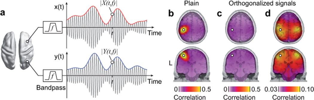
Power envelope correlation. (a) Illustration of spectrally resolved power envelopes for one exemplary carrier frequency f (i.e. center frequency of the band-pass filter). The gray sinusoidal lines represent band-pass filtered neuronal signals estimated at two source locations. The corresponding blue and red lines – the amplitude envelopes – quantify the evolution of the signal amplitude at a slower time-scale. We used the logarithm of the squared amplitude envelopes (power envelopes) for correlation analyses. (b) Plain power envelope correlation between the left somatosensory cortex (white circle) and the rest of the brain at a carrier frequency of 16 Hz. The correlation values are overlaid on cortical slices intersecting the seed location. (c) Power envelope correlation between orthogonalized signals from the left somatosensory cortex (white circle) and the rest of the brain at a carrier frequency of 16 Hz. Note, the color scale is identical to b. (d) Same as in c but scaled to the minimal and maximal correlation value occurring.

It is difficult to investigate the relation between neuronal population signals from EEG and MEG because of profound methodological problems^19,23–25. Due to the limited spatial resolution of EEG and MEG, even distant sensors or source estimates are sensitive to the same neuronal sources. In source space, this translates into a trivial spatial interaction pattern that drops off with distance from any reference location. Figure 1b illustrates this problem for the power envelope correlation between a reference location in the left somatosensory cortex and the rest of the brain. The spatial correlation pattern is dominated by an unstructured decay from the reference site that is caused by the fact that source estimates close to the reference location are sensitive to the same true sources as the reference estimate. This spurious correlation pattern is problematic since it masks the physiological correlation structures of interest. To overcome this problem, we developed a new analysis approach for studying functional connectivity based on power envelope correlations.

Power envelope correlation between orthogonalized signals

Electrical and magnetic neuronal signals are measured virtually instantaneously at different sensors. Thus, signal components that reflect the same source at two different sensors (or source estimates) are characterized by an identical phase²⁴. In contrast, for many cases, signals from different neuronal populations can be thought of as having a variable phase relation. We exploited this difference to discount the spurious correlation pattern caused by the limited spatial resolution of MEG. For each pair of signals, time window, and carrier frequency, we removed the signal components that shared the same phase before computing the signals’ power estimates. In other words, we orthogonalized the signals before deriving their power envelopes. As a measure of interaction we then computed the linear correlation between these power envelopes. This procedure ensures that the signals do not share the trivial correlation in power due to the methodological problems described above (see Online Methods, Supplementary Data, and Supplementary Figs. 1 and 2 for details). Applying this approach to the above example had a strong effect. The pattern that dominated the plain correlation vanished, which revealed residual correlation of much smaller magnitude (Fig. 1c). This residual spatial correlation pattern (Fig. 1d, note the different color scale as compared to Fig. 1c) was highly structured and extended to distant cortical areas. Correlation was strongest to the vicinity of the reference and to the homologous somatosensory cortex in the other hemisphere.

We next derived the correlation between all 2,925 locations on a regular 3D grid covering the entire brain. The average correlation was significantly higher than zero for all carrier frequencies from 2 to 128 Hz (t-test, P < 0.05, false discovery rate (FDR) corrected). Average correlation was strongest in the alpha to beta frequency range (r: 0.069 ± 0.060, mean ± s.d. at 16 Hz) with about 90% of positive correlations. To identify spatial structure within the correlation, we statistically tested for correlation higher than the average correlation across the brain. As a starting point, we followed up on the introductory example and analyzed interhemispheric correlation between homologous early sensory areas across different modalities.

Inter-hemispheric correlation between homologous sensory areas

A fundamental property of human brain anatomy is that most homologous areas in the two hemispheres are anatomically connected. Accordingly, fMRI studies^1,26, intracranial recordings²⁷, and MEG studies^28,29 have found that homologous sensory areas exhibit correlated spontaneous activity. Consequently, we expected to find a related pattern for power-envelope correlations using our new analysis approach.

We focused on bilateral early auditory, visual, and somatosensory cortices and investigated a broad range of different carrier frequencies (Fig. 2a). In all three sensory systems, we found the strongest correlation in the alpha to beta carrier-frequency range (8–32 Hz). The analysis of the brain-wide correlation at 16 Hz – the center of this frequency range – revealed that the correlation between homologous sensory cortices was spatially specific (Fig. 2b–d; one-sided t-test for correlation > average correlation, P < 0.05, FDR corrected). The strongest correlations were expressed to areas in direct proximity to the reference locations and to the homologous cortex in the contralateral hemisphere.

Figure 2.

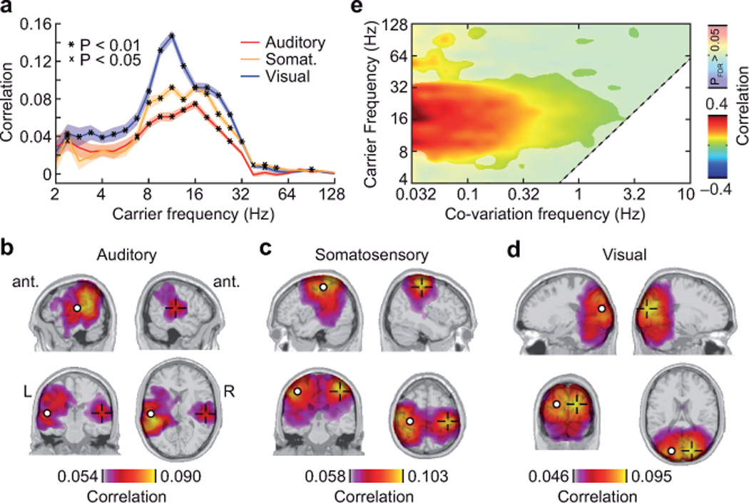
Power-envelope correlations between orthogonalized spontaneous signals from homologous early sensory areas. (a) Correlation between the auditory cortices (red), the somatosensory cortices (yellow), and the visual cortices (blue) resolved for carrier frequency. Colored bands indicate the s.e.m. across subjects. Spatial specificity is tested by comparison to the average correlation with the rest of the brain (one-tailed t-test; ^X for P < 0.05; * for P < 0.01). See Supplementary Figure 3a,b for a control analyses with different spectral smoothing. (b–d) Spatial distribution of the correlation between the left auditory b, somatosensory c, and visual d cortices and the rest of the brain. Correlation values are statistically masked (one-tailed t-test for correlation > average correlation with the rest of the brain, P < 0.05, FDR corrected for number of voxel). White circles indicate the location of the reference site; the crosses indicate the mirrored location in the other hemisphere. (e) Correlation between homologous sensory areas as a function of the carrier frequency and the co-variation frequency (center frequency of the ‘band-pass’ applied to the power envelopes before computing correlation on the second level). Note that the highest co-variation frequency is limited by the underlying carrier frequency (diagonal dashed line). The values are averaged across sensory modalities and subjects and are statistically masked (one-tailed t-test for correlation > average correlation to the rest of the brain, P < 0.05, FDR corrected for the number of carrier and co-variation frequencies). See Supplementary Figure 3c,d for control analyses with different spectral parameters.

We spectrally resolved the power envelope correlation (co-variation frequency; Fig. 2e) to assess its temporal scale. Correlation between homologous areas was significantly increased in a broad, low co-variation frequency range from 0.032 Hz (the lowest frequency analyzed) to above 1 Hz (one-sided t-test for correlation > average correlation, P < 0.05, FDR corrected). Thus, modulation of signal power on the time-scale of several seconds drove the correlation of spontaneous activity between sensory areas. These findings were insensitive to specific parameters of spectral analyses. We varied the spectral smoothing of the carrier- and the co-variation frequencies and obtained similar results (Supplementary Fig. 3). In summary, our analysis approach revealed that spontaneous oscillatory population activity in different homologous early sensory cortices was correlated on a slow time-scale in a spatially and spectrally specific manner.

Spatially specific correlation of higher-order cortices

We next extended our analysis beyond early sensory regions, and investigated how functional relations of higher-order cortices are reflected in power correlations. We characterized correlation maps of a higher visual area, a higher sensory-motor area and a prefrontal associative area for 16 Hz carrier frequency. The middle temporal area (MT+) is part of the dorsal visual pathway. Indeed, correlation with left and right MT+ did not only peak in the homologous area in the contralateral hemisphere, but also in the dorsal visual pathway along the intraparietal sulcus (Fig. 3a,b; one-sided t-test for correlation > average correlation, P < 0.05, FDR corrected). Correlation with the supplementary motor area (SMA), which is part of the sensory-motor cortex involved in planning of movements, peaked in frontal regions, that are compatible with the frontal eye fields and other regions in the parietal cortex (Fig. 3c; one-sided t-test for correlation > average correlation, P < 0.05, FDR corrected). Also the medial prefrontal cortex (MPFC), a higher-order associative area, exhibited spatially well-confined and symmetric correlation patterns (Fig. 3d; one-sided t-test for correlation > average correlation, P < 0.05, FDR corrected). Correlation with MPFC peaked in bilateral dorsal prefrontal cortex (DPFC) and bilateral lateral parietal cortex (LPC).

Figure 3.

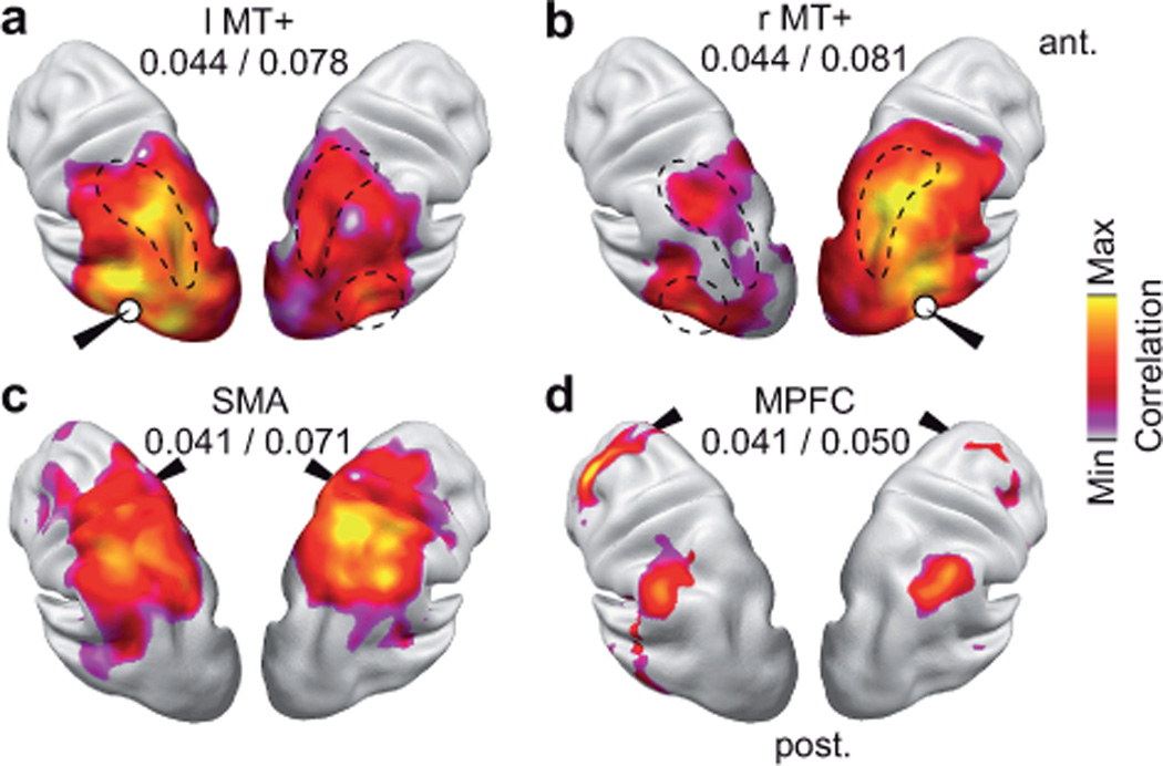
Correlation maps for selected locations at a carrier frequency of 16 Hz. Correlation maps are statistically masked (voxel-wise one-sided t-test for correlation > average correlation to the rest of the brain, P < 0.05, FDR corrected for the number of voxels). The white circles indicate the approximate location of the seeds. The values underneath the seed labels indicate the minimal and maximal correlation within the statistical mask. (a,b) Left and right middle temporal area (MT+). The homologous area in the other hemisphere and the intraparietal sulci are depicted by dashed lines. (c) Supplementary motor area (SMA). (d) Medial prefrontal cortex (MPFC).

The differences between correlation patterns of the above selected reference sites demonstrated that power-envelope correlations revealed distinct functional networks. However, the different correlation patterns also shared similar features. In particular, most reference sites showed a high correlation with parietal areas. This raised the question whether specific areas such as the parietal cortex might play a particularly prominent role in the global patterning of power envelope correlations. We next studied the correlation of power-envelopes across the full cortico-cortical space to address this question.

Global correlation structure

We derived the full connectivity matrix between 2,925 sources (nodes) that covered the brain in a regular 3D-grid. We defined a connection if the correlation between the orthogonalized signals of two sources was significantly higher than the average correlation of these sources to the rest of the brain (one-sided t-test, P < 0.01). We used graph-theoretical measures to quantify basic properties of the connectivity matrix³⁰. The number of connections (termed ‘degree’) was highest for the alpha and beta carrier-frequency range (8–32 Hz), where it reached about 25% of all possible connections (Fig. 4a). The spatial distribution of the degree for this carrier-frequency range was characterized by a global anterior to posterior increase (Fig. 4b). Besides this strong gradient, the degree distribution peaked prominently in bilateral LPC with significant connections to ~85% of all sources (MNI coordinates left: [–39 –54 32], right: [46 –45 39]).

Figure 4.

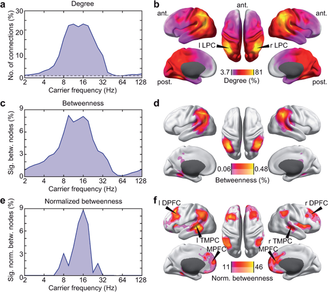
Graph-theoretical analysis of the global correlation structure of band-limited neuronal signals. (a) Spectrally resolved degree. The dashed line indicates the significance threshold (1.01%; P = 0.05, corrected for the number of nodes). (b) Degree at a carrier frequency of 16 Hz resolved in cortical space (LPC, lateral parietal cortex). The color scale is adjusted to the maximal and minimal degree occurring. (c) Spectrally resolved number of nodes with significantly increased betweenness compared to the average betweenness value (voxel-wise permutation test for betweenness > average betweenness, corrected for the number of nodes, P < 0.05). (d) Betweenness at a carrier frequency of 16 Hz resolved in cortical space. Betweenness is statistically masked at two levels (permutation test, corrected for the number of nodes, P < 0.05, saturated color scale; permutation test, P < 0.05, uncorrected, desaturated color scale). The color scale is adjusted to the maximal and minimal betweenness within the statistical mask. (e) Spectrally resolved number of normalized betweenness nodes defined analogously to c. (f) Normalized betweenness at a carrier frequency of 16 Hz resolved in cortical space defined analogously to d (MPFC, medial prefrontal cortex; TMPC, temporal cortex; DPFC, dorsal prefrontal cortex).

The prominent role of LPC was further supported by its high level of betweenness. Betweenness quantifies in how many of all possible shortest paths within a network a given node participates. It thus complements degree as a measure that quantifies a node's importance for mediating connectivity between other nodes, i.e. it’s ‘hubness’. For carrier frequencies in the alpha to beta frequency range (8–32 Hz), the number of significant betweenness nodes (permutation test, P < 0.05, corrected) and the spatial betweenness distribution qualitatively resembled the degree (Fig. 4c,d) with prominent maxima in bilateral LPC.

High degree favors high betweenness. Nodes with many connections are more likely to support the shortest paths between many other nodes. To account for this bias, we computed ‘normalized betweenness’, i.e. the betweenness corrected for betweenness that occurs in random networks with the same degree. In addition to LPC, this procedure exposed significant hubs in medial and bilateral dorsal prefrontal cortex (MNI coordinates MPFC: [10 60 10]; left DPFC: [–40 30 50], right DPFC: [30 20 30]) and bilateral temporal cortex (TMPC; MNI coordinates left: [–50 –40 –10], right: [60 –20 0]). The number of voxels with significant normalized betweenness peaked sharply at 16 Hz (Fig. 4e; permutation test, P < 0.05, corrected).

The pattern of connectivity at 16 Hz differed between the LPC, MPFC, DPFC, and TMPC. The high degree of bilateral LPC was driven by a widespread correlation with large parts of the brain (Fig. 5a,b; t-test for correlation > average correlation, P < 0.05, FDR corrected). The correlation was strongest to the vicinity of the LPC and to the LPC in the other hemisphere. By contrast, the hubs in bilateral MPFC, DPFC, and TMPC were characterized by sparser connectivity (Figs. 3d and 5c–f). Notably, most of the hub sites showed mutual peaks in the spatial correlation patterns. Thus, the LPC, MPFC, DPFC, and TMPC were not diffusely connected, but formed an interconnected network.

Figure 5.

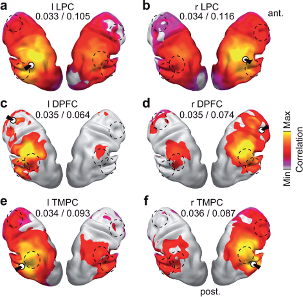
Correlation maps for identified hubs at a carrier frequency of 16 Hz. Correlation maps are statistically masked (voxel-wise one-sided t-test for correlation > average correlation to the rest of the brain, P < 0.05, FDR corrected for the number of voxels). The white circles indicate the approximate location of the hub that was used as reference for the correlation analysis. The dashed lines indicate the locations of the other hubs. The values underneath the seed labels indicate the minimal and maximal correlation within the statistical mask. (a,b) Left and right lateral parietal cortex (LPC). (c,d) Left and right dorsal prefrontal cortex (DPFC). (e,f) Left and right temporal cortex (TMPC).

Global correlation structure varies with carrier frequency

The above analyses focused on the carrier frequency of 16 Hz. To investigate if the global correlation structure varies across carrier frequencies, we performed a two-way analysis of variance (ANOVA) of the carrier-frequency dependent connectivity (4–45 Hz) with the factors carrier frequency and cortical location. Indeed, degree and betweenness showed significant main and interaction effects (Degree: main effect carrier frequency: F₇ = 4.88*10⁴, P = 0 main effect location F₂₉₂₄ = 102, P = 0, interaction: F_7,2924 = 9.88, P = 0; Betweenness: main effect carrier frequency: F₇ = 203, P = 5.15*10^–302, main effect location F₂₉₂₄ = 8.29, P = 0, interaction: F_7,2924 = 1.12, P = 8.01*10^–31). Thus, degree and betweenness were not only spatially inhomogeneous, but the spatial patterning of connectivity also depended on the underlying carrier frequency.

The frequency dependent degree revealed three prominent patterns of connectivity (Fig. 6). In the theta range (4–6 Hz), we found the highest degree in the medial temporal lobe (MTL, MNI coordinates, left: [–20 –40 –10], right: [40 –40 0]). In accordance with the above results, for frequencies in the alpha to beta frequency range (8–23 Hz), LPC showed the highest degree. In the low gamma frequency range (32–45 Hz), we found the highest degree in sensorimotor cortex (MNI coordinates left: [–40 –40 60], right: [40 –30 50]). These results were in close accordance with the patterns that we found for the frequency-dependent betweenness (Supplementary Fig. 4). In summary, the graph-theoretical analysis of global connectivity revealed spatially symmetric connectivity structure and localized hubs that depended on the underlying carrier frequency.

Figure 6.

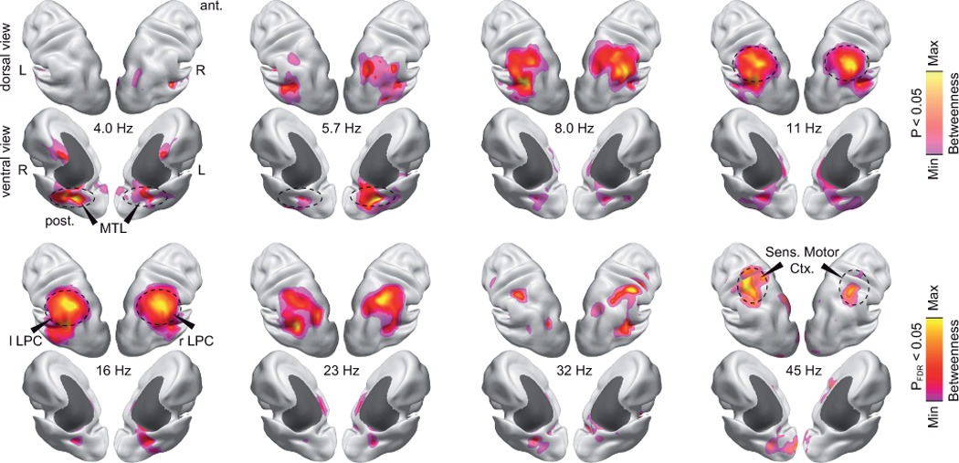
Spatial patterning of betweenness as a function of the carrier frequency. Betweenness values are statistically masked (voxel-wise permutation test for betweenness > average betweenness, corrected for number of nodes, P < 0.05, saturated color scale; P < 0.05, uncorrected, desaturated color scale). The color scale is adjusted to the minimal and maximal values within the statistical mask. Subcortical areas are masked dark gray. See Supplementary Figure 4 for complementary analysis of degree.

Discussion

In this study, we introduce a new analysis approach to characterize brain-wide functional connectivity based on power envelope correlation that overcomes limitations due to the limited spatial resolution of electrophysiological measures. Applying this approach to MEG, we provide a spectrally resolved characterization of the global organization of spontaneous electrophysiological signals in the human brain. The correlation of band-limited neuronal population activity showed prominent hubs that were largely symmetric across hemispheres and depended on the underlying carrier frequency.

Power envelope correlations between orthogonalized signals

Central for our findings was the new analysis approach for estimating power envelope correlations based on orthogonalized signals. In the present study, we applied this approach to MEG source estimates of spontaneous activity fluctuations of the resting human brain. However, because the underlying physical principles hold for both magnetic and electric fields, the approach should be similarly powerful for the analysis of EEG data. Furthermore, the approach is not limited to the analysis of spontaneous activity but may also provide new insights in task related functional connectivity. In general, the approach can be applied to any set of simultaneous electrophysiological signals to derive an index for functional connectivity, which may be relevant for bio-medical applications.

The combination of EEG or MEG with our analysis approach complements electrocorticogram (ECoG) recordings which have a higher spatial resolution and signal-to-noise ratio but are limited to a few focal sites and studies of the diseased brain^27,31,32. In fact, our analysis approach may also help investigating correlations between signals from nearby ECoG or microelectrode recordings that may also be affected by spurious correlation due to limited spatial resolution.

The applied analysis approach can provide a full connectivity matrix, which allows for studying brain wide correlation using graph theoretical methods. It is straightforward to apply this analysis approach also for contrasting groups of subjects or experimental conditions. The orthogonalization approach may also be combined with multivariate methods such as independent component analysis (ICA) to identify networks of areas with correlated power envelopes²⁹. Furthermore, also non-linear or directed measures of interaction may be applied to the power envelopes of orthogonalized signals.

The global correlation depends on the carrier frequency

We found that the global correlation of spontaneous activity peaked for carrier frequencies in the alpha to beta range with prominent hubs in the LPC and secondary hubs in PFC and TMPC. These hubs resemble the hub structures reported for spontaneous hemodynamic signals⁸. We found that all these hubs were not diffusely connected but were strongly correlated with each other as a global network. This network structure is compatible with the spatial pattern extracted from spontaneous MEG power fluctuations in the alpha to beta band using ICA²⁹. The identified network overlaps with two networks in the correlation of hemodynamic signals: The ‘default mode network’^2,3,33, which comprises areas typically deactivated during tasks, and a ‘control network’^5,7, which has been implicated in executive functions. Besides this global structure, for the same alpha to beta carrier-frequency range, our analysis revealed spatially distinct correlations between functionally related sensory and associative cortices. These results substantiate converging evidence from MEG^{28,29,34–36} and EEG^37–39 of the resting brain that suggest a prominent correlation of oscillatory power in particular in the alpha to beta frequency range. Thus, correlation of alpha to beta activity may be a generic signature of intrinsic neuronal interactions.

In addition to the prominent effects in the alpha to beta band, we found spatially specific correlation structure of spontaneous activity for a wide range of carrier frequencies from the theta to the gamma band (4–45 Hz). In the theta frequency range (4–6 Hz) the MTL constituted a global hub. Theta-band oscillations are a prominent feature of neuronal dynamics in the MTL. They seem tightly related to memory processes and are phase-coupled to neuronal activity in other cortical regions^40–42. Also studies of fMRI connectivity identified ‘mnemonic networks’ that involve the MTL^4,6. In accordance with these findings, our results suggest that the MTL is central to the brain-wide co-variation of spontaneous theta-band activity.

Timescale of power envelope correlations

In accordance with other MEG^28,35,36 and intracranial recordings^27,43, we found that correlations of oscillatory power were driven by slow co-variations in a broad frequency range below 0.1 Hz. Similarly, hemodynamic correlations are dominated by frequencies below 0.1 Hz²⁶. These slow co-fluctuations may arise from intrinsic cortical dynamics⁴⁴ and subcortical or neuromodulatory inputs^18,19,43,45. The slow time scale of power envelope correlations contrasts with the millisecond timescale of neuronal signaling itself. Power envelope correlations likely reflect the consequence of signaling rather than being a mechanism that controls the signaling on a fast time-scale.

Relation to local neuronal activity

In the raw EEG or MEG of awake humans, alpha and beta oscillations are the most prominent rhythms. One could speculate that the strong correlations in the alpha and beta frequency range simply reflect the better signal-to-noise ratio of these prominent local signals. However, differences in the spatial characteristics argue against this explanation. Local alpha and beta oscillations appear widespread across occipital, parietal, and central areas (Supplementary Fig. 5). This pattern differs substantially from the global hub structure that we identified within this frequency range based on power-envelope correlations (cf. Fig. 6). Also at other frequencies, the hub structure differs substantially from the spatial distribution of local signal power. Thus, the strength of local oscillatory processes and their brain-wide spatial correlation are dissociated. Consequently, the correlation of signal power may provide complementary information to local signal power that could be exploited in future applications.

Relation to fMRI

EEG and MEG allow for separating neuronal activity into oscillatory components that reflect the biophysical properties of different local and large-scale network processes^17–19. By contrast, fMRI provides a compound measure of the joint metabolic cost of different network processes and of non-neuronal processes^14–16,18. This compound nature of the hemodynamic signal is reflected in its correlation with oscillatory neuronal activity across a broad range of frequencies during stimulation^46–48 and at rest^{37–39,45,49}. Thus, the correlation structure of electrophysiological and hemodynamic signals should share similarities. Indeed, the patterning and the time scale of electrophysiological signal correlation that we found showed substantial similarities with fMRI connectivity (see above).

However, despite these similarities, the spatial structure of power-envelope correlations also exhibited differences to hemodynamic correlation. In particular, hemodynamic correlation is characterized by prominent hubs in the posterior midline^2,8,33, which were largely absent in the electrophysiological connectivity reported here and in networks extracted from MEG using ICA²⁹. This apparent discrepancy may reflect the different nature of electrophysiological and hemodynamic signals. Furthermore, it should be taken into account that source estimates from EEG and MEG may have a spatially inhomogeneous sensitivity, which might result in an attenuation of deep sources.

Power envelope correlation in the gamma frequency range

Neuronal oscillations in the gamma frequency range have been found in various experimental contrasts and may be a generic signature of local cortical activity^18,22. A growing number of combined electrophysiology and fMRI studies has linked hemodynamic signals to neuronal activity in particular in the gamma band^{45,46,48–50}. These findings suggests, that resting state functional connectivity known from fMRI² may manifest in the correlation of oscillatory activity in the gamma frequency range. This notion is supported by invasive ECoG studies that found long-range power correlation within this frequency range^27,31,32.

In contrast, we did not find prominent global correlation in the gamma frequency range. This seemingly unexpected finding may relate to different issues. First, the source of variance that drives the neuronal signals likely has a profound influence¹⁸. Sensory stimulation effectively drives cortical gamma-band activity^18,46 that can be measured with EEG and MEG^21,23,48. By contrast, during rest, gamma-band fluctuations may be much smaller and the global correlation may be dominated by alpha to beta-band activity. Second, the spatial sampling of recorded signals likely plays an important role. Compared to intracranial electrodes, EEG and MEG average over larger populations of neurons. As a consequence, EEG and MEG may be particularly sensitive to spectral components with a broader spatial coherence, while intracranial measures may be more sensitive to locally coherent rhythms. Non-invasive and invasive measures may thus emphasize signals with different spatial and spectral characteristics.

Methods

Methods and any associated references are available in the online version of the paper at http://www.nature.com/natureneuroscience/.

Online Methods

MEG Recording

MEG was continuously recorded with a 275-channel whole-head system (Omega 2000, CTF Systems Inc., Port Coquitlam, Canada) in a magnetically shielded room. The electro-oculogram (EOG) was recorded simultaneously for off-line artifact rejection. The head position relative to the MEG sensors was measured continuously using a set of head localization coils (nasion, left and right ears). MEG signals were low-pass filtered online (cutoff: 300 Hz) and recorded with a sampling rate of 1,200 Hz.

Subjects and Experimental Procedure

Subjects (n = 43; age: 25.5 ± 3.5 years, mean ± s.d.; 21 females) fixated a cross projected centrally onto a back projection screen with an LCD projector (Sanyo Pro Xtrax PLC-XP51, Sanyo, Japan) from outside the magnetically shielded room. Subjects were instructed to continuously maintain fixation (duration: 505 ± 115 s, mean ± s.d.; 360–620 s, range). The study was conducted in accordance with the Declaration of Helsinki and informed consent was obtained from all participants prior to the recordings.

Preprocessing and Artifact Rejection

The data were high-pass filtered offline (cut-off: 0.5 Hz, Butterworth, 4^th order) and artifactual data (eye movements, strong muscle activity) were rejected based on visual inspection (13.4 ± 7.6 %, mean ± s.d.; 2.1–39.5 %, range). For the analysis of spectral components above 32 Hz, we performed additional cleaning to account for muscular artifacts. The data were high-pass filtered (30 Hz, Butterworth, 4^th order), independent component analysis was computed, and artifactual components related to muscular activity were rejected from the data (7 ± 3.8, mean ± s.d.; 1–16, range).

Analysis software

All data analyses were performed in Matlab (MathWorks, Natick, MA, USA) using custom scripts and open source toolboxes: Fieldtrip⁵¹ (http://www.ru.nl/fcdonders/fieldtrip/), SPM2 (http://www.fil.ion.ucl.ac.uk/spm/), Brain Connectivity Toolbox³⁰ (http://www.brain-connectivity-toolbox.net/).

Spectral Analysis

We derived spectral estimates using Morlet’s wavelets⁵² w(t,f):

$$w(t,f)={\left({\sigma }_t\sqrt{\pi }\right)}^{-1/2}{e}^{-t/2{\sigma }_t^2}{e}^{-i2\pi ft}$$

Here, f is the center frequency (carrier frequency) and σ_t is the temporal s.d.. The time-frequency estimate X(f,t) of a signal x(t) was then computed by convolution with w(t,f):

$$X(t,f)=x(t)*w(t,f)$$

We chose a spectral band-width of 1/2 octaves (corresponding to f/σ_f ~ 5.83; σ_f, spectral s.d.) and spaced the center frequencies logarithmically according to the exponentiation of the base 2 with exponents ranging from 1 to 7 in steps of 1/4. We derived spectral estimates in successive half overlapping temporal windows that covered ±3 σ_t. For time points, where the convolution kernel overlapped with sections marked as artifacts (see preprocessing) the data were discarded.

Source Locations and Physical Forward Model

For source analyses, we used three different source configurations defined in MNI space: (1) For correlation maps of selected reference locations, spatial normalization of correlation values for statistical testing (see below), and the all-to-all analysis, we used a regular 3D grid that covered the whole brain (1 cm spacing, 2,925 source locations; for co-variation frequency analyses we used 2 cm spacing, 369 source locations). (2) For the correlation analysis between homologous sensory areas, we defined bilateral sensory locations in MNI space. The coordinates of the sensory regions were identified by a meta-analysis of fMRI literature using the BrainMap.org resources⁵³. Locations: auditory cortex ([–54 –22 10], [52 –24 12]), somatosensory cortex ([–42 –26 54], [38 –32 48]), visual cortex ([–20 –86 18], [16 –80 26]). (3) Locations of interest derived from fMRI correlation literature³ for seed correlation analyses: l/r MT+ (MNI coordinates: [–47 –69 –3], [54 –63 –8]), MPFC (MNI coordinate: [–3 39 –2]), SMA (MNI coordinate: [–2 1 51]).

For source analysis, we constructed individual physical forward models (leadfields). We affine transformed source locations into individual head space using the participants’ individual T1-weighted structural MRI and aligned the MEG sensors to the head geometry based on 3 fiducial points (nasion, left and right ear, registered during the MEG acquisition by 3 head localization coils). To derive the physical relation between sources and sensors, we employed a single shell model⁵⁴.

Source Analysis

We used adaptive linear spatial filtering (beamforming)^23,55,56 to estimate the spectral amplitude and phase of neuronal signals at the source level.

The implementation details of the beamformer were as follows: For each frequency f and source location r, 3 orthogonal filters (Â=[A₁, A₂, A₃]; one for each spatial dimension) were computed that pass activity from location r with unit gain, while maximally suppressing activity from all other sources:

$$\widehat{A}(r,f)={[L^T(r)C_{\mathit{\text{real}}}{(f)}^{-1}L(r)]}^{-1}{L}^T(r)C_{\mathit{\text{real}}}{(f)}^{-1}$$

Here, L(r) is a matrix whose columns are the leadfields of three orthogonal dipoles at source location r, and C_real denotes the real part of the complex cross-spectral-density matrix for the sensor level data at frequency f, and ^T indicates the matrix transpose. We linearly combined the 3 filters to a single filter pointing in the direction of maximal variance, i.e. the dominant dipole orientation. To this end, the filters were weighted with the first eigenvectors’ elements (the eigenvector with the largest eigenvalue of the real part of the cross-spectral-density matrix at the source location r):

$$\begin{array}{c}\nu (r,f)=[{\nu }_1(r,f),{\nu }_2(r,f),{\nu }_3(r,f)]=Ei{g}_1(\widehat{A}(r,f)C_{\mathit{\text{real}}}(f)\widehat{A}{(r,f)}^{*T})\\ A(r,f)={\nu }_1(r,f){\widehat{A}}_1(r,f)+{\nu }_2(r,f){\widehat{A}}_2(r,f)+{\nu }_3(r,f){\widehat{A}}_3(r,f)\end{array}$$

To derive the complex source estimates, the complex frequency domain data were then multiplied with the real-valued filter:

$$X_{\mathit{\text{source}}}(r,t,f)=A(r,f)X_{\mathit{\text{sensor}}}(t,f)$$

Here, X_sensor(t,f) is the frequency domain representation of the sensor level data at time t and frequency f, and X_source(r,t,f) is the corresponding source signal at location r. To account for the spatial bias of the beamforming solution when investigating signal power (Supplementary Fig. 5), we jointly normalized the three leadfields for each source location by division with the sum of all squared values.

Power Envelope Correlation between Orthogonalized Signals

Here we provide a brief account of the applied method. Please see Supplementary Data and Supplementary Figures 1 and 2 for additional information and numerical simulations on this approach.

We assessed neuronal interactions by quantifying correlations between power envelopes^19,20,57,58. To this end, we squared the absolute values of the complex spectral estimates and applied a logarithmic transform to render the power statistics more normal. We then computed Pearson’s linear correlation between the resulting power envelopes from two different locations.

To discount spurious correlations caused by the limited spatial resolution of source estimates, we orthogonalized any two time series of band-limited activity before computing their power envelopes. We performed this operation in the frequency domain. We defined the complex signal Y(t,f) orthogonalized to the complex signal X(t,f) (see Supplementary Fig. 1):

$$Y_{\perp X}(t,f)=\mathit{\text{imag}}(Y(t,f)\frac{X{(t,f)}^{*}}{|X(t,f)|})$$

The orthogonalization can be done in two directions (X to Y, Y to X). We computed power envelope correlations for both directions of orthogonalized time-series and averaged the values for subsequent analysis. We performed the orthogonalization time-point by time-point, which requires no assumption about stationary of the signals’ relation beyond the length of the carrier-frequency dependent analysis window. Discounting the non-orthogonal signal components leads to an underestimation of true correlation by a factor of ~0.577. This factor was accounted for when reporting correlation values between orthogonalized signals.

Spectrally Resolved Correlation of Power Envelopes (2^nd Level Analysis)

To resolve the correlation between two orthogonalized signals in frequency (co-variation frequency) we applied spectral analysis to the power envelopes with an approach equivalent to using Morlet’s wavelets. We chose a spectral bandwidth of 0.95 octaves (f/σ_f ~ 3.15) and spaced the center frequencies logarithmically according to the exponentiation of the base 10 with exponents ranging from –1.5 in steps of 0.1 to 1/6 of the carrier frequency. We derived spectral estimates in successive half overlapping temporal windows that covered ±3 σ_t. From these complex numbers we derived the coherency between power envelopes and took the real part of coherency as the frequency specific measure of correlation.

Power envelopes were interrupted by periods of missing data due to artifacts such as eye blinks or strong muscle activity. Thus, the convolution with Morlet’s wavelets as described above was not feasible and we employed a spectral estimate approach that could cope with missing data. For discrete signals time domain and frequency domain representations are linearly related:

$$\begin{array}{cc}x=BX,& X=\mathit{\text{inv}}(B)x\end{array}$$

Here, x is the time domain representation, X is the frequency domain representation, and B is the Fourier basis (i.e. family of orthogonal complex sinusoids). For data with invalid temporal sections B is rank deficient. In this case we derived the spectral estimate employing the pseudo inverse.

$$X=\mathit{\text{pinv}}(B)x$$

As a windowing function we used a Gaussian taper such that if no data was missing the approach was identical to using Morlet’s wavelets. Data sections with more than 50% missing data were discarded from the analysis.

Statistical Analysis of Correlation Structure and Definition of ‘Connections’

Across a broad range of frequencies, power-envelope correlations between orthogonalized signals had a positive offset, i.e. the brain-wide correlation was consistently larger than zero. To focus on the spatial correlation structure, we used Student’s t-tests and identified correlation higher than the average correlation to all locations on a 3D grid covering the brain. We corrected for multiple comparisons by controlling the false discovery rate (FDR). Please note that this statistic depends on the sources across which the average correlation is estimated.

For the analysis of the global correlation structure, no particular reference location exists. For this case, the correlation between any two sites can statistically be compared to the brain-wide correlation of either one of the two sites. We established a symmetric connectivity measure by defining a connection to be present if statistics for either one of the two possible normalizations reached significance (we accounted for two tests by Bonferroni correction; P_Threshold = 0.01/2). This resulted in a symmetric connection matrix that was used for subsequent graph theoretical analyses. The symmetrization allowed for fully connected nodes, in other words, there could be more than 50% connections (e.g. see Fig. 4b).

Graph Theoretical Analysis

We used graph theoretical measures³⁰ to quantify basic properties of global connectivity. We employed three measures highlighting different aspects of the global correlation:

Degree:

$$D_i=\frac{1}{N-1}\sum _j{a}_{ij}$$

Here, D_i is the ‘degree’ at location i, and a_ij is the connection (0 for no connection, 1 for a connection) between locations i and j, and N is the total number of connections. The total degree is the average of the degree at all locations.

Betweenness:

$$B_i=\frac{1}{(N-1)(N-2)}\sum _{\begin{array}{c}h,j\\ h\ne i,h\ne j,j\ne i\end{array}}\frac{{\rho }_{hj}(i)}{{\rho }_{hj}}$$

Here, B_i is the ‘betweenness’ at location i, and ρ_hj is the number of shortest paths between h and j, and ρ_hj(i) is the number of shortest paths between h and j that passes through i.

Normalized betweenness:

$$B{N}_i=\frac{B_i-\mathit{\text{mean}}(B_i^{\mathit{\text{rand}}})}{sd(B_i^{\mathit{\text{rand}}})}$$

Here, BN_i is the ‘normalized betweenness’ at location i derived from the betweenness B_i and the mean mean( ) and standard deviation sd( ) of a set of betweenness values B_i^rand (20 resamples) from connection matrices with identical degree but randomized connectivity⁵⁹. Thus, normalized betweenness accounts for the betweenness that occurs in a random network with identical degree.

Statistical Analysis of Graph-theoretical Measures

We performed random effects statistics to assess the modulation of graph-theoretical measures. We first derived single subject estimates of graph-theoretical measures using a jackknifing procedure: For each subject i of N subjects we derived a robust jackknife resample R_i by averaging graph-theoretical measures from connectivity matrices based on all but this subject and one other subject at a time. From these jackknife resamples we computed single subject estimates G_i.

$$G_i=\sum _{j=1}^N{R}_j-(N-1)R_i$$

This corresponds to pseudo-values without bias correction. Based on these estimates, we performed the following random-effects statistics.

To assess the spatial patterning of graph-theoretical measures, we employed random permutation statistics. We generated an empirical null hypothesis distribution for no spatial patterns by randomly permuting source locations for each subject and then computing the average across subjects (10,000 resamples). We selected only the largest value across the entire space of each resample to account for multiple testing. To assess the modulation of graph-theoretical measures with the factors carrier frequency and spatial location and their interaction we performed a two-way analysis of variance (ANOVA).

Illustration of results

To illustrate the spatial distribution of correlation and graph-theoretical measures, we projected the quantities onto the cortical surface from the Population-Average, Landmark- and Surface-based (PALS) atlas⁶⁰ or alternatively as an overlay on brain slices of the SPM99/2 template brain. We used different statistical masks as explained in the corresponding figure legends.

References

- 1.Biswal B, Yetkin FZ, Haughton VM, Hyde JS. Functional connectivity in the motor cortex of resting human brain using echo-planar MRI. Magn Reson Med. 1995;34:537–541. doi: 10.1002/mrm.1910340409. [DOI] [PubMed] [Google Scholar]
- 2.Fox MD, Raichle ME. Spontaneous fluctuations in brain activity observed with functional magnetic resonance imaging. Nat. Rev. Neurosci. 2007;8:700–711. doi: 10.1038/nrn2201. [DOI] [PubMed] [Google Scholar]
- 3.Fox MD, et al. The human brain is intrinsically organized into dynamic, anticorrelated functional networks. Proc. Natl. Acad. Sci. U.S.A. 2005;102:9673–9678. doi: 10.1073/pnas.0504136102. [DOI] [PMC free article] [PubMed] [Google Scholar]
- 4.Vincent JL, et al. Coherent spontaneous activity identifies a hippocampal-parietal memory network. J. Neurophysiol. 2006;96:3517–3531. doi: 10.1152/jn.00048.2006. [DOI] [PubMed] [Google Scholar]
- 5.Vincent JL, Kahn I, Snyder AZ, Raichle ME, Buckner RL. Evidence for a frontoparietal control system revealed by intrinsic functional connectivity. J. Neurophysiol. 2008;100:3328–3342. doi: 10.1152/jn.90355.2008. [DOI] [PMC free article] [PubMed] [Google Scholar]
- 6.Kahn I, Andrews-Hanna JR, Vincent JL, Snyder AZ, Buckner RL. Distinct cortical anatomy linked to subregions of the medial temporal lobe revealed by intrinsic functional connectivity. J. Neurophysiol. 2008;100:129–139. doi: 10.1152/jn.00077.2008. [DOI] [PMC free article] [PubMed] [Google Scholar]
- 7.Dosenbach NUF, et al. Distinct brain networks for adaptive and stable task control in humans. Proc. Natl. Acad. Sci. U.S.A. 2007;104:11073–11078. doi: 10.1073/pnas.0704320104. [DOI] [PMC free article] [PubMed] [Google Scholar]
- 8.Buckner RL, et al. Cortical hubs revealed by intrinsic functional connectivity: mapping, assessment of stability, and relation to Alzheimer’s disease. J. Neurosci. 2009;29:1860–1873. doi: 10.1523/JNEUROSCI.5062-08.2009. [DOI] [PMC free article] [PubMed] [Google Scholar]
- 9.Power JD, et al. Functional Network Organization of the Human Brain. Neuron. 2011;72:665–678. doi: 10.1016/j.neuron.2011.09.006. [DOI] [PMC free article] [PubMed] [Google Scholar]
- 10.Lewis CM, Baldassarre A, Committeri G, Romani GL, Corbetta M. From the Cover: Learning sculpts the spontaneous activity of the resting human brain. Proceedings of the National Academy of Sciences. 2009;106:17558–17563. doi: 10.1073/pnas.0902455106. [DOI] [PMC free article] [PubMed] [Google Scholar]
- 11.Dehaene S, Changeux J-P. Experimental and theoretical approaches to conscious processing. Neuron. 2011;70:200–227. doi: 10.1016/j.neuron.2011.03.018. [DOI] [PubMed] [Google Scholar]
- 12.Zhang D, Raichle ME. Disease and the brain’s dark energy. Nat Rev Neurol. 2010;6:15–28. doi: 10.1038/nrneurol.2009.198. [DOI] [PubMed] [Google Scholar]
- 13.Hawellek DJ, Hipp JF, Lewis CM, Corbetta M, Engel AK. Increased functional connectivity indicates the severity of cognitive impairment in multiple sclerosis. Proceedings of the National Academy of Sciences. 2011 doi: 10.1073/pnas.1110024108. [DOI] [PMC free article] [PubMed] [Google Scholar]
- 14.Logothetis NK. What we can do and what we cannot do with fMRI. Nature. 2008;453:869–878. doi: 10.1038/nature06976. [DOI] [PubMed] [Google Scholar]
- 15.Sirotin YB, Das A. Anticipatory haemodynamic signals in sensory cortex not predicted by local neuronal activity. Nature. 2009;457:475–479. doi: 10.1038/nature07664. [DOI] [PMC free article] [PubMed] [Google Scholar]
- 16.Heeger DJ, Ress D. What does fMRI tell us about neuronal activity? Nat. Rev. Neurosci. 2002;3:142–151. doi: 10.1038/nrn730. [DOI] [PubMed] [Google Scholar]
- 17.Wang X-J. Neurophysiological and computational principles of cortical rhythms in cognition. Physiol. Rev. 2010;90:1195–1268. doi: 10.1152/physrev.00035.2008. [DOI] [PMC free article] [PubMed] [Google Scholar]
- 18.Donner TH, Siegel M. A framework for local cortical oscillation patterns. Trends Cogn. Sci. (Regul. Ed.) 2011;15:191–199. doi: 10.1016/j.tics.2011.03.007. [DOI] [PubMed] [Google Scholar]
- 19.Siegel M, Donner TH, Engel AK. Spectral fingerprints of large-scale neuronal interactions. Nat. Rev. Neurosci. 2012;13:121–134. doi: 10.1038/nrn3137. [DOI] [PubMed] [Google Scholar]
- 20.Bruns A, Eckhorn R, Jokeit H, Ebner A. Amplitude envelope correlation detects coupling among incoherent brain signals. Neuroreport. 2000;11:1509–1514. [PubMed] [Google Scholar]
- 21.Siegel M, Donner TH, Oostenveld R, Fries P, Engel AK. Neuronal synchronization along the dorsal visual pathway reflects the focus of spatial attention. Neuron. 2008;60:709–719. doi: 10.1016/j.neuron.2008.09.010. [DOI] [PubMed] [Google Scholar]
- 22.Fries P. Neuronal gamma-band synchronization as a fundamental process in cortical computation. Annu. Rev. Neurosci. 2009;32:209–224. doi: 10.1146/annurev.neuro.051508.135603. [DOI] [PubMed] [Google Scholar]
- 23.Hipp JF, Engel AK, Siegel M. Oscillatory synchronization in large-scale cortical networks predicts perception. Neuron. 2011;69:387–396. doi: 10.1016/j.neuron.2010.12.027. [DOI] [PubMed] [Google Scholar]
- 24.Nolte G, et al. Identifying true brain interaction from EEG data using the imaginary part of coherency. Clin Neurophysiol. 2004;115:2292–2307. doi: 10.1016/j.clinph.2004.04.029. [DOI] [PubMed] [Google Scholar]
- 25.Schoffelen J-M, Gross J. Source connectivity analysis with MEG and EEG. Hum Brain Mapp. 2009;30:1857–1865. doi: 10.1002/hbm.20745. [DOI] [PMC free article] [PubMed] [Google Scholar]
- 26.Cordes D, et al. Frequencies contributing to functional connectivity in the cerebral cortex in ‘resting-state’ data. AJNR Am J Neuroradiol. 2001;22:1326–1333. [PMC free article] [PubMed] [Google Scholar]
- 27.Nir Y, et al. Interhemispheric correlations of slow spontaneous neuronal fluctuations revealed in human sensory cortex. Nat. Neurosci. 2008;11:1100–1108. doi: 10.1038/nn.2177. [DOI] [PMC free article] [PubMed] [Google Scholar]
- 28.Brookes MJ, et al. Measuring functional connectivity using MEG: Methodology and comparison with fcMRI. Neuroimage. 2011;56:1082–1104. doi: 10.1016/j.neuroimage.2011.02.054. [DOI] [PMC free article] [PubMed] [Google Scholar]
- 29.Brookes MJ, et al. Investigating the electrophysiological basis of resting state networks using magnetoencephalography. Proceedings of the National Academy of Sciences. 2011 doi: 10.1073/pnas.1112685108. [DOI] [PMC free article] [PubMed] [Google Scholar]
- 30.Rubinov M, Sporns O. Complex network measures of brain connectivity: uses and interpretations. Neuroimage. 2010;52:1059–1069. doi: 10.1016/j.neuroimage.2009.10.003. [DOI] [PubMed] [Google Scholar]
- 31.He BJ, Snyder AZ, Zempel JM, Smyth MD, Raichle ME. Electrophysiological correlates of the brain’s intrinsic large-scale functional architecture. Proc. Natl. Acad. Sci. U.S.A. 2008;105:16039–16044. doi: 10.1073/pnas.0807010105. [DOI] [PMC free article] [PubMed] [Google Scholar]
- 32.Miller KJ, Weaver KE, Ojemann JG. Direct electrophysiological measurement of human default network areas. Proc. Natl. Acad. Sci. U.S.A. 2009;106:12174–12177. doi: 10.1073/pnas.0902071106. [DOI] [PMC free article] [PubMed] [Google Scholar]
- 33.Greicius MD, Krasnow B, Reiss AL, Menon V. Functional connectivity in the resting brain: a network analysis of the default mode hypothesis. Proc. Natl. Acad. Sci. U.S.A. 2003;100:253–258. doi: 10.1073/pnas.0135058100. [DOI] [PMC free article] [PubMed] [Google Scholar]
- 34.Bassett DS, Meyer-Lindenberg A, Achard S, Duke T, Bullmore E. Adaptive reconfiguration of fractal small-world human brain functional networks. Proc. Natl. Acad. Sci. U.S.A. 2006;103:19518–19523. doi: 10.1073/pnas.0606005103. [DOI] [PMC free article] [PubMed] [Google Scholar]
- 35.Liu Z, Fukunaga M, de Zwart JA, Duyn JH. Large-scale spontaneous fluctuations and correlations in brain electrical activity observed with magnetoencephalography. Neuroimage. 2010;51:102–111. doi: 10.1016/j.neuroimage.2010.01.092. [DOI] [PMC free article] [PubMed] [Google Scholar]
- 36.de Pasquale F, et al. Temporal dynamics of spontaneous MEG activity in brain networks. Proc. Natl. Acad. Sci. U.S.A. 2010;107:6040–6045. doi: 10.1073/pnas.0913863107. [DOI] [PMC free article] [PubMed] [Google Scholar]
- 37.Laufs H, et al. Electroencephalographic signatures of attentional and cognitive default modes in spontaneous brain activity fluctuations at rest. Proc. Natl. Acad. Sci. U.S.A. 2003;100:11053–11058. doi: 10.1073/pnas.1831638100. [DOI] [PMC free article] [PubMed] [Google Scholar]
- 38.Mantini D, Perrucci MG, Del Gratta C, Romani GL, Corbetta M. Electrophysiological signatures of resting state networks in the human brain. Proc. Natl. Acad. Sci. U.S.A. 2007;104:13170–13175. doi: 10.1073/pnas.0700668104. [DOI] [PMC free article] [PubMed] [Google Scholar]
- 39.Jann K, Kottlow M, Dierks T, Boesch C, Koenig T. Topographic electrophysiological signatures of FMRI resting state networks. PLoS ONE. 2010;5 doi: 10.1371/journal.pone.0012945. [DOI] [PMC free article] [PubMed] [Google Scholar]
- 40.Buzsáki G. Theta oscillations in the hippocampus. Neuron. 2002;33:325–340. doi: 10.1016/s0896-6273(02)00586-x. [DOI] [PubMed] [Google Scholar]
- 41.Fell J, Axmacher N. The role of phase synchronization in memory processes. Nat. Rev. Neurosci. 2011;12:105–118. doi: 10.1038/nrn2979. [DOI] [PubMed] [Google Scholar]
- 42.Battaglia FP, Benchenane K, Sirota A, Pennartz CMA, Wiener SI. The hippocampus: hub of brain network communication for memory. Trends Cogn. Sci. (Regul. Ed.) 2011;15:310–318. doi: 10.1016/j.tics.2011.05.008. [DOI] [PubMed] [Google Scholar]
- 43.Leopold DA, Murayama Y, Logothetis NK. Very slow activity fluctuations in monkey visual cortex: implications for functional brain imaging. Cereb. Cortex. 2003;13:422–433. doi: 10.1093/cercor/13.4.422. [DOI] [PubMed] [Google Scholar]
- 44.Deco G, Jirsa VK, McIntosh AR. Emerging concepts for the dynamical organization of resting-state activity in the brain. Nat Rev Neurosci. 2011;12:43–56. doi: 10.1038/nrn2961. [DOI] [PubMed] [Google Scholar]
- 45.Schölvinck ML, Maier A, Ye FQ, Duyn JH, Leopold DA. Neural basis of global resting-state fMRI activity. Proc. Natl. Acad. Sci. U.S.A. 2010;107:10238–10243. doi: 10.1073/pnas.0913110107. [DOI] [PMC free article] [PubMed] [Google Scholar]
- 46.Logothetis NK, Pauls J, Augath M, Trinath T, Oeltermann A. Neurophysiological investigation of the basis of the fMRI signal. Nature. 2001;412:150–157. doi: 10.1038/35084005. [DOI] [PubMed] [Google Scholar]
- 47.Goense JBM, Logothetis NK. Neurophysiology of the BOLD fMRI signal in awake monkeys. Curr. Biol. 2008;18:631–640. doi: 10.1016/j.cub.2008.03.054. [DOI] [PubMed] [Google Scholar]
- 48.Scheeringa R, et al. Neuronal Dynamics Underlying High- and Low-Frequency EEG Oscillations Contribute Independently to the Human BOLD Signal. Neuron. 2011;69:572–583. doi: 10.1016/j.neuron.2010.11.044. [DOI] [PubMed] [Google Scholar]
- 49.Magri C, Schridde U, Murayama Y, Panzeri S, Logothetis NK. The Amplitude and Timing of the BOLD Signal Reflects the Relationship between Local Field Potential Power at Different Frequencies. J. Neurosci. 2012;32:1395–1407. doi: 10.1523/JNEUROSCI.3985-11.2012. [DOI] [PMC free article] [PubMed] [Google Scholar]
- 50.Mukamel R, et al. Coupling between neuronal firing, field potentials, and FMRI in human auditory cortex. Science. 2005;309:951–954. doi: 10.1126/science.1110913. [DOI] [PubMed] [Google Scholar]
- 51.Oostenveld R, Fries P, Maris E, Schoffelen J-M. FieldTrip: Open source software for advanced analysis of MEG, EEG, and invasive electrophysiological data. Comput Intell Neurosci. 2011;2011:156869. doi: 10.1155/2011/156869. [DOI] [PMC free article] [PubMed] [Google Scholar]
- 52.Tallon-Baudry C, Bertrand O, Delpuech C, Pernier J. Stimulus specificity of phase-locked and non-phase-locked 40 Hz visual responses in human. J. Neurosci. 1996;16:4240–4249. doi: 10.1523/JNEUROSCI.16-13-04240.1996. [DOI] [PMC free article] [PubMed] [Google Scholar]
- 53.Laird AR, et al. ALE Meta-Analysis Workflows Via the Brainmap Database: Progress Towards A Probabilistic Functional Brain Atlas. Front Neuroinformatics. 2009;3:23. doi: 10.3389/neuro.11.023.2009. [DOI] [PMC free article] [PubMed] [Google Scholar]
- 54.Nolte G. The magnetic lead field theorem in the quasi-static approximation and its use for magnetoencephalography forward calculation in realistic volume conductors. Phys Med Biol. 2003;48:3637–3652. doi: 10.1088/0031-9155/48/22/002. [DOI] [PubMed] [Google Scholar]
- 55.Van Veen BD, van Drongelen W, Yuchtman M, Suzuki A. Localization of brain electrical activity via linearly constrained minimum variance spatial filtering. IEEE Trans Biomed Eng. 1997;44:867–880. doi: 10.1109/10.623056. [DOI] [PubMed] [Google Scholar]
- 56.Gross J, et al. Dynamic imaging of coherent sources: Studying neural interactions in the human brain. Proc. Natl. Acad. Sci. U.S.A. 2001;98:694–699. doi: 10.1073/pnas.98.2.694. [DOI] [PMC free article] [PubMed] [Google Scholar]
- 57.Schepers IM, Hipp JF, Schneider TR, Röder B, Engel AK. Functionally specific oscillatory activity correlates between visual and auditory cortex in the blind. Brain. 2012;135:922–934. doi: 10.1093/brain/aws014. [DOI] [PubMed] [Google Scholar]
- 58.Donner TH, Siegel M, Fries P, Engel AK. Buildup of choice-predictive activity in human motor cortex during perceptual decision making. Curr. Biol. 2009;19:1581–1585. doi: 10.1016/j.cub.2009.07.066. [DOI] [PubMed] [Google Scholar]
- 59.Maslov S, Sneppen K. Specificity and stability in topology of protein networks. Science. 2002;296:910–913. doi: 10.1126/science.1065103. [DOI] [PubMed] [Google Scholar]
- 60.Van Essen DC. A Population-Average, Landmark- and Surface-based (PALS) atlas of human cerebral cortex. NeuroImage. 2005;28:635–662. doi: 10.1016/j.neuroimage.2005.06.058. [DOI] [PubMed] [Google Scholar]