FMEM: Functional Mixed Effects Modeling for the Analysis of Longitudinal White Matter Tract Data

Abstract

Many longitudinal imaging studies have collected repeated diffusion tensor magnetic resonance imaging data to understand white matter maturation and structural connectivity pattern in normal controls and diseased subjects. There is an urgent demand for the development of statistical methods for the analysis of diffusion properties along fiber tracts and clinical data obtained from longitudinal studies. Jointly analyzing repeated fiber-tract diffusion properties and covariates (e.g., age or gender) raises several major challenges including (i) infinite-dimensional functional response data, (ii) complex spatial-temporal correlation structure, and (iii) complex spatial smoothness. To address these challenges, this article is to develop a functional mixed effects modeling (FMEM) framework to delineate the dynamic changes of diffusion properties along major fiber tracts and their association with a set of covariates of interest and the structure of the variability of these white matter tract properties in various longitudinal studies. Our FMEM consists of a functional mixed effects model for addressing all three challenges, an efficient method for spatially smoothing varying coefficient functions, an estimation method for estimating the spatial-temporal correlation structure, a test procedure with local and global test statistics for testing hypotheses of interest associated with functional response, and a simultaneous confidence band for quantifying the uncertainty in the estimated coefficient functions. Simulated data are used to evaluate the finite sample performance of FMEM and to demonstrate that FMEM significantly outperforms the standard point-wise mixed effects modeling approach. We apply FMEM to study the spatial-temporal dynamics of white-matter fiber tracts in a clinical study of neurodevelopment.

1. Introduction

Development of brain white matter architecture, which begins in the fetal period and continues into adulthood, is important for development of neural pathways connecting individual brain regions and is associated with the development of cognitive functions. Diffusion tensor imaging (DTI) provides a powerful tool for studying white matter pathways by measuring water diffusion properties. Therefore, many DTI studies have been conducted to calculate DTI-derived diffusion properties including fractional anisotropy (FA), radial diffusivity (RD), and axial diffusivity (AD), for the quantification of white matter maturation and integrity (Basser et al., 1994; Moseley, 2002; Mukherjee et al., 2002; McGraw et al., 2002; Partridge et al., 2004; Haynes et al., 2005; Huppi and Dubois, 2006; Mukherjee and McKinstry, 2006; Cascio et al., 2007; Rollins, 2007; Qiu et al., 2008; Gao et al., 2009; Gilmore et al., 2010; Geng et al., 2012). Specifically, FA represents diffusion anisotropy, AD represents axonal organization and is largely related to axonal density, and RD reects the degree of white matter myelination (Song et al., 2002; Budde et al., 2007). Moreover, it is clinically important to use diffusion properties to characterize white matter development in normal brain. It may identify key maturational milestones and provide a valuable reference with which various pathologies can be compared and characterized and thus it could improve our understanding of normal brain development and neural bases of many neuropsychiatric and neuro-degenerative disorders (McGraw et al., 2002; Huppi and Dubois, 2006; Qiu et al., 2008; Gao et al., 2009; Gilmore et al., 2010; Geng et al., 2012).

Most DTI studies have extensively focused on region-of-interest (ROI) analysis, voxel-based analysis, and fiber-tract based analysis of diffusion properties in cross-sectional studies (Ding et al., 2008; Agosta et al., 2010; Snook et al., 2007; Zhu et al., 2010, 2011; Smith et al., 2006; O’Donnell et al., 2009; Yushkevich et al., 2008; Goodlett et al., 2009; Colby et al., 2012). As discussed in (Goodlett et al., 2009; Smith et al., 2006), ROI and voxel-based analyses suffer from several serious drawbacks, such as poor alignment quality and the identification of meaningful ROIs. To address these drawbacks, there is a great scientific interest in developing fiber-tract based analysis of diffusion properties recently (Smith et al., 2006; O’Donnell et al., 2009; Yushkevich et al., 2008; Goodlett et al., 2009; Zhu et al., 2011, 2010; Colby et al., 2012), since white matter fiber tracts are much more objective, specific, and reliable than ROIs anatomically defined by some existing atlases. Statistically, several functional regression models have been developed to analyze fiber-tract diffusion properties and covariates from cross-sectional studies (Zhu et al., 2010, 2011). However, it is well known that cross-sectional studies have limited power in delineating the dynamic changes of white matter fiber tracts within individuals.

Recently, longitudinal DTI studies have gained tremendous interest in quantifying individual changes of fiber tract diffusion properties across time and the effects of some covariates, such as gender, on such longitudinal changes (Evans and Group., 2006; Geng et al., 2012; Lebel and Beaulieu, 2011; Sadeghi et al., 2013). For instance, in Lebel and Beaulieu (2011), longitudinal DTI data are investigated to study the development of 10 commissural, projection, and association white matter tracts from childhood to adulthood. For longitudinal data, measurements observed from the same individual usually exhibit positive temporal correlation and the strength of the temporal correlation decreases with the time separation. Ignoring temporal correlation in measures would dramatically influence subsequent statistical inference, which can lead to misleading scientific inferences (Diggle et al., 2002; Fitzmaurice et al., 2004). Recently, linear and nonlinear mixed effects models (Diggle et al., 2002; Fitzmaurice et al., 2004) have been used to explicitly account for the temporal correlation in the ROI analysis of longitudinal diffusion properties (Lebel and Beaulieu, 2011; Sadeghi et al., 2013). However, these mixed effects models cannot be used for the analysis of repeated functional responses from longitudinal studies.

Little has been done on the development of advanced statistical methods to analyze repeated functional responses from longitudinal studies due to at least three major challenges including (i) infinite-dimensional functional responses measured at multiple time points, (ii) complex spatial-temporal correlation structure, and (iii) complex spatial smoothness. According to the best of our knowledge, a longitudinal functional principal component analysis in Greven et al. (2010) is the first statistical method for the analysis of repeated functional responses, in which an estimation procedure was proposed to estimate both fixed effect curves and spatial-temporal covariance operators. However, in Greven et al. (2010), there is a lack of several formal statistical inference tools, such as a test statistic. Moreover, in Geng et al. (2012), a functional mixed effects model proposed by Guo (2002) was used to analyze fiber-tract diffusion properties from longitudinal studies. However, since the functional mixed effects model in Guo (2002) was developed to model the data with functional responses (of time or distance) measured only once for each subject, directly applying such model in Guo (2002) to functional responses measured multiple times essentially accounts for only the spatial correlations, but ignores the within-subject temporal correlations.

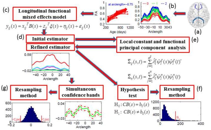
The aim of this paper is to present a functional analysis pipeline (FMEM) with several formal statistical inference tools for delineating the dynamic changes of fiber-tract statistics and their associations with a set of covariates obtained from longitudinal studies. A schematic overview of FMEM is given in Fig.1. Moreover, a short version of this paper has appeared in the conference proceedings of Information Processing in Medical Imaging (IPMI) 2013 (Yuan et al., 2013). Specifically, we propose a functional mixed effect model with two components: a varying-coefficient model for characterizing dynamic functional fixed effects between fiber-tract diffusion properties and some covariates and a set of functional random effects for capturing complex spatial-temporal correlation structure. Compared with the existing literature (Greven et al., 2010), there are three methodological contributions in this paper. The first one is to develop an efficient estimation method to spatially smooth varying coefficient functions, while accounting for spatial-temporal correlation structure. The second one is to propose a test procedure with both local and global test statistics for testing hypotheses of interest associated with functional responses. The third one is to approximate a simultaneous confidence band for quantifying the uncertainty in the estimated coefficient functions. FMEM provides a rigorous analytical tool for characterizing the dynamic changes of functional response data and their associations with a set of covariates. Using simulation procedures that mimic the real imaging data, we evaluate the finite sample performance of FMEM and demonstrate that FMEM significantly outperforms the standard point-wise mixed effects modeling approach.

Fig. 1.

A schematic overview of FMEM: a functional mixed effects model (c) for the repeatedly measured diffusion properties along a tract (a)-(b), a two-stage local linear regression method for estimating the coefficient functions (d), local constant estimators for covariance matrices adjusted by using a functional principal component analysis method (e), a hypothesis test for coefficient functions using global test statistics along with a resampling method for approximating the p-value of the global test statistics (f), and a method for constructing the confidence bands for the coefficient functions based on a resampling method (g).

2. Method

To compare diffusion properties in populations of DTIs, we use DTI atlas building with a group-wise longitudinal large deformation diffeomorphic registration method followed by atlas fiber tractography and fiber parametrization as described in Geng et al. (2012) to extract DTI fibers and establish DTI fiber correspondence across all DTI datasets from different subjects at all time points. Since this method has been described in Geng et al. (2012), we do not include a detailed description here for the sake of simplicity. Method section consists of data structure in subsection 2.1, method comparisons in subsection 2.3, and all components of FMEM in other subsections. Specifically, FMEM includes model formulation in subsection 2.2, initial estimator of varying coefficient functions in subsection 2.4, estimation of covariance operators in subsection 2.5, refined estimator of varying coefficient functions in subsection 2.6, smoothing individual functions in subsection 2.7, hypothesis testing in subsection 2.8, and constructing simultaneous confidence bands in subsection 2.9.

2.1. Data Structure

In a typical longitudinal DTI study, we observe diffusion properties (e.g., FA, or RD) along fiber bundles and some clinical/demographic variables measured at multiple time points from n subjects to investigate the white matter maturation and the association of white matter connectivity pattern with clinical/demographic variables of interest. We define r_i as the total number of time points, which can vary with the subject i, x_ij as a p_x × 1 vector of covariates of interest, such as age and gender, and t_ij as the j–th time point for the i–th subject for j = 1, ⋯, r_i and i = 1,…, n. We assume that at least some subjects i have at least 2 times points. Let s ∈ [0, L] be the arc length of any point on a specific fiber bundle relative to a fixed end point of the fiber bundle, where L is the longest arc length on the fiber bundle. For each subject i, let y_ij(s_m) be a specific diffusion property measured at the m–th grid point s_m ∈ [0, L] for m = 1,…, M at the j–th time point. Following spatial normalization, it is typical that y_ij(s_m) are measured at the same set of grid points for all subjects and all time points. This data structure is similar to that of standard longitudinal data, except that instead of observing scalar responses, y_ij, one observes curves or functions of location s, y_ij(s), multiple times for subject i. Thus, y_ij(s) exhibit the within-curve (spatial) correlations besides temporal correlations like in the standard longitudinal data. Note that when all subjects have only one time point, that is r_i = 1, y_ij(s) (can be reduced as y_i(s)) exhibit only the within-curve (spatial) correlations.

2.2. Functional Mixed Effects Model

A functional mixed effects model is defined as

$$y_{ij}\left(s\right)={\mathbf{x}}_{ij}^{T}B\left(s\right)+{\mathbf{z}}_{ij}^T{\xi }_i\left(s\right)+{\eta }_{ij}\left(s\right)+{∊}_{ij}\left(s\right),$$ (1)

where ξ_i(s) is a vector of functional random effects for subject i, z_ij is a p_z × 1 vector of covariates associated with ξ_i(s) and is commonly a subset of x_ij, ∊_ij(s) is a measurement error, and B(s) = (β₁(s),…, β_px(s))^T is a p_x × 1 vector of functional fixed effects. Model (1) includes two components: (i) a functional fixed-effect component ${\mathbf{x}}_{ij}^{T}B\left(s\right)$ for characterizing dynamic functional fixed effects between fiber-tract diffusion properties and some co-variates and (ii) a functional random-effect component ${\mathbf{z}}_{ij}^T{\xi }_i\left(s\right)+{\eta }_{ij}\left(s\right)$ for capturing complex spatial-temporal correlation structure. These two components play a critical role in making a formal statistical inference on B(s).

In model (1), η_ij(s) primarily characterizes within-curve spatial correlation structure, whereas ξ_i(s) primarily characterizes the subject-level variations and within-subject spatial-temporal correlation. Moreover, ξ_i(s), η_i(s), and ∊_i(s) are independent and identical copies of SP(0, Σ_ξ(s, s′)), SP(0, Σ_η(s, s′)I_ri), and SP(0, σ_∊(s)²1(s = s′)), respectively, where I_ri is a r_i × r_i identity matrix, and SP(μ(s), Σ(s, s′)) denotes a stochastic process vector with mean function μ(s) and covariance function Σ(s, s′). The covariance structure of y_i(s) = (y_i1(s),…, y_iri(s))^T, denoted by Σ_y,i(s, s′), is characterized as follows:

$${\Sigma }_{y,i}(s,s^{\prime })=\left({\mathbf{z}}_{i{j}_1}^T{\Sigma }_{\xi }(s,s^{\prime }){\mathbf{z}}_{i{j}_2}\right)+[{\Sigma }_{\eta }(s,s^{\prime })+{\sigma }_{∊}{\left(s\right)}^{2}1(s=s^{\prime })]{\mathbf{I}}_{r_i},$$ (2)

where $\left({\mathbf{z}}_{i{j}_1}^T{\Sigma }_{\xi }(s,s^{\prime }){\mathbf{z}}_{i{j}_2}\right)$ is a r_i × r_i matrix with the (j₁, j₂)–th element being ${\mathbf{z}}_{i{j}_1}^T{\Sigma }_{\xi }(s,s^{\prime }){\mathbf{z}}_{i{j}_2}$.

As an illustration, we considered FA values along the genu or splenium of the corpus callosum (Fig. 3) of 137 subjects obtained from our neonatal study of normal brain and each subject has up to three repeated measures at three time points corresponding to neonate, 1 year, and 2 years old. We may consider a quadratic growth fixed-effect model and a linear growth randomeffect model, which are, respectively, given by

$$\begin{array}{cc}\hfill {\mathbf{x}}_{ij}^{T}B\left(s\right)& ={\beta }_1\left(s\right)+g_i{\beta }_2\left(s\right)+{\text{Age}}_{ij}{\beta }_3\left(s\right)+{\text{Age}}_{ij}^2{\beta }_4\left(s\right),\hfill \\ \hfill {\mathbf{z}}_{ij}^T{\xi }_i\left(s\right)& ={\xi }_{i,1}\left(s\right)+{\text{Age}}_{ij}{\xi }_{i,2}\left(s\right),\hfill \end{array}$$ (3)

where g_i represents gender and Age_ij represents age at the j-th time point. In this case, we have p_z = 2, p_x = 4, ξ_i(s) = (ξ_i,1(s), ξ_i,2(s))^T, z_ij = (1, Age_ij)^T, B(d) = (β₁(s),…, β₄(s))^T, and ${\mathbf{x}}_{ij}={(1,g_i,{\text{Age}}_{ij},{\text{Age}}_{ij}^2)}^T$. For instance, in model (3), for any s, s′, we have Σ_ξ(s, s′) = (σ_ξ,kk′(s, s′)), which is a 2 × 2 matrix, and

$${\mathbf{z}}_{i{j}_1}^T{\Sigma }_{\xi }(s,s^{\prime }){\mathbf{z}}_{i{j}_2}={\sigma }_{\xi ,11}(s,s^{\prime })+{\sigma }_{\xi ,12}(s,s^{\prime })[{\text{Age}}_{i{j}_1}+{\text{Age}}_{i{j}_2}]+{\sigma }_{\xi ,22}(s,s^{\prime }){\text{Age}}_{i{j}_1}{\text{Age}}_{i{j}_2}.$$

Thus, model (1) can capture spatial-temporal correlation through ${\mathbf{z}}_{i{j}_1}^T{\Sigma }_{\xi }(s,s^{\prime }){\mathbf{z}}_{i{j}_2}$.

Fig. 3.

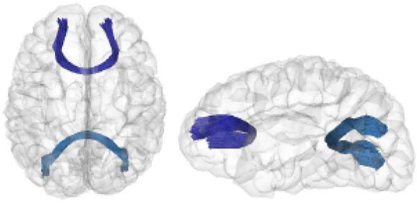
3D visualization of the genu and splenium of the corpus callosum in axial (left panel) and sagittal (right panel) views.

2.3. Comparisons with Existing Methods

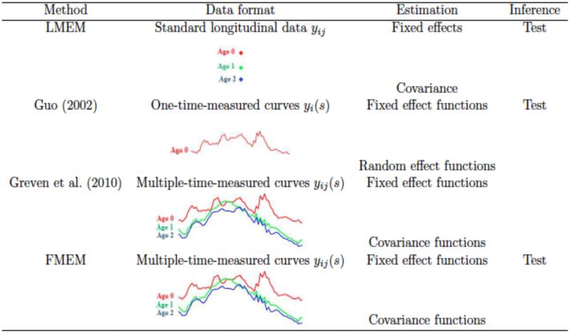
Model (1) is closely associated with several existing methods in the literature. Such methods include (i) standard linear mixed effects models (LMEM), (ii) a functional mixed effects models proposed in Guo (2002), and (iii) a longitudinal functional principal component analysis proposed in Greven et al. (2010). At each fixed s, model (1) reduces to LMEM. Fitting point-wise LMEM to longitudinal functional data ignores the spatial correlations that may exist in functional responses. We will show in Section 3 that FMEM outperforms LMEM under the presence of spatial correlations. When r_i = 1 for all i, model (1) reduces to the functional mixed effects model considered in Guo (2002). Fitting FMEM in Guo (2002) to longitudinal functional data ignores within-subject temporal correlations that may exist in longitudinal functional responses. Model (1) is essentially the same as that in Greven et al. (2010), which is the first statistical method for the analysis of repeatedly-measured functions. In Greven et al. (2010), the authors proposed an estimation procedure for fixed effect curves and spatial-temporal covariances, but no formal statistical inference tools, such as test statistics, were developed. In this paper, we present a longitudinal functional analysis pipeline, called FMEM, with several formal statistical inference tools for delineating the dynamic changes of diffusion properties along major white matter fiber bundles and their associations with a set of covariates of interest, such as age. Comparisons between FMEM and other three methods (i)-(iii) are displayed in Fig. 2 in terms of their applicability for data, estimation and inference tools. In the following subsections, We give a brief description of each component of FMEM.

Fig. 2.

Comparisons among linear mixed effects models (LMEM), Guo (2002)’s FMEM, Greven et al. (2010)’s longitudinal functional principal component model (LFPCA), and FMEM.

2.4. Initial Estimator of Varying Coefficient Functions

We use the local linear regression method and the weighted least squares estimation to estimate B(s) (Fan and Gijbels, 1992; Wand and Jones, 1995). Since the local linear regression method adapts automatically at the boundary points (Fan and Gijbels, 1992), it is ideal for dealing with scalar diffusion properties along fiber tracts with two ends, such as the genu and the splenium of the corpus callosum (see Fig. 3). Specifically, for a specific bandwidth h, we estimate B(s) by minimizing the following weighted least squares function

$$\sum _{i=1}^n\sum _{j=1}^{r_i}\sum _{m=1}^M{\{y_{ij}\left(s_m\right)-{\mathbf{x}}_{ij}^T[B\left(s\right)+\stackrel{.}{B}\left(s\right)(s_m-s)]\}}^2{K}_{h_1}(s_m-s),$$ (4)

where K(s) is a kernel function and K_h(s) = h⁻¹ K(s/h). The optimal estimator of B(s), denoted by B̂(s), is obtained at the optimal bandwidth selected by using a leave-one-curve-out cross-validation method (Zhang and Chen, 2007; Zhu et al., 2012). In practice, we standardize all covariates and diffusion properties to have mean zero and standard deviation one and then choose a common bandwidth for all covariates, which greatly increases computational efficiency in bandwidth selection. Note that we have not incorporated the temporal correlation in Equation (4), but we will address this issue in Section 2.6.

2.5. Estimating Covariance Operators

The covariance operator of y_ij(s) plays a crucial role in our proposed inference procedure. We propose an estimation procedure to estimate the covariance operator of y_ij(s) as follows:

• (i)We use the local constant method to estimate Σ_ξ(s, s′) and Σ_η(s, s′), denoted by ${\tilde{\Sigma }}_{\xi }(s,s^{\prime })$ and ${\tilde{\Sigma }}_{\eta }(s,s^{\prime })$, for each pair s ≤ s′ (Fan and Gijbels, 1992; Wand and Jones, 1995; Ramsay and Silverman, 2005; Welsh and Yee, 2006).
• (ii)We use the local constant method to smooth ${\tilde{\Sigma }}_{\xi }(s,s^{\prime })$ and ${\tilde{\Sigma }}_{\eta }(s,s^{\prime })$. It yields new estimates of Σ_ξ(s, s′) and Σ_η(s, s′), denoted by ${\widehat{\Sigma }}_{\xi }(s,s^{\prime })$ and ${\widehat{\Sigma }}_{\eta }(s,s^{\prime })$, respectively, for any s and s′.
• (iii)We use ${\widehat{\sigma }}_{∊}{\left(s\right)}^2=\{{\tilde{\Sigma }}_{\eta }(s,s)-{\widehat{\Sigma }}_{\eta }(s,s)\}1({\tilde{\Sigma }}_{\eta }(s,s)>{\widehat{\Sigma }}_{\eta }(s,s))$ to estimate σ_∊(s)², where 1(·) is an indicator function.

There is a practical issue associated with the above procedure. That is, the estimated ${\widehat{\Sigma }}_{\xi }(s,s^{\prime })$ and ${\widehat{\Sigma }}_{\eta }(s,s^{\prime })$ may not be semipositive definite. We employ an adjustment procedure proposed by Hall et al. (2008) to transform the estimated ${\widehat{\Sigma }}_{\xi }(s,s^{\prime })$ and ${\widehat{\Sigma }}_{\eta }(s,s^{\prime })$ into semipositive definite covariance operators. The key idea is to approximate the covariance operators by truncating the eigenfunctions associated with negative eigenvalues in the spectral representations of ${\widehat{\Sigma }}_{\xi }(s,s^{\prime })$ and ${\widehat{\Sigma }}_{\eta }(s,s^{\prime })$ (see Appendix A for details). Subsequently, we can substitute these estimators into (2) to obtain an estimate of Σ_y,i(s, s′), denoted by ${\widehat{\Sigma }}_{y,i}(s,s^{\prime })$.

2.6. Refined Estimator of Varying Coefficient Functions

In the initial estimation of varying coefficient functions, we ignore temporal correlation among repeated fiber-tract diffusion properties. To explicitly incorporate the temporal correlation, we refine the estimate of B(·) by incorporating the estimated covariance operators. Let X_i = [x_i1 ⋯ x_iri] be a p_x × r_i matrix. We reestimate A(s) by minimizing the following weighted least squares function:

$$\sum _{i=1}^n\sum _{m=1}^M{\left\{{[{\mathbf{y}}_i\left(s_m\right)-{\mathbf{X}}_i^T(B\left(s\right)+\stackrel{.}{B}\left(s\right)(s_m-s))]}^T{\widehat{\Sigma }}_{y,i}^{\left(1\right)}{(s_m,s_m)}^{-1∕2}\right\}}^{\otimes 2}{K}_{h_2}(s_m-s),$$ (5)

where ${\widehat{\Sigma }}_{y,i}^{\left(1\right)}(s,s^{\prime })={\widehat{\Sigma }}_{y,i}(s,s^{\prime })-{\widehat{\sigma }}_{∊}{\left(s\right)}^2{\mathbf{I}}_{r_i}1(s=s^{\prime })$. The objective function (5) includes both the spatial smoothness by using K_h2 (s_m − s) and the spatial-temporal correlation by using ${\widehat{\Sigma }}_{y,i}^{\left(1\right)}(s_m,s_m)$. We also select the bandwidth h₂ by using a leave-one-out cross validation criterion.

2.7. Smoothing Individual Functions

Let $g_{ij}\left(s\right)={\mathbf{z}}_{ij}^T{\xi }_i\left(s\right)+{\eta }_{ij}\left(s\right)$ for all i, j. Under certain smoothness conditions on η_ij(s) and ξ_i(s), we also employ the local linear regression technique to estimate all individual functions g_ij(s). The optimal estimator, denoted by ĝ_ij(s), is obtained at the optimal bandwidth selected by using the leave-one-out generalized cross-validation method.

2.8. Hypothesis Test

In longitudinal DTI studies, most scientific questions focus on the detection of dynamic changes of fiber tract diffusion properties along fiber bundles and the effects of covariates on diffusion properties. Such questions can often be formulated as linear hypotheses of B(s) as follows:

$$H_0:CB\left(s\right)={\mathbf{b}}_0\left(s\right)\text{for}\text{all}s\text{vs.}{H}_1:CB\left(s\right)\ne {\mathbf{b}}_0\left(s\right)\text{for}\text{some}s,$$ (6)

where C is a p_c × p_x matrix of full row rank and b₀(s) is a given p_c × 1 vector of functions.

As an illustration, in model (3), we may be interested in assessing the overall changes of FA’s along the fiber bundle from neonate to 2 years old. Statistically, for model (3), the hypothesis can be formulated as follows:

$$H_0:{\beta }_3\left(s\right)={\beta }_4\left(s\right)=0\text{for}\text{all}s\text{vs.}{H}_1:{\beta }_3{\left(s\right)}^2+{\beta }_4{\left(s\right)}^2\ne 0\text{for}\text{some}s.$$

In this case, we have

$$C=\left(\begin{array}{cccc}\hfill 0\hfill & \hfill 0\hfill & \hfill 1\hfill & \hfill 0\hfill \\ \hfill 0\hfill & \hfill 0\hfill & \hfill 0\hfill & \hfill 1\hfill \end{array}\right)\text{and}{\mathbf{b}}_0\left(s\right)\equiv \left(\begin{array}{c}\hfill 0\hfill \\ \hfill 0\hfill \end{array}\right)\text{for}\text{all}s.$$

We test the above null hypothesis by proposing a global test statistic S_n, defined by

$$S_n={\int }_0^L{S}_n\left(s\right)ds,$$ (7)

where S_n(s) is a local test statistic defined by

$$S_n\left(s\right)=\mathbf{d}{\left(s\right)}^T{\left\{C{\left[\sum _{i=1}^n{\mathbf{X}}_i{\widehat{\Sigma }}_{y,i}^{\left(1\right)}{(s,s)}^{-1}{\mathbf{X}}_i^T\right]}^{-1}{C}^T\right\}}^{-1}\mathbf{d}\left(s\right),$$ (8)

in which d(s) = Cvec(B̂(s) − bias(B̂(s))) − b₀(s). The asymptotic distribution of S_n is very complicated and it is difficult to directly approximate the percentiles of S_n under the null hypothesis. Instead, we propose to use a novel wild bootstrap method described in Appendix B to obtain the critical values of S_n and approximate the p-value of S_n. The key challenge of this wild bootstrap method is to preserve the spatial-temporal correlation in model (1).

2.9. Simultaneous confidence bands

For a given significance level α, we construct a simultaneous confidence band for each β_l(s) such that

$$P({\widehat{\beta }}_l^{L,\alpha }\left(s\right)<{\beta }_l\left(s\right)<{\widehat{\beta }}_l^{U,\alpha }\left(s\right)\text{for}\text{all}s\in [0,L])=1-\alpha ,$$ (9)

where ${\beta }_l^{L,\alpha }\left(s\right)$ and ${\beta }_l^{U,\alpha }\left(s\right)$ are, respectively, the lower and upper limits of the confidence band. Specifically, a 1 − α simultaneous confidence band for β_l(s) is given as follows:

$$\left({\widehat{\beta }}_l\left(s\right)-\mathrm{bias}\left({\widehat{\beta }}_l\left(s\right)\right)-\frac{C_l\left(\alpha \right)}{\sqrt{n}},{\widehat{\beta }}_l\left(s\right)-\mathrm{bias}\left({\widehat{\beta }}_l\left(s\right)\right)+\frac{C_l\left(\alpha \right)}{\sqrt{n}}\right),$$ (10)

where C_l(α) is a scalar. Since the calculation of ${\widehat{\beta }}_l\left(s\right)$ has been discussed and the effect of dropping $\mathrm{bias}\left({\widehat{\beta }}_l\left(s\right)\right)$ is negligible, the critical issue is to determine C_l(α). We develop a novel efficient resampling method described in Appendix C to approximate C_l(α). The key challenge of this resampling method is to preserve the spatial-temporal correlation in model (1).

3. Simulation Studies and A Real Example

In this section, we use Monte Carlo simulations and a real example to evaluate the finite-sample performance of FMEM and compare FMEM with LMEM. All computations for these numerical examples were done in Matlab on an IBM ThinkCentre M50 workstation. The computation for FMEM is relatively efficient for moderate and even large data. The computational time for FMEM can be further reduced by using other computer languages, such as C++.

3.1. Simulation Studies

We conducted a Monte Carlo simulation study to evaluate the Type I and II error rates of the global test statistic S_n. We simulated FA values along the genu of the corpus callosum tract (Fig. 3) according to model (1), in which we set

$${\xi }_i\left(s_m\right)=\sum _{k=1}^{\infty }{\zeta }_{ik}^{\xi }{\psi }_k^{\xi }\left(s_m\right)\text{and}{\eta }_{ij}\left(s_m\right)=\sum _{k=1}^{\infty }{\zeta }_{ijk}^{\eta }{\psi }_k^n\left(s_m\right),$$ (11)

where ${\zeta }_{ik}^{\xi }$ and ${\zeta }_{ijk}^{\eta }$ were independently generated from $N(0,{\lambda }_k^{\xi })$ and $N(0,{\lambda }_k^{\eta })$ for all i, j, and k. Specifically, we set the parameters according to our real imaging data as follows: n = 137, M = 64, r_i = 1, 2 (or 3), x_ij = (1, Dir_ij, G_i, Age_ij)^T, B(s) = (β₁(s), β₂(s), β₃(s), β₄(s))^T, and z_ij = (1, Age_ij)^T for i = 1, ⋯, 137, where Dir_ij, G_i and Age_ij, respectively, denote the indicator of different number of gradient directions used, gender, and the gestational age at the j–th scan time of the i–th subject. To mimic real imaging data, we applied model (1) to FA measures along the genu of the corpus callosum tract from all 137 infants in our clinical data to estimate B(s) by B̂(s), ${\psi }_k^{\xi }\left(s\right)$ by ${\widehat{\psi }}_k^{\xi }\left(s\right)$, ${\psi }_k^{\eta }\left(s\right)$ by ${\widehat{\psi }}_k^{\eta }\left(s\right)$, ${\lambda }_k^{\xi }$ by ${\widehat{\lambda }}_k^{\xi }$, and ${\lambda }_k^{\eta }$ by ${\widehat{\lambda }}_k^{\eta }$,. The curves of the varying coefficient functions of B̂(s) are presented in Fig. 5. According to the results in Section 3.2, the age effect is significant for our clinical data. So we fixed all parameters in model (1) at their corresponding estimated parameters, whereas β₄(s) was set as $c{\widehat{\beta }}_4\left(s\right)$, where c is set at different values in order to study the Type I and II error rates of our global test statistic in testing the age effect.

Fig. 5.

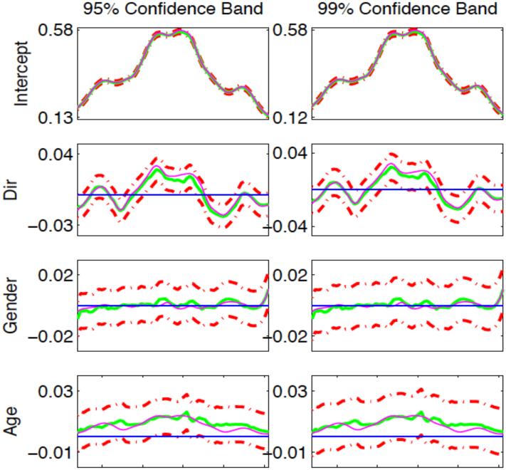
Simulation study: Typical 95% (left) and 99% (right) simultaneous confidence bands for varying coefficient functions β_l(s). The magenta, green solid, and red dash-dotted curves are, respectively, the true curves, the estimated varying coefficient functions and their 95% and 99% confidence bands. The blue solid horizontal line is the line crossing the origin.

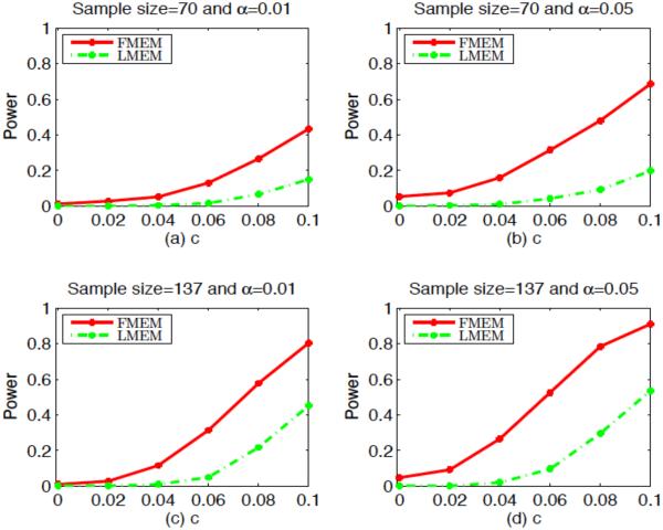
We have three aims in this simulation study. The first aim is to evaluate the Type I and II error rates of the global test statistic S_n. In neuroimaging studies, some scientific questions require the assessment of the development of white matter across age. We formulated the questions as testing the null hypothesis H₀ : β₄(s) = 0 for all s along the genu against H₁ : β₄(s) ≠ 0 for at least one s on the tract. We first fixed c = 0 to assess the Type I error rates for S_n, and then we set c = 0.02, 0.04, 0.06, 0.08, and 0.1 to examine the Type II error rates for S_n at different effect sizes. In order to evaluate the Type I and II error rates at different sample sizes, we let n = 137 and 70. For n = 137, the values of indicator of number of gradient directions, gender and age were set the same as the 137 subjects in our clinical study. For n = 70, we randomly chose 35 males and 35 females from the 137 subjects and used their values for indicator of number of gradient directions, gender and age to simulate the values of FA along the genu tract. We applied the estimation procedure of FMEM to the simulated FA measures along the genu. We approximated the p-value of S_n by using the wild bootstrap method with G = 500. For each c, we set the significance level α at both 0.05 and 0.01 and used 500 replications to estimate the rejection rate of S_n. At a fixed α, if the Type I rejection rate is smaller than α, then the test is conservative, whereas if the Type I rejection rate is greater than α, then the test is anticonservative, or liberal. Fig. 4 presents the rejection rates of S_n across all effect sizes at the two significance levels (α = 0.05 or 0.01). It is observed that Type I error rates are well maintained with the values 0.048 and 0.01, respectively, at the two significance levels. In addition, the statistical power for rejecting the null hypothesis increases with the sample size, the effect size and the significance level, which is consistent with our expectation. The Monte Carlo error rate is $\sqrt{\alpha (1-\alpha )∕N}=0.0097$ with N = 500.

Fig. 4.

Simulation study: Type I and Type II error rates as functions of c. Rejection rates of S_n based on the wild bootstrap method are calculated at six different values of the effect size c for sample size 70 and 137 at the 0.01 and 0.05 significance levels using FMEM and LMEM.

The second aim is to show that FMEM outperforms standard LMEM. To this end, we first fitted linear mixed effects model at each s_m without separating η_ij(s_m) from ∊_ij(s_m). Then, we calculated the global testing statistic except that we replaced ${\Sigma }_{y,i}^{\left(1\right)}(s_m,s_m)$ in S_n with ${\Sigma }_{y,i}^{\left(2\right)}(s_m,s_m)={\mathbf{z}}_{ij}^T{\Sigma }_{\xi }(s_m,s_m){\mathbf{z}}_{ij}+{\sigma }_{∊}^2\left(s_m\right)$. Finally, we calculated the p-values with the wild bootstrap method as in FMEM. Table 1 shows that LMEM is much less powerful than FMEM (also see Fig. 4).

Table 1.

Simulation study: the Type I and Type II error rates of S_n under LMEM and FMEM.

c	sample size = 70				sample size = 137
	α = 0.01		α = 0.05		α = 0.01		α = 0.05
	LMEM	FMEM	LMEM	FMEM	LMEM	FMEM	LMEM	FMEM
0	0.000	0.012	0.000	0.054	0.002	0.010	0.002	0.048
0.02	0.000	0.028	0.004	0.074	0.002	0.028	0.002	0.092
0.04	0.004	0.052	0.010	0.160	0.010	0.116	0.020	0.266
0.06	0.016	0.130	0.042	0.314	0.050	0.314	0.096	0.526
0.08	0.066	0.266	0.092	0.480	0.218	0.578	0.296	0.784
0.1	0.150	0.434	0.198	0.6860	0.452	0.804	0.536	0.910

The third aim is to examine the coverage probabilities of the simultaneous confidence bands for all varying coefficient functions β_l(s) for l = 1, 2, 3, 4 in B(s). We only considered the simulated FA measures at c = 0.1 and constructed the 95% and 99% simultaneous confidence bands for all β_l(s). Table 2 summarizes the empirical coverage probabilities based on 500 replications for α = 0.01 and 0.05. The coverage probabilities are quite close to the prespecified confidence levels. Fig. 5 presents typical 95% and 99% simultaneous confidence bands for coefficient functions β_l(s). The simultaneous confidence bands contain the horizontal line crossing (0, 0) for the gender effect whereas the horizontal line is out of the 95% and 99% simultaneous confidence band for number of directions and age effects, which indicates the significant number of directions and age effects at the significance levels α = 0.05 and 0.01. This is consistent with our simulation setup and our findings in the real data analysis that age and number of directions significantly influence the FA measures.

Table 2.

Simulated coverage probabilities for varying coefficient functions in B(x) = (β_l(x)) based on 500 replications at the significance levels α = 0.01 and 0.05.

c	α = 0.05				α = 0.01
	intercept	Dir	Gender	Age	intercept	Dir	Gender	Age
	l = 1	l = 2	l = 3	l = 4	l = 1	l = 2	l = 3	l = 4
0.1	0.942	0.930	0.946	0.946	0.992	0.986	0.986	0.980

3.2. A Real Example

This study was approved by the Institutional Review Board of the University of North Carolina (UNC) School of Medicine. Children analyzed in this work were taken from the control group of a longitudinal study to investigate neonatal brain development in children at high risk for neurodevelopmental disorders. After applying a certain exclusion criteria, 298 high quality scans are available for 137 children (83 males and 54 females). Demographic information and distribution of scan availability are shown in Tables 3 and 4.

Table 3.

Demographic characteristics for participants.

Gender: Male/Female	83/54
Gestational age at birth (weeks)	38.67 ± 1.74
Age at scan 1(days)	297.89 ± 13.90
Age at scan 2 (days)	655.34 ± 24.00
Age at scan 3 (days)	1021.70 ± 28.26
Number of Gradient directions
dir6/dir42 at scan 1	80/24
dir6/dir42 at scan 2	59/44
dir6/dir42 at scan 3	42/49

Table 4.

Distributions of scan availability.

Available scans	N
Neonate scan only	1
1 year scan only	2
2 year scan only	3
Neonate + 1 year scan	43
Neonate + 2 year scan	30
1 year + 2 year scan	28
Neonate + 1 year + 2 year scan	30

A 3 T Allegra head-only MR system (Siemens Medical Solutions, Erlangen, Germany) was used to acquire all the images. The system was equipped with a maximal gradient strength of 40 mT/m and a maximal slew rate of 400 mT/(m · ms). The DTI images were obtained by using a single shot EPI DTI sequence with the following variables: TR/TE= 5200/73 ms, slice thickness= 2 mm, in-plane resolution= 2 × 2 mm² with eddy current compensation. We applied the 6 or 42 non-collinear directions at the b-value of 1000 s/mm² with a reference scan (b = 0). When the sequence with 6 gradient directions was applied, to improve the signal-to-noise ratio of the images, a total of five scans were acquired and averaged.

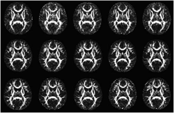
A weighted least squares estimation method were used to estimate diffusion tensors (Zhu et al., 2007; Basser et al., 1994). A DTI atlas building with a group-wise longitudinal large deformation diffeomorphic registration method followed by atlas fiber tractography and fiber parametrization as described in (Joshi et al., 2004; Geng et al., 2012) were used to extract DTI fibers and establish DTI fiber correspondence across all DTI datasets from different subjects at all time points (see Fig. 6 for the visualization of the atlas building). The fiber tractography was done by using the freely available ‘FiberTracking’ software (http://www.ia.unc.edu)/dev). While several DTI fiber tracts were tracked, we chose to focus in this paper on the commissural bundles of the genu and splenium of the corpus callosum (see Fig. 3) to illustrate the applicability of our method to assessing the effects of covariates of interest, such as age, gender, and number of gradient directions, in this study. Three diffusion properties including FA, RD, and AD, were extracted at each grid point along the selected fiber tracts for all 137 infants.

Fig. 6.

2D axial views of 15 deformed images (FA of the deformed tensor images after registration). The first, second and third rows include 5 images randomly selected from neonate, 1- year-old and 2-year-old data, separately.

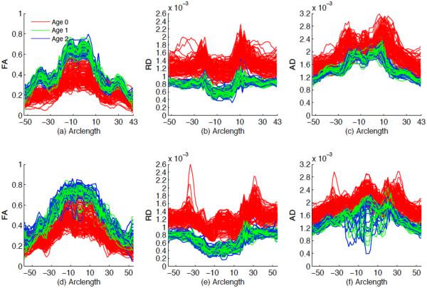
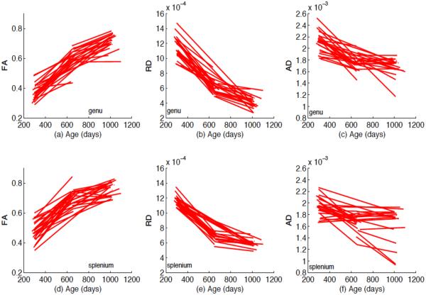
For the two selected tracts, we fitted the functional mixed effects model (1) to the FA, RD and AD values from all 137 subjects, in which x = (1, Dir, G, Age₁, Age₂)^T, z = (1, Age₁, Age₂)^T and Age₁ (or Age₂) is an indicator variable indicating whether a subject belongs to the first (or second) year age group. The coefficient functions related to Age₁ and Age₂ can be used to investigate whether there are some diffusion changes from neonate to the first year of life, from the first year to the second year and from neonate to the second year at each grid point, the direction of changes and the changing speed (indicating white matter maturation speed). The positive value indicates the increasing trend. In addition, it is observed from Fig. 7 that there are random subject-to-subject variations in FA, RD and AD measures at each grid point along the two tracts. Fig. 8 also shows that there are random subject-to-subject variations in the age effect on FA, RD and AD measures at the selected location. To take care of these inter-subject variations, random intercept and age effects were included in the model. Then we estimated the functional coefficients B(s) and constructed their 95% simultaneous confidence bands to look at the uncertainty in the estimated coefficient functions. We also constructed the global test statistic S_n via Equation (7) to test for the significance of gender, number of gradient directions and age effects on FA, RD and AD values. We approximated the p-value of S_n using the resampling method with G = 5, 000 replications.

Fig. 7.

FA, RD and AD values along the genu ((a), (b) and (c)) and splenium ((d), (e) and (f)) of the corpus callosum for all 137 subjects in each age group.

Fig. 8.

FA, RD and AD values varying over age at a selected location (arclength=−8.75 or arclength=−14.07) along the genu ((a), (b) and (c)) and splenium ((d), (e) and (f)) of the corpus callosum for the selected 35 subjects.

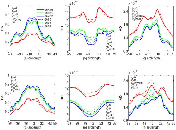
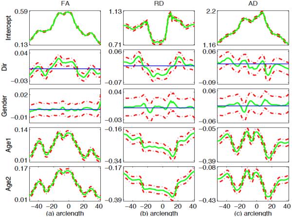
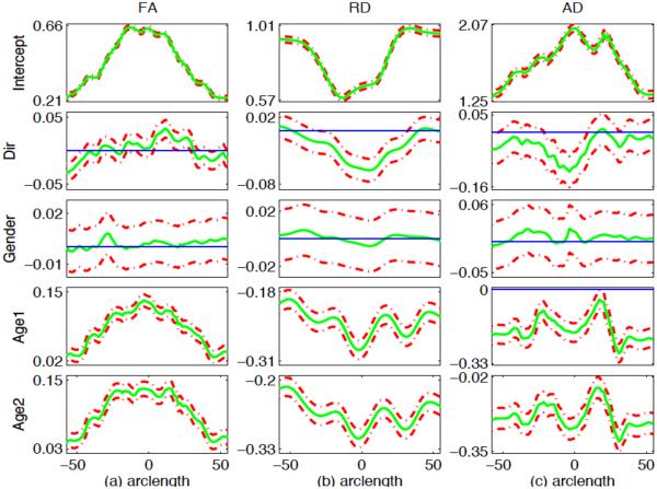
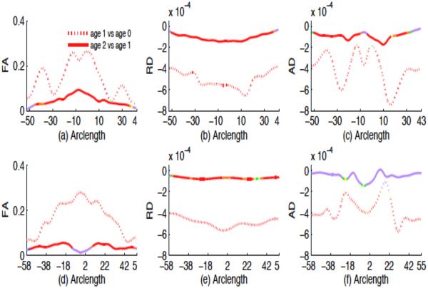
The hypothesis testing results show that there are significant age and number of gradient directions effects on FA, RD and AD values but gender was not found to be significant for these two corpus callosum tracts (see Fig. 9), which agrees with the findings in panels (a)-(c) of Figures 10 and 11. The FA, RD and AD values are significantly different between neonate versus the first year, and between the first year versus the second year with p value < .0001, far smaller than 0.05 significance level. In general, FA increases while RD and AD decrease from neonate to the first year and then from the first year to the second year, even across all locations of the two tracts (see Fig. 12). Also changes of all three diffusion indices in the first year are larger than in the second year (see Figures 9 and 12). This might reflect that white matter development is not uniformly across time. It is observed from Fig. 10 that when 6-gradient-directions instead of 42-gradient-directions was used, central regions of the genu of the corpus callosum show significantly smaller FA values and larger RD values while the peripheral regions show significantly larger FA and smaller RD values. For the splenium of the corpus callosum, central regions show significantly smaller FA values and larger RD and AD values, when 6-gradient-directions instead of 42-gradient-directions was used (see Fig. 11). This reflects different regional impact of low number of gradient directions on diffusion properties along these two callosal tracts. Essentially, it may inflate FA values and deflate RD and AD values in the peripheral regions and vice versus for the central regions.

Fig. 9.

Mean FA, RD and AD values along the genu ((a), (b) and (c)) and splenium ((d), (e) and (f)) of the corpus callosum tract and gender, number of gradient directions and age effects on FA, RD and AD values. Solid lines are mean FA, RD and AD curves for the 42 gradient directions while the dashed lines are mean curves for the 6 gradient directions. Red for neonate, green for the first year age, and blue for the second year age. p₁ is the p value for the difference in the diffusion measure between neonate and the first year, p₂ is the p value for the difference in the diffusion measure between neonate and the second year, p₁₂ is the p value for the difference between the first year and the second year, p_G is the p value for the gender effect, p_Dir is the p value for the effect of the number of gradient directions.

Fig. 10.

95% simultaneous confidence bands for varying coefficient functions for FA (a), RD (b) and AD (c) along the genu of the corpus callosum tract. The solid curves are the estimated coefficient functions, and the dashed curves are the 95% confidence bands. The thin horizontal line is the line crossing the origin.

Fig. 11.

95% simultaneous confidence bands for varying coefficient functions for FA (a), RD (b) and AD (c) along the splenium of the corpus callosum tract. The solid curves are the estimated coefficient functions, and the dashed curves are the 95% confidence bands. The thin horizontal line is the line crossing the origin.

Fig. 12.

Mean changes in FA, RD and AD along the genu (a)-(c) and splenium (d)-(f) of the corpus callosum tract. Colors indicate different p values with red (p value < 0.01), orange (0.01 ≤ p value < 0.02), yellow (0.02 ≤ p value < 0.03), green (0.03 ≤ p value < 0.04), and blue (0.04 ≤ p value < 0.05) and light purple (p value ≤ 0.05).

4. Discussion

We have developed a FMEM pipeline for the spatial and temporal analysis of longitudinal fiber tract diffusion properties. Our functional mixed effect model include the functional fixed-effect component and the functional random-effect component for the explicit incorporation of spatial smoothness and spatial-temporal correlation. These two components are critical for correctly making formal statistical inferences on longitudinal functional responses. We have explicitly incorporated these two components in both estimation and testing procedures. We have used simulations to demonstrate that FMEM outperforms standard mixed effects model coupled with a multiple comparison method.

We have demonstrated the applicability of FMEM by applying it to the analysis of dynamic changes of diffusion properties along two corpus callosum tracts in a clinical study of neurodevelopment. In agreement with previous studies (Neil et al., 1998; Gao et al., 2009; Geng et al., 2012), increased FA and decreased AD and RD were detected across almost all locations of the splenium and genu of the corpus callosum tracts in the first two years of life. Our results showed that the changes in diffusion properties are greater in the first year than in the second year. We have shown some strong number-of-diffusion-gradient-direction effect on diffusion properties along fiber tracts.

Several important issues need to be addressed in future research. Firstly, it is critically important to develop an unbiased image-processing framework for longitudinal neuroimaging analysis (Reuter and Fischl, 2011; Keihaninejad et al., 2013; Yushkevich et al., 2010; Hua et al., 2011). Secondly, the FMEM procedure is solely powerful for these major white matter tracts, in which one can establish the common localization across subjects. In practice, however, white matter tract pattern and structure may vary dramatically across subjects due to both registration error and population heterogeneity. For instance, in some heterogenous populations, it is possible that tract-specific changes occur in only a subset of subjects. Therefore, it is important and interesting to develop new analytical tools to quantitatively extract white matter tract pattern and structure for other DTI studies. Thirdly, although we focus on linear functions in both the functional fixed-effect component and the functional random-effect component, it is interesting to develop nonlinear functional mixed effects models, which are important for quantifying complex growth curves. Developing statistical methods for nonlinear functional mixed effects models faces up with many new challenges both computationally and theoretically. Fourthly, we will extend FMEM from simple longitudinal studies to more complex longitudinal twin/familial studies and extend FMEM to the analysis of whole-brain images as a single piecewisely smoothed function with possible jumps and edges.

• Develop a FMEM for adaptive analysis of longitudinal functional data.

• Useful for understanding the development of white matter fiber bundles.

• Characterize the development of white matter diffusivities

Appendix A: Approximating the covariance operators using the method proposed by Hall et al. (2008)

Let $\{({\widehat{\lambda }}_l^{\xi },{\widehat{\psi }}_l^{\xi }\left(s\right)):l=1,\dots ,\infty \}$ and $\{({\widehat{\lambda }}_l^{\eta },{\widehat{\psi }}_l^{\eta }\left(s\right)):l=1,\dots ,\infty \}$ be, respectively, the eigenvalue-eigenfunction pairs of ${\widehat{\Sigma }}_{\xi }(s,s^{\prime })$ and ${\widehat{\Sigma }}_{\eta }(s,s^{\prime })$ such ${\widehat{\lambda }}_1^{\xi }\ge {\widehat{\lambda }}_2^{\xi }\ge \cdots$ and ${\widehat{\lambda }}_1^{\eta }\ge {\widehat{\lambda }}_2^{\eta }\ge \cdots$. Then, the adjusted estimators of Σ_ξ(s, s′) and Σ_η(s, s′) are, respectively, given by

$${\check{\Sigma }}_{\xi }(s,s^{\prime })=\sum _{l=1}^{n_{\xi }}{\widehat{\lambda }}_l^{\xi }{\widehat{\psi }}_l^{\xi }\left(s\right){\widehat{\psi }}_l^{\xi }{\left(s^{\prime }\right)}^{T}1({\widehat{\lambda }}_l^{\xi }>0)$$ (12)

$${\check{\Sigma }}_{\eta }(s,s^{\prime })=\sum _{l=1}^{n_{\eta }}{\widehat{\lambda }}_l^{\eta }{\widehat{\psi }}_l^{\eta }\left(s\right){\widehat{\psi }}_l^{\eta }{\left(s^{\prime }\right)}^{T}1({\widehat{\lambda }}_l^{\eta }>0),$$ (13)

where n_ξ and n_η are positive integers such that the proportions of explained variance by eigenvalues exceed a pre-specific value, such as 0.90.

Appendix B: Wild Bootstrap Methods for Approximating the Null Distribution of S_n

The wild bootstrap consists of the following three steps:

Step 1. Fit model (1) under the null hypothesis H₀, which yields B̂*(s_m), ${\widehat{g}}_{ij}^{\ast }\left(s_m\right)$ and ${\widehat{∊}}_{ij}^{\ast }\left(s_m\right)=y_{ij}\left(s_m\right)-{\mathbf{x}}_{ij}^T{\widehat{B}}^{\ast }\left(s_m\right)-{\widehat{g}}_{ij}^{\ast }\left(s_m\right)$ for i = 1,…, n and m = 1,…, M.

Step 2. Generate a random sample ${\tau }_i^{\left(g\right)}$ and τ_ij(s_m)^(g) from a N(0,1) generator for i = 1, …, n and m = 1, …, M and then construct

$${\widehat{y}}_{ij}^{}{\left(s_m\right)}^{\left(g\right)}={\mathbf{x}}_{ij}^T{\widehat{B}}^{\ast }\left(s\right)+{\tau }_i^{\left(g\right)}{\widehat{g}}_{ij}^{\ast }\left(s_m\right)+{\tau }_{ij}{\left(s_m\right)}^{\left(g\right)}{\widehat{∊}}_{ij}^{\ast }\left(s_m\right).$$

Then, based on ŷ_ij(s_m)^(g), we recalculate B̂(s)^(g), bias(B̂(s)^(g)), and d(s)^(g) = Cvec(B̂(s)^(g) − bias(B̂(s)^(g))) − b₀(s). We also note that Cvec(B̂(s)^(g)) ≈ b₀ and Cvec(bias(B̂(s)^(g))) ≈ 0. Thus, we can drop the term bias(B̂(s)^(g)) in d(s)^(g) for computational efficiency. Subsequently, we compute

$$S_n^{\left(g\right)}=n{\int }_0^L\mathbf{d}{\left(s\right)}^{\left(g\right)T}{\left\{C{\left[\sum _{i=1}^n{\mathbf{X}}_i{\widehat{\Sigma }}_{y,i}^{\left(1\right)}{(s,s)}^{-1}{\mathbf{X}}_i^T\right]}^{-1}{C}^T\right\}}^{-1}\mathbf{d}{\left(s\right)}^{\left(g\right)}ds.$$

Step 3. Aggregate the results of Step 2 over g = 1, ⋯, G to obtain $\{S_n^{\left(g\right)}:g=1,\dots ,G\}$ and then calculate $p=G^{-1}{\sum }_{g=1}^{G}1(S_n^{\left(g\right)}\ge S_n)$. If p is smaller than a pre-specified significance level α, say 0.05, then one rejects the null hypothesis H₀.

Appendix C: Resampling Method for Approximating C_l(α)

The resampling bootstrap consists of the following three steps:

Step 1. We calculate ${\widehat{\mathbf{r}}}_i\left(s_m\right)={\mathbf{y}}_i\left(s_m\right)-{\mathbf{X}}_i^T\widehat{B}\left(s_m\right)$ for all i and m.

Step 2. For g = 1,…, G, we independently simulate $\{{\tau }_i^{\left(g\right)}:i=1,\dots ,n\}$ from N(0,1) and calculate a stochastic process G(s)^(g) given by

$$\sqrt{n}[I_p\otimes (1,0)]\mathrm{vec}\left(\Sigma {(h_2,s)}^{-1}\sum _{i=1}^n{\tau }_i^{\left(g\right)}\sum _{m=1}^M{K}_{h_2}(s_m-s)[{\mathbf{S}}_{h_2}(s_m-s)\otimes {\mathbf{X}}_i]{\widehat{\Sigma }}_{y,i}^{\left(1\right)}{(s_m,s_m)}^{-1}{\widehat{\mathbf{r}}}_i\left(s_m\right)\right),$$

where $\Sigma (s,h_2)={\sum }_{i=1}^n{\sum }_{j=1}^{r_i}{\sum }_{m=1}^M{K}_{h_2}(s_m-s)[{\mathbf{x}}_{ij}^{\otimes 2}\otimes {\mathbf{s}}_{h_2}{(s_m-s)}^{\otimes 2}]$

Step 3. We calculate sup_s∈[0,1] |e_lG(s)^(g)| for all g, where e_l be a p × 1 vector with the l-th element 1 and 0 otherwise, and use their 1 − α empirical percentile to estimate C_l(α).

References

- Agosta F, Henry R, Migliaccio R, Neuhaus J, Miller B, Dronkers N, Brambati S, Filippi M, Ogar J, Wilson S, Gorno-Tempini M. Language networks in semantic dementia. Brain. 2010;133:286–299. doi: 10.1093/brain/awp233. [DOI] [PMC free article] [PubMed] [Google Scholar]
- Basser PJ, Mattiello J, LeBihan D. Mr diffusion tensor spectroscopy and imaging. Biophysical Journal. 1994;66:259–267. doi: 10.1016/S0006-3495(94)80775-1. [DOI] [PMC free article] [PubMed] [Google Scholar]
- Budde M, Kim J, Liang H, Schmidt R, Russell J, Cross A, Song S. Toward accurate diagnosis of white matter pathology using diffusion tensor imaging. Magn Reson Med. 2007;57:688–695. doi: 10.1002/mrm.21200. [DOI] [PubMed] [Google Scholar]
- Cascio CJ, Gerig G, Piven J. Diffusion tensor imaging: Application to the study of the developing brain. J Am Acad Child Adolesc Psychiatry. 2007;46:213–223. doi: 10.1097/01.chi.0000246064.93200.e8. [DOI] [PubMed] [Google Scholar]
- Colby JB, Soderberg L, Lebel C, Dinov ID, Thompson PM, Sowell ER. Along-tract statistics allow for enhanced tractography analysis. NeuroImage. 2012;59:3227–3242. doi: 10.1016/j.neuroimage.2011.11.004. [DOI] [PMC free article] [PubMed] [Google Scholar]
- Diggle P, Heagerty P, Liang KY, Zeger S. Analysis of Longitudinal Data. 2nd Oxford University Press; New York: 2002. [Google Scholar]
- Ding X, Sun Y, Braass H, Illies T, Zeumer H, Lanfermann H, Fiehler J. Evidence of rapid ongoing brain development beyond 2 years of age detected by fiber tracking. American Journal of Neuroradiology. 2008;29:1261–1265. doi: 10.3174/ajnr.A1097. [DOI] [PMC free article] [PubMed] [Google Scholar]
- Evans AC, Group. BDC. The nih mri study of normal brain development. NeuroImage. 2006;30:184–202. doi: 10.1016/j.neuroimage.2005.09.068. [DOI] [PubMed] [Google Scholar]
- Fan J, Gijbels I. Variable bandwidth and local linear regression smoothers. Annals of Statistics. 1992;21:433–446. [Google Scholar]
- Fitzmaurice GM, Laird NM, Ware JH. Wiley; New York: 2004. Applied Longitudinal Analysis. [Google Scholar]
- Gao W, Lin W, Chen Y, Gerig G, Smith J, Jewells V, Gilmore J. Temporal and spatial development of axonal maturation and myelination of white matter in the developing brain. American Journal of Neuroradiology. 2009;30:290–296. doi: 10.3174/ajnr.A1363. [DOI] [PMC free article] [PubMed] [Google Scholar]
- Geng X, Gouttard S, Sharma A, Gu H, Styner M, Lin W, Gerig G, Gilmore JH. Quantitative tract-based white matter development from birth to age 2 years. NeuroImage. 2012;61:542–557. doi: 10.1016/j.neuroimage.2012.03.057. [DOI] [PMC free article] [PubMed] [Google Scholar]
- Gilmore J, Kang C, Evans D, Wolfe H, Smith J, Lieberman J, Lin W, Hamer R, Styner M, Gerig G. Diffusion tensor imaging of normal white matter maturation from late childhood to young adulthood: voxel-wise evaluation of mean diffusivity, fractional anisotropy, radial and axial diffusivities, and correlation with reading development. Am. J. Psychiatry. 2010;167:1083–1091. [Google Scholar]
- Goodlett CB, Fletcher PT, Gilmore JH, Gerig G. Group analysis of dti fiber tract statistics with application to neurodevelopment. NeuroImage. 2009;45:S133–S142. doi: 10.1016/j.neuroimage.2008.10.060. [DOI] [PMC free article] [PubMed] [Google Scholar]
- Greven S, Crainiceanu C, Caffo B, Reich D. Longitudinal functional principal component analysis. Electron. J. Statist. 2010;4:1022–1054. doi: 10.1214/10-EJS575. [DOI] [PMC free article] [PubMed] [Google Scholar]
- Guo W. Functional mixed effects models. Biometrics. 2002;58:121–128. doi: 10.1111/j.0006-341x.2002.00121.x. [DOI] [PubMed] [Google Scholar]
- Hall P, Muller H, Yao F. Modelling sparse generalized longitudinal observations with latent gaussian processes. J. R. Statist. Soc. B. 2008;70:703–723. [Google Scholar]
- Haynes R, Borenstein N, Desilva T, Folkerth R, Liu L, Volpe J, Kinney H. Axonal development in the cerebral white matter of the human fetus and infant. J Comp Neurol. 2005;484:156–167. doi: 10.1002/cne.20453. [DOI] [PubMed] [Google Scholar]
- Hua X, Gutman B, Boyle CP, Rajagopalan P, Leow AD, Yanovsky I, Kumar AR, Toga AW, Jack CR, Schuff N, Alexander GE, Chen K, Reiman EM, Weiner MW, Thompson PM, ADNI Accurate measurement of brain changes in longitudinal mri scans using tensor-based morphometry. NeuroImage. 2011;57:5–14. doi: 10.1016/j.neuroimage.2011.01.079. [DOI] [PMC free article] [PubMed] [Google Scholar]
- Huppi P, Dubois J. Diffusion tensor imaging of brain development. Semin. Fetal Neonatal Med. 2006;11:489–497. doi: 10.1016/j.siny.2006.07.006. [DOI] [PubMed] [Google Scholar]
- Joshi S, Davis B, Jomier M, Gerig G. Unbiased diffeomorphic atlas construction for computational anatomy. Neuroimage. 2004;23:S151–S160. doi: 10.1016/j.neuroimage.2004.07.068. [DOI] [PubMed] [Google Scholar]
- Keihaninejad S, Zhang H, Ryan NS, Malone IB, Modat M, Cardoso MJ, Cash DM, Fox NC, Ourselin S. An unbiased longitudinal analysis framework for tracking white matter changes using diffusion tensor imaging with application to alzheimer’s disease. NeuroImage. 2013;72:153–163. doi: 10.1016/j.neuroimage.2013.01.044. [DOI] [PubMed] [Google Scholar]
- Lebel C, Beaulieu C. Longitudinal development of human brain wiring continues from childhood into adulthood. The Journal of Neuroscience. 2011;31:10937–10947. doi: 10.1523/JNEUROSCI.5302-10.2011. [DOI] [PMC free article] [PubMed] [Google Scholar]
- McGraw P, Liang L, Provenzale J. Evaluation of normal age-related changes in anisotropy during infancy and childhood as shown by diffusion tensor imaging. Am J Roentgenol. 2002;179:1515–1522. doi: 10.2214/ajr.179.6.1791515. [DOI] [PubMed] [Google Scholar]
- Moseley M. Diffusion tensor imaging and aging-a review. NMR Biomed. 2002;15:553–560. doi: 10.1002/nbm.785. [DOI] [PubMed] [Google Scholar]
- Mukherjee P, McKinstry RC. Diffusion tensor imaging and tractography of human brain development. Neuroimaging Clin N Am. 2006;16:19–43. doi: 10.1016/j.nic.2005.11.004. [DOI] [PubMed] [Google Scholar]
- Mukherjee P, Miller J, Shimony J, Philip J, Nehra D, Snyder A, Conturo T, Neil J, McKinstry R. Diffusion-tensor mr imaging of gray and white matter development during normal human brain maturation. Am J Roentgenol. 2002;23:1445–1456. [PMC free article] [PubMed] [Google Scholar]
- Neil JJ, Shiran SI, McKinstry RC, Schefft GL, Snyder AZ, Almli CR, Akbudak E, Aronovitz JA, Miller JP, Lee BC, Conturo TE. Normal brain in human newborns: apparent diffusion coefficient and diffusion anisotropy measured by using diffusion tensor mr imaging. Radiology. 1998;209:57–66. doi: 10.1148/radiology.209.1.9769812. [DOI] [PubMed] [Google Scholar]
- O’Donnell L, Westin CF, Golby A. Tract-based morphometry for white matter group analysis. Neuroimage. 2009;45:832–844. doi: 10.1016/j.neuroimage.2008.12.023. [DOI] [PMC free article] [PubMed] [Google Scholar]
- Partridge S, Mukherjee P, Henry R, Miller S, Berman J, Jin H, Lu Y, Glenn O, Ferriero D, Barkovich A, Vigneron D. Diffusion tensor imaging: serial quantitation of white matter tract maturity in premature newborns. NeuroImage. 2004;22:1302–1314. doi: 10.1016/j.neuroimage.2004.02.038. [DOI] [PubMed] [Google Scholar]
- Qiu D, Tan L, Zhou K, Khong P. Diffusion tensor imaging of normal white matter maturation from late childhood to young adulthood: voxel-wise evaluation of mean diffusivity, fractional anisotropy, radial and axial diffusivities, and correlation with reading development. NeuroImage. 2008;41:223–232. doi: 10.1016/j.neuroimage.2008.02.023. [DOI] [PubMed] [Google Scholar]
- Ramsay JO, Silverman BW. Springer-Verlag; New York: 2005. Functional Data Analysis. [Google Scholar]
- Reuter M, Fischl B. Avoiding asymmetry-induced bias in longitudinal image processing. NeuroImage. 2011;57:19–21. doi: 10.1016/j.neuroimage.2011.02.076. [DOI] [PMC free article] [PubMed] [Google Scholar]
- Rollins NK. Clinical applications of diffusion tensor imaging and tractography in children. Pediatr Radiol. 2007;37:769–780. doi: 10.1007/s00247-007-0524-z. [DOI] [PubMed] [Google Scholar]
- Sadeghi N, Prastawa M, Fletcher PT, Wolff J, Gilmore JH, Gerig G. Regional characterization of longitudinal dt-mri to study white matter maturation of the early developing brain original research article. NeuroImage. 2013;68:236–247. doi: 10.1016/j.neuroimage.2012.11.040. [DOI] [PMC free article] [PubMed] [Google Scholar]
- Smith SM, Jenkinson M, Johansen-Berg H, Rueckert D, Nichols TE, Mackay CE, Watkins KE, Ciccarelli O, Cader M, Matthews P, Behrens TE. Tractbased spatial statistics: voxelwise analysis of multi-subject diffusion data. NeuroImage. 2006;31:1487–1505. doi: 10.1016/j.neuroimage.2006.02.024. [DOI] [PubMed] [Google Scholar]
- Snook L, Plewes C, Beaulieu C. Voxel based versus region of interest analysis in diffusion tensor imaging of neurodevelopment. NeuroImage. 2007;34:243–252. doi: 10.1016/j.neuroimage.2006.07.021. [DOI] [PubMed] [Google Scholar]
- Song S, Sun S, Ramsbottom M, Chang C, Russell J, Cross A. Dysmyelination revealed through mri as increased radial (but unchanged axial) diffusion of water. Neuroimage. 2002;17:1429–1436. doi: 10.1006/nimg.2002.1267. [DOI] [PubMed] [Google Scholar]
- Wand MP, Jones MC. Chapman and Hall; London: 1995. Kernel Smoothing. [Google Scholar]
- Welsh AH, Yee TW. Local regression for vector responses. Journal of Statistical Planning and Inference. 2006;136:3007–3031. [Google Scholar]
- Yuan Y, Gilmore JH, Geng X, Styner M, Chen K, Wang JL, Zhu H. A longitudinal functional analysis framework for analysis of white matter tract statistics. In: Wells WM, Joshi S, Pohl KM, editors. LNCS7917, Information Processing in Medical Imaging. Springer; Berlin/Heidelberg: 2013. pp. 220–231. [DOI] [PMC free article] [PubMed] [Google Scholar]
- Yushkevich PA, Avants BB, Das SR, Pluta J, Altinay M, Craige C, ADNI Bias in estimation of hippocampal atrophy using deformation-based morphometry arises from asymmetric global normalization: an illustration in adni 3 t mri data. NeuroImage. 2010;50:434–445. doi: 10.1016/j.neuroimage.2009.12.007. [DOI] [PMC free article] [PubMed] [Google Scholar]
- Yushkevich PA, Zhang H, Simon T, Gee JC. Structure-specific statistical mapping of white matter tracts. Neuroimage. 2008;41:448–461. doi: 10.1016/j.neuroimage.2008.01.013. [DOI] [PMC free article] [PubMed] [Google Scholar]
- Zhang J, Chen J. Statistical inference for functional data. The Annals of Statistics. 2007;35:1052–1079. [Google Scholar]
- Zhu H, Kong L, Li R, Styner M, Gerig G, Lin W, Gilmore JH. Fadtts: Functional analysis of diffusion tensor tract statistics. NeuroImage. 2011;56:1412–1425. doi: 10.1016/j.neuroimage.2011.01.075. [DOI] [PMC free article] [PubMed] [Google Scholar]
- Zhu H, Li R, Kong L. Multivariate varying coefficient models for functional responses. Ann. Statist. 2012;40:2634–2666. doi: 10.1214/12-AOS1045SUPP. [DOI] [PMC free article] [PubMed] [Google Scholar]
- Zhu H, Styner M, Tang N, Liu Z, Lin W, Gilmore JH. Frats: Functional regression analysis of dti tract statistics. IEEE Trans. Med. Imaging. 2010;29:1039–1049. doi: 10.1109/TMI.2010.2040625. [DOI] [PMC free article] [PubMed] [Google Scholar]
- Zhu H, Zhang H, Ibrahim JG, Peterson BS. Statistical analysis of diffusion tensors in diffusion-weighted magnetic resonance image data (with discussion) Journal of the American Statistical Association. 2007;102:1085–1102. [Google Scholar]