Abstract
Assessments of human health impacts associated with outdoor air pollution often use air quality models to represent exposure, but involve uncertainties due to coarse model resolution. Here we quantify how estimates of mortality in the United States attributable to ozone (O3) and fine particulate matter (PM2.5) at coarse resolution differ from those at finer resolution. Using the finest modeled concentrations (12 km), we estimate that 66,000 (95% CI, 39,300 – 84,500) all-cause and 21,400 (5,600 – 34,200) respiratory deaths per year are attributable to PM2.5 and O3 concentrations above low-concentration thresholds, respectively. Using model results at 36 km resolution gives mortality burdens that are 11% higher for PM2.5 and 12% higher for O3 than the 12 km estimates, suggesting a modest positive bias. We also scale modeled concentrations at 12 km to coarser resolutions by simple averaging, and repeat the mortality assessment at multiple resolutions from 24 to 408 km, including the resolutions of global models; in doing so, we account for the effect of resolution on population exposure. Coarse grid resolutions produce mortality estimates that are substantially biased low for PM2.5 (30–40% lower than the 12 km estimate at >250 km resolution), but less than 6% higher for O3 at any resolution. Mortality estimates for primary PM2.5 species show greater bias at coarse resolution than secondary species. These results suggest that coarse resolution global models (>100 km) are likely biased low for PM2.5 health effects. For ozone, biases due to coarse resolution may be much smaller, and the effect on modeled chemistry likely dominates.
Keywords: Air pollution, exposure assessment, grid resolution, human health, ozone, PM2.5
1. Introduction
The negative health effects of ozone (O3) and fine particulate matter (PM2.5) are well documented. Acute exposure to these pollutants damages airways and leads to decreased lung function (Broeckaert et al., 1999), and epidemiologic studies have demonstrated relationships between PM2.5 and ozone exposures and short-term and long-term mortality (Bell et al., 2004; Jerrett et al., 2009; Krewski et al., 2009).
Previous health impact analyses have evaluated changes in health endpoints resulting from pollutant concentrations estimated from observations (Cohen et al., 2004), but it is also common to use concentrations modeled with air quality models (West et al., 2006; Anenberg et al., 2010; Fann et al., 2012). Extrapolation of measurement data to estimate exposure concentrations in unmonitored areas may introduce substantial error into an impact analysis as pollutant concentrations change across space and time (Jerrret et al., 2005). Air quality models, which use simulations of meteorology to simulate air pollutant transport and chemistry, have advantages in providing concentration data that is more spatially and temporally complete than monitoring data, and models make it possible to quantify the effects of changes in emissions, such as to evaluate the health benefits of pollution control policies.
Where atmospheric models drive health impact analysis, grid cell resolution is limited by computational speed. The U.S. Environmental Protection Agency (EPA) often employs model resolutions of 12 km or 36 km to assess the health benefits of proposed regulation through changes in air quality in the United States (US) (Hubbell et al., 2005, 2009; US EPA, 2007; Fann et al., 2011). To assess the impact of air pollution on a larger scale, global atmospheric models (with resolutions of roughly 100–400 km) are used to estimate the total burden of disease due to anthropogenic air pollution and the effect of changing emissions on mortality (West et al., 2006; Corbett et al., 2007; Anenberg et al., 2010). However, health burden estimations on a global scale necessarily use coarse resolutions, and are limited in their ability to capture concentration and population gradients around populous areas.
The grid resolution of atmospheric models can influence predicted pollutant concentrations, as well as the modeled exposure of populations, especially near urban areas where concentrations and populations have strong spatial gradients. The effect of resolution on ozone concentrations has been well studied. Studies on the regional scale have shown that, relative to fine resolution models, coarse grid resolution could cause either an over- or underestimate of ozone concentration, depending on conditions, since coarse resolution artificially dilutes ozone precursors, which may increase ozone production in rural regions but decrease ozone in urban regions (Jang et al., 1995; Liang and Jacobson, 2000; Tang et al., 2002; Arunachalam et al., 2006). At the resolution of global models, coarse models cause ozone to be overestimated (Wild and Prather, 2006). Similar studies have not been conducted for PM2.5. For health impact assessment, this effect of resolution on model chemistry is important, as is the effect on population exposure, given correlations between pollutant concentrations and populations such as in urban regions. One previous study evaluated the effect of O3 model resolution on health impact assessments for grids sized 36 km and smaller, and over a small domain (Thompson and Selin, 2012). The effect of coarse grid resolution on health impact assessments has not been evaluated for PM2.5, nor for O3 at the resolutions used in global models.
The bias due to coarse resolution may be different for different pollutants, as pollutants with different lifetimes affect concentrations over different spatial scales. Ozone has a sufficiently long atmospheric lifetime, averaging approximately 23 days in the northern hemisphere (Seinfeld and Pandis, 2006), to travel from precursor emissions sources and elevate concentrations in rural areas. PM2.5 is composed of many species with distinct atmospheric lifetimes ranging from days to weeks (Seinfeld and Pandis, 2006). Primary particulates, such as elemental carbon (EC), crustal material, and a fraction of organic carbon (OC), are emitted directly from their sources and have small dispersal ranges. Secondary particles, such as ammonium sulfate ((NH4)2SO4), ammonium nitrate (NH4NO3), and some organic aerosols, form from precursors and can travel far from the precursor emission sources (Greco et al., 2007). Secondary particulate matter is thought not to be strongly influenced by coarse model resolutions, whereas dilution into larger grid sizes likely causes peak values of primary particulates to be underestimated (US EPA, 2007). Pollutants with short atmospheric lifetimes, and therefore small dispersal ranges, are not well captured by coarse resolution models (US EPA, 2007). Therefore, we expect that biases due to coarse resolution may be greater for primary PM2.5 species than for O3 or secondary PM2.5 species.
This research aims to quantify the effect of model grid size on estimates of human mortality attributable to air pollution in the United States. We explore how estimates of human mortality driven with coarse resolution (>12 km) concentrations of ozone, PM2.5, and the species of PM2.5 differ from results produced with finer resolution (12 km) in the same geographical area. In doing so, we estimate the total burden of mortality due to exposure to PM2.5 and O3 in the US. We evaluate the bias in estimates of exposure using modeled concentrations at 36 km relative to the 12 km estimate. We then represent coarser resolutions by simple averaging of the fine resolution modeled concentrations in 12 km increments to 408 km. For these coarse resolutions, our approach accounts for the effect that resolution has on population exposure, but does not account for the effect of resolution on atmospheric processes in the model. Through this study, we aim to quantify the bias associated with large grid cell size, so that these biases may be considered in future studies where coarse resolution atmospheric models may be necessary.
2. Methodology
2.1 Experimental design
We first estimate the number of yearly deaths attributable to PM2.5 and O3 concentrations in the continental United States by conducting a health impact assessment at fine resolution (12 km). Pollutant concentrations are related to premature mortality using concentration-response functions derived from epidemiology studies. We then evaluate the effect of grid cell resolution on mortality by repeating the health impact assessment at 36 km resolution, and by scaling fine resolution modeled concentrations to coarser resolutions through simple averaging. We compare the health burden results obtained using the coarser pollutant concentrations to the finest scale to understand the bias introduced by changing grid cell resolution.
2.2 Pollutant concentrations
Concentrations of ozone, PM2.5, and species of PM2.5 were obtained from the Community Multiscale Air Quality (CMAQ) model version 4.7.1 from the EPA analysis of the Light-Duty Vehicle Greenhouse Gas Final Rule, which simulated 2005 conditions based on 2005 emissions. Meteorological inputs to CMAQ were derived from simulations of the meteorological model MM5, also for 2005 (US EPA, 2010a). A formal model evaluation concludes that total PM2.5 concentration is slightly underestimated when compared to annual average measurements (mean bias = −4.65% compared to IMPROVE monitors, −1.7% compared to STN monitors), although some species of PM2.5 are underestimated in some regions but overestimated in others. Daily one-hour maximum ozone concentrations are also slightly underestimated (mean bias = −1.65% compared to AQS AIRS monitoring sites) in most regions of the United States, with the best performance in the southeast (US EPA, 2010a). Output from the model was provided for 36 km horizontal resolution over the whole US and 12 km horizontal resolution for eastern and western domains of the US. The two 12 km domains were merged onto a single larger grid and, in grid cells where the two domains overlap, the concentration was calculated as the simple average of the two modeled concentrations. For both the meteorological and air quality modeling simulations, the 12 km and 36 km simulations differ essentially only in the resolution of the modeling (US EPA, 2010a). Only the first vertical layer, extending approximately 38 m from ground level, was used for analysis to simulate ground-level exposure.
Modeled concentrations were reported hourly for O3, total PM2.5, and several species of PM2.5. From the hourly data, we compute metrics in each grid cell consistent with the concentration-response functions used in our health impact analysis. For O3, we calculate the average one-hour daily maximum values for the ozone season (April to September), and for PM2.5 and PM2.5 species, we calculate the annual average concentration. To evaluate the health effects of specific species of PM2.5, we focus on species that constitute most of total PM2.5: ammonium, sulfate, nitrate, elemental carbon, organic carbon, and “other” PM2.5, which is defined as unspecified anthropogenic materials and dusts (Binkowski and Roselle, 2003). Although ammonium, sulfate, and nitrate are presented separately in the PM2.5 concentration data, these compounds occur in particulate matter predominantly as ammonium sulfate and ammonium nitrate. We assume that all of the ammonium neutralizes sulfate and nitrate (Blanchard et al., 2000), and apportion the ammonium between these species. The fraction of total ammonium in each grid cell apportioned to ammonium nitrate is calculated as [NO3−] / ([NO3−] + 2[SO42−]), and the fraction apportioned to ammonium sulfate is 2[SO42−] / ([NO3−] + 2[SO4−]), in molar units.
2.3 Creating coarse grid resolutions
Coarse grid resolutions are created at resolutions from 24 km to 408 km, in 12 km increments, using the Lambert Conformal Conic projection, consistent with the CMAQ model. The concentration of a coarser grid cell is computed as the simple average of the 12 km cell concentrations contained within the larger cell. Every 12 km cell is completely contained within a larger cell, and no cells are split. A health impact assessment is conducted at each coarse resolution.
Coarse resolution introduces uncertainty into health impact assessments as the ability to capture population and concentration gradients become limited (referred to later as the effect of grid resolution on exposure). In addition, coarse resolution in chemical transport models can limit the ability of the model to resolve meteorological, physical, and chemical processes (the effect of grid resolution on atmospheric processes), which are particularly important for secondary pollutants. In this analysis, we examine only the effect of model resolution on exposure by simple averaging of fine resolution data. Specifically, as grid cell size is increased, atmospheric processes are not changed because we use the pollutant concentrations estimated by the model at 12 km resolution to create coarser resolutions. However, we also use the 36 km output from the CMAQ model to calculate mortality. Comparing the CMAQ 36 km results with the results at 12 km demonstrates the combined effect of resolution on model atmospheric processes and on exposure, while the estimates derived from simple averaging illustrate only the effect of resolution on exposure.
2.4 Health impact assessment
Mortality is estimated using The Environmental Benefits Mapping & Analysis Program (BenMAP), version 4.0.44 (Abt Associates, 2010). BenMAP takes as inputs the concentration fields for base and perturbation cases, modeled by an air quality model. BenMAP then estimates changes in health endpoints, allowing the user to specify the concentration-response function, and using built-in population and baseline mortality rates. For this study, concentration-response functions were obtained fromKrewski et al. (2009) for PM2.5 andJerrett et al. (2009) for O3, independent analyses of the American Cancer Society (ACS) cohort study of adults 30 years and older. These studies were selected because they relate mortality to long-term pollutant exposure. While the evidence relating long-term exposure to PM2.5 and mortality is strong (Pope et al., 2002; Laden et al, 2006; Ostro et al., 2007), the relationship between long-term exposure to O3 and mortality is not as well established. However, the relationship between ozone exposure and mortality has been consistently demonstrated in short-term mortality studies for a range of exposure concentrations (Bell et al., 2004, 2006; Ito et al., 2005).
Krewski et al. (2009) reported risk ratios for PM2.5 exposure based on a 1999–2000 random-effects Cox model adjusted for seven ecological and 44 individual covariates. This model predicted risk ratios of 1.06 (95% CI, 1.04 – 1.08), 1.13 (95% CI, 1.10 – 1.16), 1.24 (95% CI, 1.19 – 1.29) and 1.14 (95% CI, 1.06 – 1.23) for a 10 µg/m3 increase in PM2.5 concentration for all-cause, cardiopulmonary disease (CPD), ischemic heart disease, and lung cancer mortality, respectively. We used the risk ratios for total PM2.5 to evaluate the burden of disease from specific species of PM2.5, although some studies have suggested that certain species may have a stronger relationship with mortality (Ostro et al., 2007). For ozone, the relative risk of respiratory mortality, using a two-pollutant model with PM2.5 as a co- pollutant, was 1.04 (95% CI, 1.13 – 1.67) for a 10 ppb increase in O3 concentration (Jerrett et al., 2009). We quantify cause-specific mortality relative to low-concentration exposure thresholds of 5.8 µg/m3 for PM2.5 (Krewski et al., 2009) and 33.3 ppb for O3 (Jerrett et al., 2009), which are the lowest measured values in these studies. PM2.5 and O3 concentrations below these thresholds are assumed to have no health impact, although there is no clear evidence for thresholds below which no health effect is observed (Ostro, 2004; Bell et al., 2006). For individual PM2.5 species, the mortality burden is calculated for the total PM2.5 concentration relative to the total PM2.5 minus one species. We do not apply a low-concentration threshold to the estimates of mortality from PM2.5 species because some species concentrations were large enough that total minus species was frequently below the threshold. Population from 2005 is built into BenMAP at the level of individual US census blocks (Woods and Poole Economics, 2001; Abt Associates, 2010). County-level baseline cause-specific and age-specific mortality incidence rates from 2005 (Figure A.2) are preloaded into BenMAP from the Center for Disease Control (CDC), National Center for Health Statistics (CDC, 2009; Abt Associates, 2010). To remain consistent with the ACS population used to derive the concentration-response functions, only those age 30 years and older were considered as the exposed population; likewise, baseline incidence rates reflect the population 30 and older. Population and baseline mortality rates are regridded within BenMAP to the grid of the input pollutant concentration fields, and the health impact analysis is conducted at that resolution.
3. Results and discussion
3.1 Air quality at various resolutions
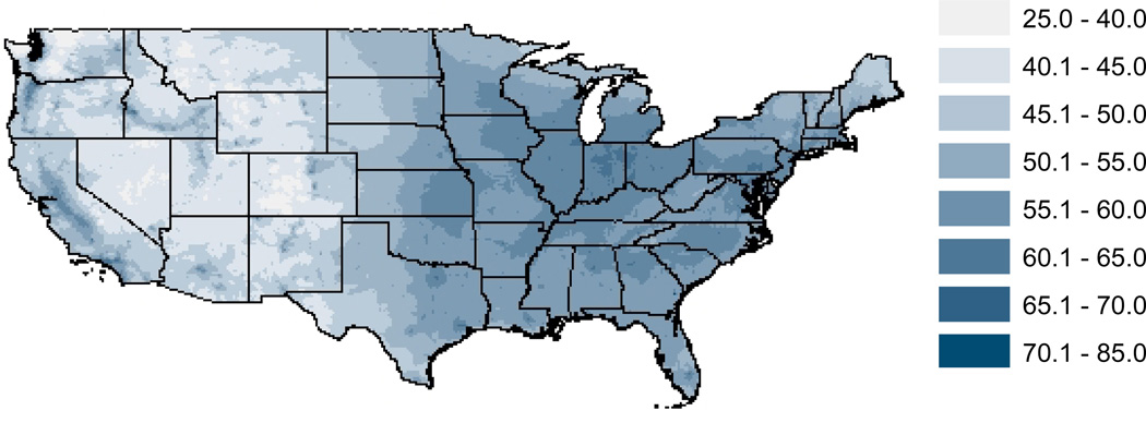
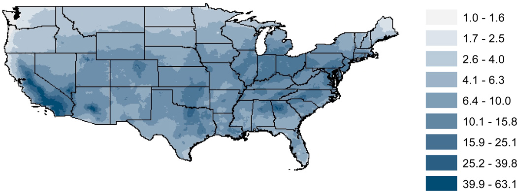
Figures 1 and 2 show the geographic distribution of 6-month mean daily one hour maximum ozone and annual average PM2.5 for the continental US at a 12 km resolution using the CMAQ output. In general, the highest PM2.5 values occur in the eastern United States. Ozone concentration is more geographically uniform, but peak values occur in southern California. Table 1 shows statistics for O3 and PM2.5 concentrations in the continental US at various grid cell resolutions. Maximum concentrations and the standard deviations decrease when going to coarser resolutions. For PM2.5, the maximum concentration decreases 71% from the 12 km resolution to the coarsest resolution of 408 km. The maximum O3 concentration at 408 km is 24% lower than the concentration at the 12 km resolution. Population-weighted mean concentrations, which are closely related to national health impacts, are 27% lower for PM2.5 and 2% lower for O3, at 408 km resolution compared with 12 km. Ozone, with its longer atmospheric lifetime, varies less spatially and is less affected by increasing cell size.
Figure 1.
Six month average from April to September of 1-hour daily maximum ozone concentrations (ppb) derived from 12 km CMAQ output.
Figure 2.
Annual average PM2.5 concentration (µg/m3) derived from 12 km CMAQ output.
Table 1.
Mean, maximum, and standard deviations of concentrations of annual average PM2.5 and the 6-month average of 1-hr. daily maximum O3, and population-weighted averages, at various resolutions over the continental US. Cells were selected for this averaging to match the original 12 km domain as closely as possible, and for coarse resolutions obtained by simple averaging, differences in mean concentrations indicate small differences in the area of the entire domain.
| Resolution (km) |
O3 (ppb) | PM2.5 (µg/m3) | ||||||
|---|---|---|---|---|---|---|---|---|
| Mean | Max | St. Dev | P-W mean |
Mean | Max | St. Dev | P-W mean |
|
| 12 | 52.43 | 82.92 | 6.93 | 58.46 | 5.13 | 49.35 | 3.48 | 10.55 |
| CMAQ 36 km |
53.93 | 81.96 | 7.41 | 61.51 | 5.56 | 36.31 | 3.78 | 11.14 |
| 96 | 52.32 | 74.55 | 6.84 | 58.67 | 5.10 | 16.22 | 3.37 | 9.43 |
| 144 | 52.16 | 71.41 | 6.84 | 58.77 | 5.07 | 15.94 | 3.28 | 9.03 |
| 300 | 52.05 | 65.52 | 6.64 | 57.49 | 5.04 | 14.61 | 3.12 | 8.15 |
| 408 | 52.44 | 63.35 | 5.93 | 57.17 | 5.02 | 14.16 | 3.06 | 7.67 |
3.2 Premature mortality due to ozone
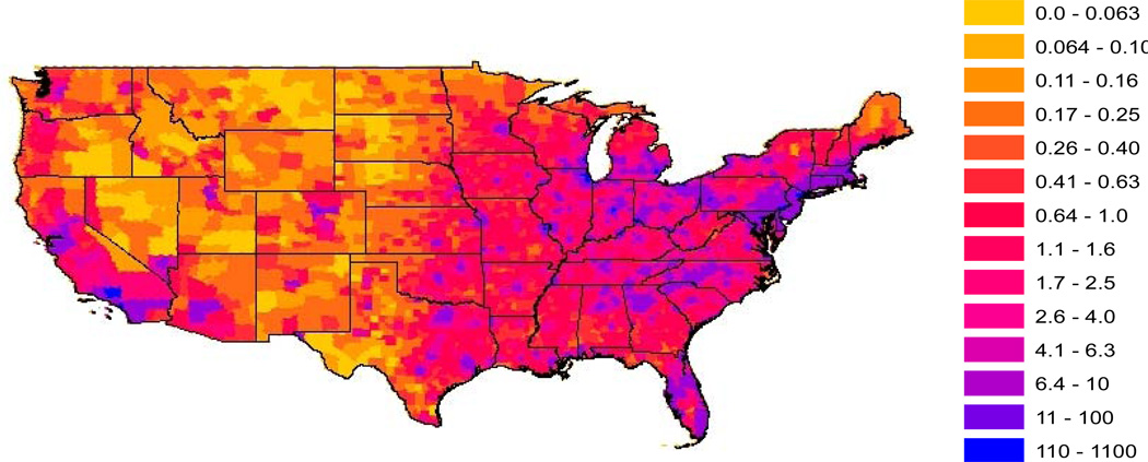
Using the finest resolution, we estimate 21,400 (95% CI, 5,600 – 34,200) annual respiratory deaths from simulated 2005 O3 concentrations (Figure 3). In this study, the 95% confidence intervals represent only the uncertainty in the concentration-response function. These results are comparable with those from other studies, in which the same concentration-response functions are used.Fann et al. (2012) estimate that 19,000 (95% CI, 7,600 –29,000) respiratory deaths occur each year in the US due to 2005 simulated maximum 8-hour ozone concentrations above modeled natural background levels. The highest density of deaths from ozone concentrations ofFann et al. (2012) also occur in southern California and in the eastern US.Anenberg et al. (2010) estimate 25,000 (1 SD, 10,000 – 40,000) deaths in North America due to present day (2000) ozone concentrations above preindustrial levels with low-concentration thresholds applied. Results fromAnenberg et al. (2010) are higher than our estimates due to a larger population size and different present day concentrations simulated using different atmospheric models.
Figure 3.
Annual respiratory mortality attributable to ozone in 2005 at 12 km resolution (deaths yr−1).
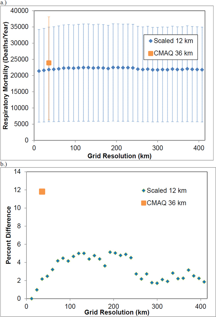
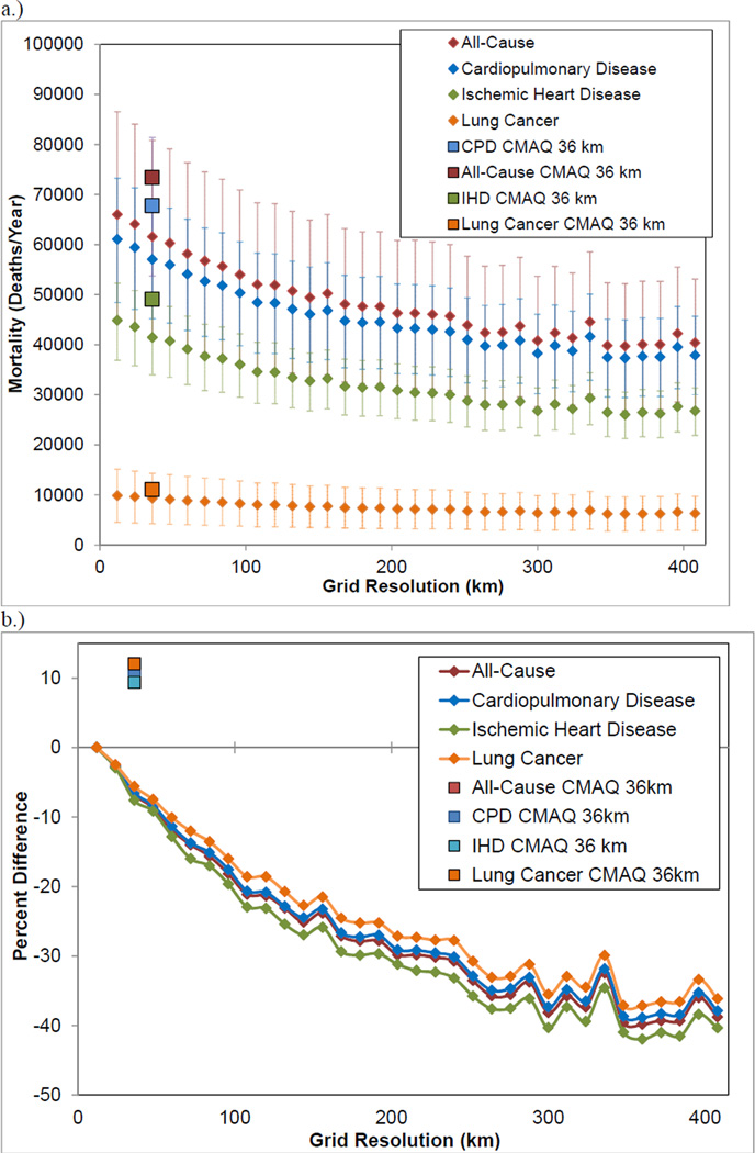
Using the 36 km output from CMAQ produces an estimate of mortality that is 12% higher than the 12 km estimate (Figure 4). Estimates at resolutions larger than approximately 96 km also show a small positive bias, not more than 6% different from the estimate at 12 km resolution. This small bias reflects the fact that ozone concentrations are rather uniform spatially. Small fluctuations in the estimates between similar grid resolutions are an artifact of how grid cells line up with population and emissions.
Figure 4.
a.) Annual respiratory mortality, and 95% confidence limits, due to ozone exposure estimated at various resolutions, including the results from the CMAQ 36 km resolution. b.) Percent difference in ozone respiratory mortality between the coarse resolution and the best estimate at 12 km at various resolutions, calculated as (coarse results - 12km results) / (12km results).
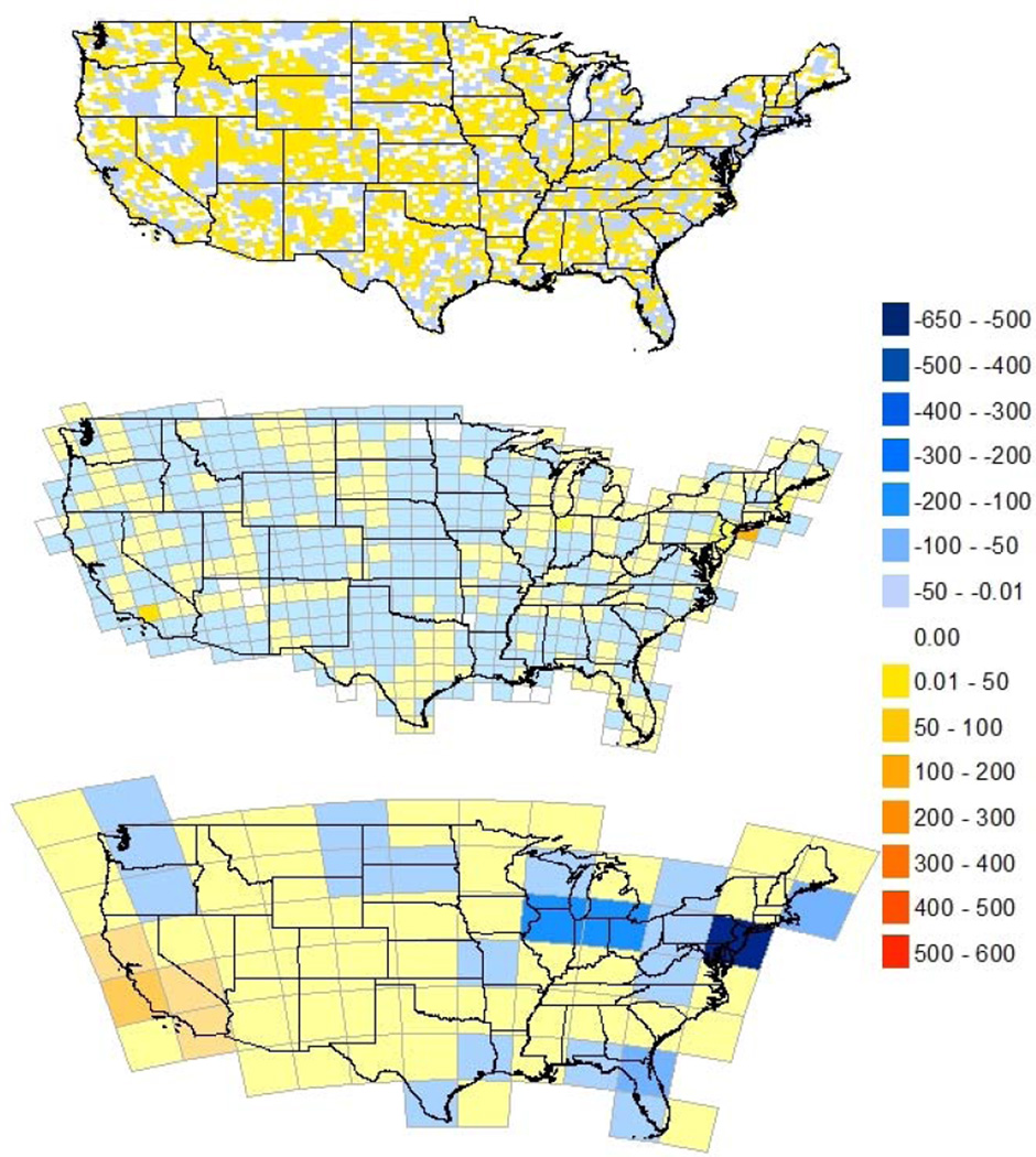
Figure 5 shows the differences in deaths estimated at a 12 km resolution and those at coarser resolutions, showing that the largest biases due to model resolution are near populated areas. At 36 km resolution, there is no noticeable pattern to the bias. At 144 km resolution, more cells overestimate mortality, especially in the Midwest and the largest differences occur near New York and Los Angeles. At 408 km resolution, there are small biases in most grid cells, with large differences in highly populated areas. When we normalize these biases by population, the bias does not show clear spatial patterns, and those patterns change at different coarse resolutions. For example, in Figure 5, the grid cell containing New York City is underestimated at 144 km, but overestimated at 408 km resolution. Consequently, we conclude that the large biases in urban areas are the result of large populations in these areas, and that biases in concentration due to coarse grid resolution are not necessarily larger than elsewhere, responding somewhat randomly to the orientation of grid cells.
Figure 5.
Difference in the number of annual ozone respiratory deaths, calculated as the 12 km estimate minus the 36 km, 144 km, and 408 km estimate, respectively.
3.3 Premature mortality due to total PM2.5
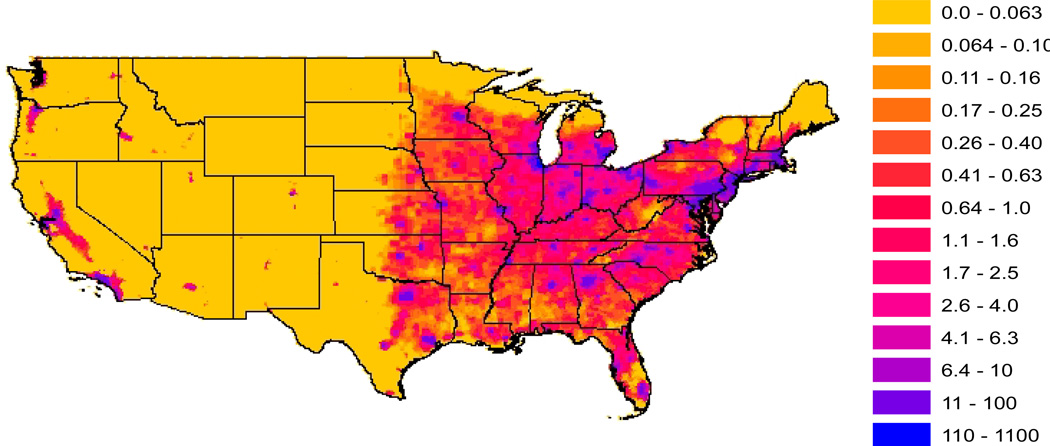
Using the finest resolution, we estimate that 66,000 (95% CI, 39,300 – 84,500) all-cause deaths occurred in 2005 due to exposure to PM2.5. We also estimate 61,000 (95% CI, 48,400 – 73,300) CPD deaths and 9,900 (95% CI, 4,500 – 15,100) lung cancer deaths. Cardiopulmonary mortality and lung cancer mortality can be summed to give an alternate estimate of the total burden that roughly agrees with the all-cause estimate. The greatest densities of deaths occur in highly populated areas (Figure 6), with few deaths outside of urban areas in the West, because these areas are often below the low-concentration threshold. Our estimates of PM2.5 mortality are similar to those ofAnenberg et al. (2010) for North America and the estimates of national mortality of the US EPA (2010b), but less than those ofFann et al. (2012).Anenberg et al. (2010) estimate 65,000 (1 SD, 35,000 – 95,000) cardiopulmonary deaths and 10,000 (1 SD, 5,000 – 15,000) lung cancer deaths each year due to 2000 annual average PM2.5 concentrations above a low concentration threshold of 5.8 µg/m3. The US EPA (2010b) estimates 63,000 (95% CI, 39,000 – 87,000) all-cause deaths occur each year in the US from 2005 PM2.5 concentrations above a 5.8 µg/m3 exposure threshold.Fann et al. (2012) estimate 130,000 (95% CI, 51,000 – 200,000) all-cause deaths in the US annually, relative to non-anthropogenic pollutant levels. Since we have selected results using the same concentration-response function (Krewski et al., 2009), differences between our results and the other national estimates are due in part to the endpoints analyzed, modeled present-day concentrations, and differences between low-concentration thresholds and preindustrial concentrations.
Figure 6.
Annual all-cause mortality due to total PM2.5 in 2005 at 12 km resolution (deaths yr−1).
The 36 km CMAQ model results produce an estimate of all-cause mortality that is 11% higher than the estimate at 12 km resolution (Figure 7), with very similar biases for all health endpoints. Increasing grid size by simple averaging to coarser resolutions decreases the estimated mortality. At resolutions <100 km, results driven with coarse total PM2.5 concentrations were <20% lower than the fine resolution estimate. Similarly, resolutions of 100–250 km produce mortality estimates that are 20–30% lower than the best estimate, and resolutions >250 km have estimates 30–40% lower. The decrease in the estimated mortality can be explained by the decrease in peak and population-weighted PM2.5 concentrations due to dilution into coarser grid cells, as these peaks typically occur in populated regions (Table 1, Figure 2). Consequently, coarse resolutions tend to underestimate the concentrations to which urban populations are exposed.
Figure 7.
a.) Estimated mortality due to total PM2.5 exposure calculated at various grid cell resolutions for all-cause, ischemic heart disease, lung cancer, and cardiopulmonary disease mortality, including the CMAQ 36 km results, with 95% confidence intervals. b.) Percent difference in PM2.5 mortality between the coarse resolution and the best estimate at 12 km at various resolutions, calculated as (coarse results - 12km results) / (12km results).
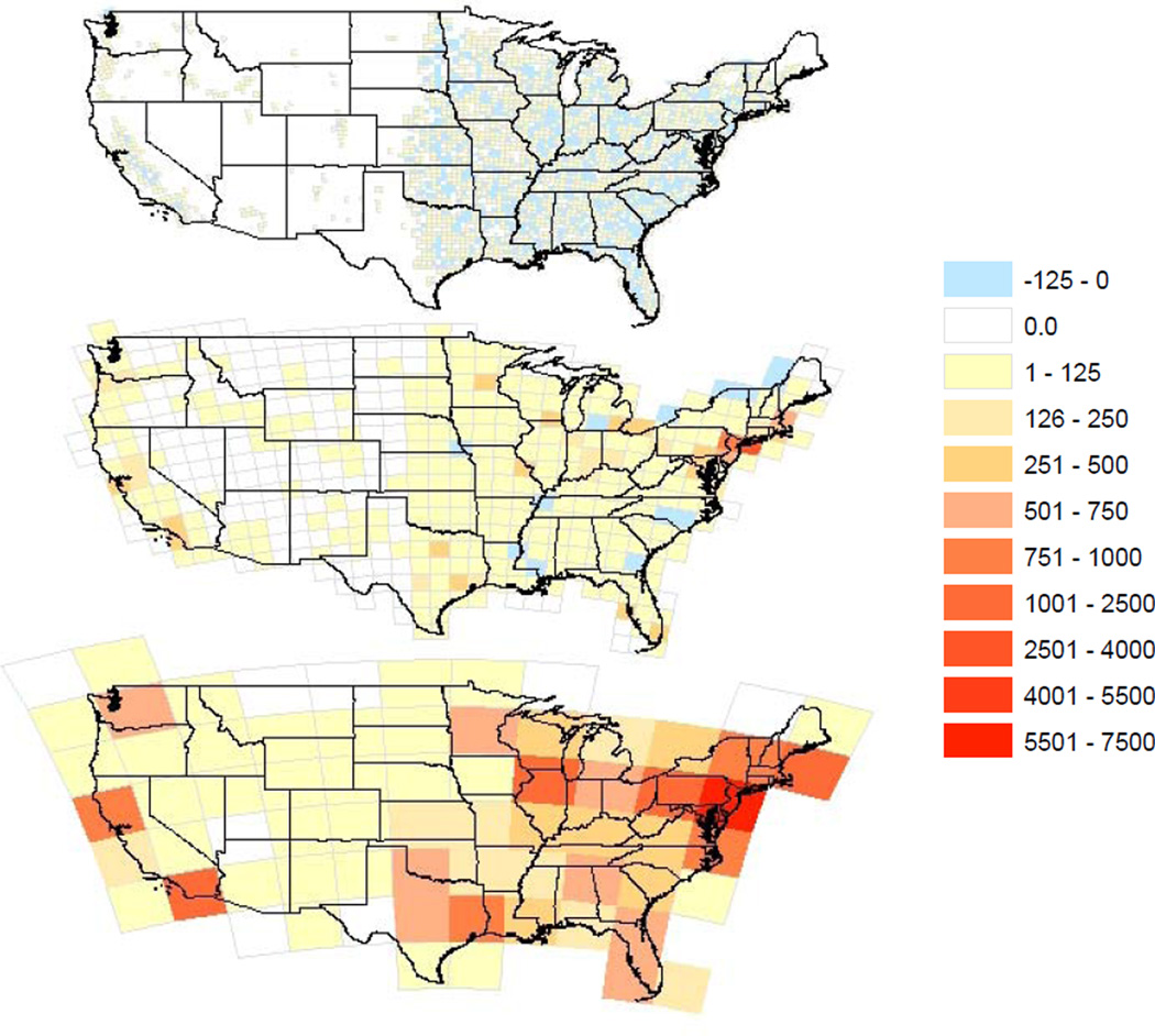
At 36 km resolution, the grid cells in the eastern US and on the west coast slightly overpredict or underpredict mortality (Figure 8); very few PM2.5 deaths are predicted elsewhere, such as the western mountainous regions where concentrations are frequently below the threshold (Figure 6). At 144 km resolution, mortality estimates are biased low in most grid cells, and errors are largest near cities. At 408 km resolution, there are underestimates in most grid cells, with the largest underestimates in highly populated regions. As for O3, the larger bias in populated regions essentially results from the larger population.
Figure 8.
Difference in estimated all-cause mortality attributable to PM2.5 in 2005 (deaths yr−1) caused by resolution, calculated as the 12 km estimate minus the 36 km, 144 km, and 408 km estimate, respectively.
3.4 Effect of grid resolution on primary and secondary species of PM2.5
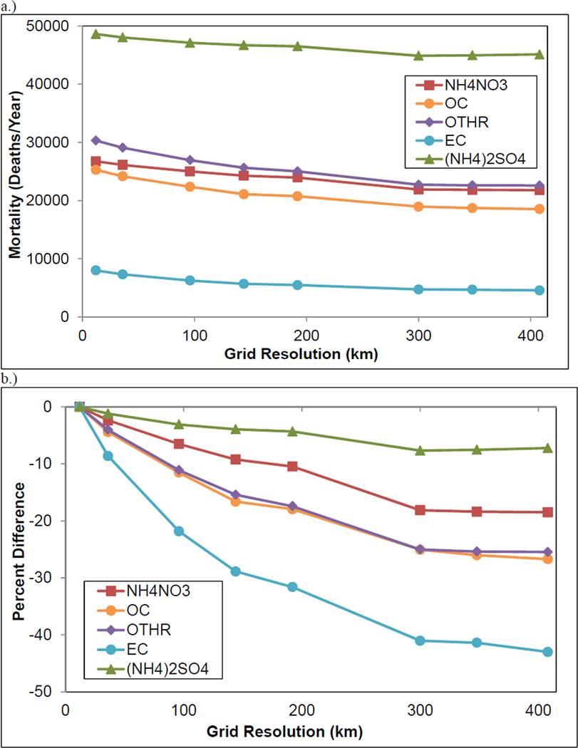
Deaths attributable to primary and secondary species of PM2.5 are also underpredicted at coarse grid cell resolution (Figure 9). Coarse resolution has the greatest percentage effect on estimates of mortality driven with primary species (EC and other; OC contains portions of primary and secondary) with estimates at 408 km resolution that are 25–43% less than the estimates at 12 km resolution. Primary species are directly emitted, have a short atmospheric lifetime, and are minimally influenced by chemical processes in the atmospheric model.
Figure 9.
a.) Annual all-cause mortality due to PM2.5 species in the US as a function of grid resolution, shown without a low concentration threshold. b.) Percent difference between all-cause mortality estimate at 12 km resolution and at coarser resolutions for PM2.5 species, without a low-concentration threshold.
Deaths attributable to secondary species, ammonium sulfate and ammonium nitrate, are less biased than PM2.5 total or primary species and, at 408 km resolution, are 7–18% different from the 12 km estimate. Ammonium sulfate has the highest concentration of the PM2.5 species and is the species least affected by grid cell size. The greater bias for primary species reflects the shorter atmospheric lifetimes and spatial ranges, compared to secondary species. Note that the deaths summed for individual species do not combine to give the deaths from PM2.5, mainly because we did not use low-concentration thresholds for evaluating individual species.
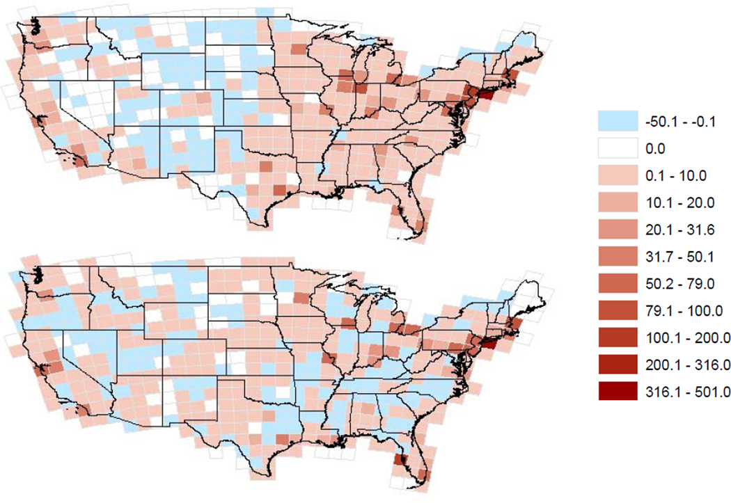
Figure 10 demonstrates that deaths for both EC and ammonium sulfate are underpredicted at 144 km resolution in most locations across the United States, with significant bias introduced near urban areas, due mainly to the larger population. Coarse resolution leads to less overall bias in mortality for ammonium sulfate than for elemental carbon. The poor ability of coarse resolutions to correctly capture the burden of mortality from total PM2.5 is therefore due mainly to the spatial heterogeneity of primary particulate species.
Figure 10.
Difference in the estimated all-cause deaths in 2005 due to resolution, for EC (top) and ammonium sulfate (bottom) without a low-concentration threshold, calculated as the 12 km estimate minus the 144 km estimate.
4. Summary and conclusions
We estimate that 66,000 (95% CI, 39,300 – 84,500) and 21,400 (95% CI, 5,600 – 34,200) deaths occur in the US annually due to PM2.5 and ozone, respectively, relative to low-concentration thresholds. Cardiopulmonary disease induced by PM2.5 contributes the majority of the national burden. Results at the finest resolutions show that the density of mortality is greatest around urban areas where population is the greatest, but mortality is also appreciable in rural areas. Because our calculation only includes the US population 30 years of age and older, although negative health impacts likely occur for all age groups, we likely underestimate the total mortality associated with ozone and PM2.5 in the US. In addition, we do not account for the known influences of ozone and PM2.5 on morbidity health outcomes. Other assumptions relevant for the total burden of mortality include applying the same concentration-mortality relationships to all populations, and assuming that all PM2.5 species have the same effects on mortality.
We evaluate the effect of increasing grid size on national estimates of mortality, relative to results obtained at 12 km resolution. Using air quality model results at 36 km resolution gives mortality burdens that are 11% higher for PM2.5 and 12% higher for O3, suggesting a modest positive bias. We extend this analysis to coarser resolutions, accounting for the effect of resolution on population exposure (the extent to which high population and high pollutant concentrations are coincident), but not the effect on model atmospheric processes. Increasing grid cell size, the estimate of total national respiratory mortality attributable to ozone is minimally affected, and no resolution increases results by more than 6% from the 12 km estimate. This small bias reflects the longer lifetime and more uniform concentration of ozone (and its precursors), with respect to PM2.5. This result indicates that the effect of resolution on atmospheric processes is likely to be the greatest source of error in mortality results driven with ozone concentrations. For ozone, coarse resolution has been shown cause either under- or overestimates of ozone concentrations at the resolutions of regional models, but an overestimate at the coarse resolution of global models (Wild and Prather, 2006).
Results driven with coarse total PM2.5 concentrations were <20% lower than the fine resolution estimate for resolutions <100 km, 20–30% lower at 100–250 km resolution, and 30–40% lower at resolutions >250 km. Overall, large grid cells perform poorly in capturing local variations in PM2.5 concentrations, with the largest differences between fine and coarse resolution estimates near highly populated urban regions. This larger bias compared to ozone results from the shorter lifetime of PM2.5 components. Biases at coarse resolution are greater for primary PM2.5 components and are much smaller for secondary components.
The biases identified here would suggest that estimates of PM2.5 mortality using model results at resolutions of <100 km should be increased by <33%, by 33–50% at 100–250 km resolution, and by 50–67% at resolutions >250 km. The estimates of global PM2.5 mortality ofAnenberg et al. (2010) could be increased by ~50%. However, we caution that because of the different spatial patterns of pollutant emissions and population elsewhere in the world, different correction factors may be appropriate on a global scale. These uncertainties may be amplified or diminished when accounting for the effects of coarse resolution models on the atmospheric processes relevant for the secondary species of PM2.5. Modeled chemistry has only small influences on primary PM2.5, and our estimate of bias due to grid resolution should be accurate.
Because of the larger bias near highly populated urban areas, it is important to model these regions with fine resolution, either by using fine resolution for the whole modeling domain, or by nesting grids in urban areas. For example, the EPA recommends fine resolution (<12 km) to model PM2.5 concentrations and, in areas with large primary sources, the recommended model resolution is 4 km (U.S. EPA, 2007). But modeling at this resolution is computationally expensive and impractical for some applications. In applications where coarser models are necessary, uncertainties due to grid resolution and a likely low bias for PM2.5 health effects should be acknowledged. Future research should repeat this analysis using output from an air quality model at multiple coarse grid resolutions, rather than the simple averaging method used here to artificially create coarse resolutions. Doing so would fully account for the effects of coarse resolution on both model chemistry and population exposure. In addition, while we estimated the importance of resolution on the total burden of disease, analyses more commonly evaluate the health effects of changes in emissions. Changes in emissions may not cause the same spatial distributions of ozone and PM2.5 as the total pollutant concentrations analyzed here and may therefore not cause the same biases estimated here, especially considering the nonlinear relationships between ozone and its precursors, for example. Future analyses should evaluate the biases at coarse resolutions for changes in emissions of individual precursors.
Acknowledgements
This work was supported by a grant from the National Institute of Environmental Health Sciences (P30ES010126) and by the Environmental Protection Agency, Office of Air Quality Planning and Standards. We thank Neal Fann, Charles Fulcher, Pat Dolwick, Sarav Arunachalam, Meridith Fry, Matt Woody, Susan Anenberg, Marc Serre, and Will Vizuete for their assistance with this project.
References
- Abt Associates Incorporated. Environmental Benefits and Mapping Program (Version 4.0) Bethesda, MD: Prepared for US Environmental Protection Agency Office of Air Quality Planning and Standards; 2010. [Google Scholar]
- Anenberg SC, Horowitz LW, Tong DQ, West JJ. An estimate of the global burden of anthropogenic ozone and fine particulate matter on premature human mortality using atmospheric modeling. Environ Health Persp. 2010;118:1189–1195. doi: 10.1289/ehp.0901220. [DOI] [PMC free article] [PubMed] [Google Scholar]
- Arunachalam S, Holland A, Do B, Abraczinskas M. A quantitative assessment of the influence of grid resolution on predictions of future-year air quality in North Carolina, USA. Atmos Env. 2006;40:5010–5026. [Google Scholar]
- Bell ML, McDermott A, Zeger SL, Samet JM, Dominici F. Ozone and short-term mortality in 95 US urban communities, 1987–2000. JAMA. 2004;292:2372–2378. doi: 10.1001/jama.292.19.2372. [DOI] [PMC free article] [PubMed] [Google Scholar]
- Bell ML, Peng RD, Dominici F. The exposure-response curve for ozone and risk of mortality and the adequacy of current ozone regulations. Environ Health Persp. 114:532–536. doi: 10.1289/ehp.8816. [DOI] [PMC free article] [PubMed] [Google Scholar]
- Binkowski FS, Roselle SJ. Models-3 Community Multiscale Air Quality (CMAQ) model aerosol component 1. model description. J Geophys Res. 2003;108(D6):4183. [Google Scholar]
- Blanchard CL, Roth PM, Tanenbaum SJ, Ziman SD, Seinfeld JH. The use of ambient measurements to identify which precursor species limit aerosol nitrate formation. J Air Waste Manage Assoc. 2000;50:2073–2084. [PubMed] [Google Scholar]
- Broeckaert F, Arsalane K, Hermans C, Bergamaschi E, Brustolin A, Matti A, Bernard A. Lung epithelial damage at low concentrations of ambient ozone. Lancet. 1999;353:900–901. doi: 10.1016/S0140-6736(99)00540-1. [DOI] [PubMed] [Google Scholar]
- Centers for Disease Control and Prevention. CDC Wonder. Atlanta, GA: US Department of Health and Human Services; 2009. [Google Scholar]
- Cohen AJ, Anderson HR, Ostro B, Pandey KD, Krzyzanowski M, Kunzli N, Gutschmidt K, Pope CA, III, Romieu I, Samet JM, Smith KR. Urban air pollution. In: Ezzati M, Lopez AD, Rodgers A, Murray CJL, editors. Comparative quantification of health risks: global and regional burden of disease due to selected major risk factors. Geneva: World Health Organization; 2004. pp. 1353–1434. [Google Scholar]
- Corbett JJ, Winebrake JJ, Green EH, Kasibhatla P, Eyring V, Lauer A. Mortality from ship emissions: a global assessment. Environ Sci Technol. 2007;41:8512–8518. doi: 10.1021/es071686z. [DOI] [PubMed] [Google Scholar]
- Fann N, Lamson AD, Anenberg SC, Wesson K, Risley D, Hubbell BJ. Estimating the national public health burden associated with exposure to ambient PM2.5 and ozone. Risk Analysis. 2012;32(1):81–95. doi: 10.1111/j.1539-6924.2011.01630.x. [DOI] [PubMed] [Google Scholar]
- Fann N, Roman HA, Fulcher CM, Gentile MA, Hubbell BJ, Wesson K, Levy JI. Maximizing health benefits and minimizing inequality: incorporating local-scale data in the design and evaluation of air quality policies. Risk Analysis. 2011;31:908–922. doi: 10.1111/j.1539-6924.2011.01629.x. [DOI] [PubMed] [Google Scholar]
- Greco SL, Wilson AM, Spengler JD, Levy JI. Spatial patterns of mobile source particulate matter emissions-to-exposure relationships across the United States. Atmos Environ. 2007;41:1011–1025. doi: 10.1021/es062213f. [DOI] [PubMed] [Google Scholar]
- Hubbell BJ, Fann N, Levy JI. Methodological considerations in developing local-scale health impact assessments: balancing national, regional, and local data. Air Qual Atmos Health. 2009;2:99–110. [Google Scholar]
- Hubbell BJ, Hallberg A, McCubbin DR, Post E. Health-related benefits of attaining the 8-hr ozone standard. Environ. Health Persp. 2005;113:73–82. doi: 10.1289/ehp.7186. [DOI] [PMC free article] [PubMed] [Google Scholar]
- Ito K, De Leon SF, Lippmann M. Associations between ozone and daily mortality: analysis and meta-analysis. Epidemiology. 2005;16:446–457. doi: 10.1097/01.ede.0000165821.90114.7f. [DOI] [PubMed] [Google Scholar]
- Jang JC, Jeffries H, Byun D, Pleim JE. Sensitivity of ozone to model grid resolution – 1 Application of high-resolution regional acid deposition model. Atmos Environ. 1995;29(21):2085–3100. [Google Scholar]
- Jerrett M, Burnett RT, Ma RJ, Pope CA, Krewski D, Newbold KB, Thurston G, Shi YL, Finkelstein N, Calle EE, Thun MJ. Spatial analysis of air pollution and mortality in Los Angeles. Epidemiology. 2005;16:727–736. doi: 10.1097/01.ede.0000181630.15826.7d. [DOI] [PubMed] [Google Scholar]
- Jerrett M, Burnett RT, Pope CA, III, Ito K, Thurston G, Krewski D, Shi Y, Calle E, Thun M. Long-term ozone exposure and mortality. New Engl J Med. 2009;360:1085–1095. doi: 10.1056/NEJMoa0803894. [DOI] [PMC free article] [PubMed] [Google Scholar]
- Krewski D, Jerrett M, Burnett RT, Ma R, Hughes E, Shi Y, Turner MC, Pope CA, III, Thurston G, Calle EE, Thun MJ. Health Effects Institute Research Report 140. Boston: 2009. Extended follow-up and spatial analysis of the American Cancer Society study linking particulate air pollution and mortality. [PubMed] [Google Scholar]
- Laden F, Schwartz J, Speizer FE, Dockery DW. Reduction in fine particulate air pollution and mortality. Am J Respir Crit Care Med. 2006;173:667–672. doi: 10.1164/rccm.200503-443OC. [DOI] [PMC free article] [PubMed] [Google Scholar]
- Liang J, Jacobson M. Effects of subgrid segregation on ozone production efficiency in a chemical model. Atmos Environ. 2000;34:2975–2982. [Google Scholar]
- Ostro B, Feng WY, Broadwin R, Green S, Lipsett M. The effects of components of fine particulate air pollution on mortality in California: results from CALFINE. Environ Health Persp. 2007;115:13–19. doi: 10.1289/ehp.9281. [DOI] [PMC free article] [PubMed] [Google Scholar]
- Ostro B. WHO Environmental Burden of Disease Series, No. 5. Geneva: World Health Organization; 2004. Outdoor air Pollution: Assessing the Environmental Burden of Disease at National and Local Levels. [Google Scholar]
- Pope CA, III, Burnett RT, Thun MJ, Calle EE, Krewski D, Ito K, Thurston GD. Lung cancer, cardiopulmonary mortality, and long-term exposure to fine particle air pollution. JAMA. 2002;287:1132–1141. doi: 10.1001/jama.287.9.1132. [DOI] [PMC free article] [PubMed] [Google Scholar]
- Seinfeld JH, Pandis SN. 2nd edn. Hoboken, NJ: Wiley; 2006. Atmospheric chemistry and physics: from air pollution to climate change. [Google Scholar]
- Tang Y. A case study of nesting simulation for the Southern Oxidants Study 1999 at Nashville. Atmos Env. 2002;36:1691–1705. [Google Scholar]
- Thompson TM, Selin NE. Influence of air quality model resolution on uncertainty associated with health impacts. Atmos Chem Phys. 2012;12:9753–9762. [Google Scholar]
- US Environmental Protection Agency. EPA-454/B-07-002. Research Triangle Park, NC: 2007. Guidance on the use of models and other analyses for demonstrating attainment of air quality goals for ozone, PM2.5, and regional haze. [Google Scholar]
- US Environmental Protection Agency. EPA-454/R-10-00. Research Triangle Park, NC: 2010a. Air quality modeling technical support document: light-duty vehicle greenhouse gas emission standards final rule. [Google Scholar]
- US Environmental Protection Agency. EPA-452/R-10-005. Research Triangle Park, NC: 2010b. Quantitative health risk assessment for particulate matter. [Google Scholar]
- West JJ, Fiore AM, Horowitz LW, Mauzerall DL. Global health benefits of mitigating ozone pollution with methane emission controls. Proceed Natl Acad Sci. 2006;103:3988–3993. doi: 10.1073/pnas.0600201103. [DOI] [PMC free article] [PubMed] [Google Scholar]
- Wild O, Prather MJ. Global tropospheric ozone modeling: Quantifying errors due to grid resolution. J Geophys Res. 2006;111:D11305. [Google Scholar]
- Woods and Poole Economics Inc. Population by Single Year of Age CD. Washington, DC: 2001. [Google Scholar]


