

Abstract
Recently, there has been great interest among vision researchers in developing computational models that predict the distribution of saccadic endpoints in naturalistic scenes. In many of these studies, subjects are instructed to view scenes without any particular task in mind so that stimulus-driven (bottom-up) processes guide visual attention. However, whenever there is a search task, goal-driven (top-down) processes tend to dominate guidance, as indicated by attention being systematically biased toward image features that resemble those of the search target. In the present study, we devise a top-down model of visual attention during search in complex scenes based on similarity between the target and regions of the search scene. Similarity is defined for several feature dimensions such as orientation or spatial frequency using a histogram-matching technique. The amount of attentional guidance across visual feature dimensions is predicted by a previously introduced informativeness measure. We use eye-movement data gathered from participants’ search of a set of naturalistic scenes to evaluate the model. The model is found to predict the distribution of saccadic endpoints in search displays nearly as accurately as do other observers’ eye-movement data in the same displays.
Keywords: visual search, visual attention, top-down attentional control, real-world scenes, informativeness, eye tracking, eye movements, saccadic selectivity, scene perception
Introduction
Visual search plays a key role in such everyday activities as finding a friend in a crowd or a favorite shirt in a cluttered closet. Due to the complexity of Sreal-world scenes and the limited processing resources in our visual system, it is crucial for efficient search that it selectively processes the most relevant information for the given task. This selection is achieved by shifting our attention through the search space in a pattern that is closely followed by saccadic eye movements (Findlay, 2004; Motter & Holsapple, 2007).
One of the most influential theories explaining how observers perform visual search tasks efficiently is Guided Search (Wolfe, 1994). According to this theory, we create, during pre-attentive scene processing, an “activation map” indicating likely target locations. During the subsequent search process, this map determines which regions of the scene will capture most attention. Both bottom-up (stimulus-driven) and top-down (goal-driven) factors may contribute to the topography of this activation or salience map.
Bottom-up activation is a target-independent effect, determined solely by local visual properties of the search scene. For example, a single red blossom in a green field may draw more attention and gaze fixations than its surroundings, regardless of the search target. Top-down activation, in contrast, depends upon the relationship between the target and search scene locations.
Although the Guided Search theory was first proposed to explain search for discrete objects among fields of distracter objects, the idea of generating a salience map to guide the subsequent allocation of overt visual attention (i.e., eye movements) has more recently been adapted to the study of search in complex and continuous natural scenes.
Mechanisms of bottom-up activation have been well-researched in psychophysical experiments in which subjects viewed natural scenes without being assigned any search task (e.g., Bruce & Tsotsos, 2006; Itti & Koch, 2000; Parkhurst, Law, & Niebur, 2002; for a review see Henderson, 2003). Moreover, neurobiological studies of bottom-up control of attention (e.g., Corbetta & Shulman, 2002; Palmer, 1999) have been conducted.
Recent results, however, suggest that, during visual search tasks, in which subjects are asked to find a particular target in a display, top-down processes play a dominant role in the guidance of eye-movements (e.g., Henderson, Brockmole, Castelhano, & Mack, 2007; Peters & Itti, 2007; Pomplun, 2006; Zelinsky, Zhang, Yu, Chen, & Samaras, 2006). Furthermore, fMRI studies have provided neurophysiological evidence for the existence of top-down activation maps in the visual system (e.g., Egner et al., 2008; Corbetta & Shulman, 2002; Weidner, Pollmann, Muller, & von Cramon, 2002), further motivating an in-depth study of top-down factors guiding search.
One type of top-down guidance is exerted by high-level, semantic or contextual information (Neider & Zenlinsky, 2006; Oliva, Wolfe, & Arsenio, 2004). Here, our expectations about where objects belong in our environment guide our eye-movements as we search a scene for a known object. When searching a room for an electric outlet, for example, we are more likely to look along the lower regions of the walls than toward the ceiling. Torralba and colleagues developed a model which seeks to quantify such high-level contextual effects on search (Torralba, Oliva, Castelhano, & Henderson, 2006).
In addition to these high-level factors, lower-level visual features in real-world scenes such as intensity and hue of the target systematically bias eye fixations during search toward scene regions that resemble target features (Hwang, Higgins, & Pomplun, 2007; Pomplun, 2006). Intuitively, this seems to be a simple, straightforward mechanism: For instance, when searching for a red apple, our eye movements will be drawn preferentially to red elements in the scene. The problem becomes complex when we consider that the target object is defined by multiple features along several dimensions, each of which may be shared by different elements of the search space. This creates a competition among feature dimensions, and for maximal search efficiency, the optimal weighting of dimensions in guiding search needs to be chosen.
Recently, several models of eye movements during search in real-world images have been proposed (Frintrop, Backer, & Rome, 2005, Navalpakkam & Itti, 2006; Zelinsky, 2008). The most comprehensive model to date is the Target Acquisition Model (TAM) by Zelinsky (2008). It simulates an observer’s retinal distribution of photo receptors to predict complete visual scan paths and the moment of target detection. Several measures indicate good correspondence in behavior between the model and actual human subjects, which is remarkable for a model making such detailed predictions. However, TAM does not address the abovementioned problem of weighting feature dimensions in the guidance of search.
Other researchers did attempt to model aspects of low-level, top-down contributions to real-world visual search based on the idea that top-down control works by weighting the feature-wise bottom-up saliency maps proposed by Itti and Koch (2000). In the model of Navalpakkam and Itti (2006), signal-to-noise ratios (SNRs) are assigned to features and feature dimensions for a given search scene based upon the distribution of low-level features in the target and the scene. These SNRs are then used to weight the contribution of features and dimensions during the integration of previously-created, bottom-up feature saliency maps (i.e., maps which show bottom-up activation in a scene for an individual feature dimension). The approach taken in Frintrop et al. (2005), which models the well-known “pop-out” effect that occurs in human search when a target is uniquely defined by a single feature within a scene, uses a normalization technique during feature map integration to heighten the guidance of dimensions along which the target is most distinctive.
Although these studies implementing top-down weighting of features by modulating bottom-up activation have made important contributions to the field, several issues must be addressed if we are to develop plausible models of human visual search. First, top-down factors are treated as merely tuning more fundamental, bottom-up effects. Given that top-down factors have been shown to be crucial in everyday search, we suggest that these factors ought to figure more prominently in computational models of visual search. This view is supported by recent studies showing that the influence of bottom-up factors on eye movements during search in static scenes is negligible (Henderson et al., 2007; Zelinsky et al., 2006).
Second, we maintain that these models make certain unrealistic assumptions about search. The model by Navalpakkam and Itti assumes that, prior to inspection of the search image, the distribution of visual features in the search scene has to be learned by the search agent to compute the amount of noise or distracters in the scene. However, a complex learning process is unlikely to occur in the visual system before every search, as it would severely reduce search efficiency. It is more plausible that a fast, coarse mechanism using heuristics is responsible for biasing attention toward the most informative feature dimensions. For Frintrop’s model, the target location has to be known by the search agent—an unlikely scenario in the context of most everyday searches.
Third, in these models, a composite saliency map for a given search image is computed by integrating feature saliency maps in a disjunctive (i.e., additive) manner. As will be further discussed below, however, a conjunctive (i.e., multiplicative) approach to feature saliency integration best captures guidance of search by human observers.
Finally, in neither study is the accuracy of these proposed models in predicting human search behavior quantitatively measured against empirical eye-movement data in real-world scenes. This lack of quantitative evaluation makes it impossible to objectively assess and compare the performance of different models.
In this study, we extend previous work to propose and quantitatively evaluate a new model of top-down, low-level feature guidance during search, which attempts to address these concerns. The model employs top-down saliency maps (“similarity landscapes”) for individual feature dimensions and estimates the informativeness of the those maps based on a previously introduced, computationally inexpensive measure (Hwang, Higgins, & Pomplun, under review). This measure is then used to weight the contribution of each feature’s similarity landscape during integration and formation of the final salience map. Since the computation of informativeness in a given feature dimension depends entirely on the shape of its top-down saliency map, the model does not require any training or prior knowledge of the search space. We first analyze human eye-movement data gathered during search in natural scenes and demonstrate the relevance of the informativeness measure for predicting guidance patterns. Subsequently, we motivate our modeling approach and evaluate the model’s predictive power against the empirical eye-movement data.
Method
Participants
Thirty participants, 4 females and 26 males, completed this experiment. All were students or faculty members at the University of Massachusetts Boston, aged between 19 to 40 years old. Each participant was entitled to a $10 honorarium.
Apparatus
Eye movements were tracked and recorded using an SR research EyeLink II system. After calibration, the average error of visual angle in this system is 0.5°. Its sampling frequency is 500 Hz. Stimuli were presented on a 19-inch Dell P992 monitor. Its refresh rate was set to 85 Hz and its resolution was set to 1280 × 1024 pixels. Participant responses were entered using a handset or game-pad.
Materials
A total of 160 photographs (800 × 800 pixels) of real-world scenes, including landscapes, home interiors, and city scenes were selected as stimuli (see Figure 1). When displayed on the screen, each stimulus covered 20° × 20° of visual angle.
Figure 1.
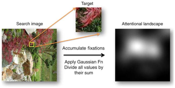
Computation process for attentional landscapes. After accumulating fixations from all subjects, we apply a 2D Gaussian function. The attentional landscape is normalized as probability density function.
Although semantic factors are known to play an important role in guidance during search, such effects lie beyond the scope of the present research. Thus, in order to minimize the possibly overriding influence of semantic guidance, stimuli were randomly rotated by 0°, 90°, 180° or 270°. The distribution of these rotations was approximately even (0°: 40 images, 90°: 40 images, 180°: 43 images, and 270°: 37 images), and the orientation of each image was held constant for all subjects.
For each scene, a potential search target location of 64 × 64 pixels (1.5° × 1.5° visual angle) was randomly chosen from the stimulus, excluding a center region of 192 × 192 pixels. Potential targets were then inspected and those deemed uninformative (e.g., completely black or white) or semantically rich (e.g., containing identifiable objects) were rejected and assigned a new random position. Target locations were approximately evenly distributed over the search area except for the excluded central area.
Procedure
Participants viewed 4 blocks of 40 stimuli. For each trial, the search target was displayed at the center of the screen on a black background for two seconds to allow subjects to memorize the target. After this preview, the whole search display was shown and participants were asked to locate the target. If participants believed that they found the target location, they pressed a button on the game-pad while fixating on the location. If they were unable to locate the target in 7 seconds, the trial would time-out and the next trial would begin.
Data analysis
Measures of subjects’ performance
Individual subjects’ performance can be measured by two variables: answer correctness and target cover time. The average answer correctness is the proportion of correct manual responses across all displays. Although subjects were asked to press the button while fixating on the target location once they determined it, they often pressed the button shortly before or after their fixation on that location. Therefore, a correct answer is defined as the subject pressing the button while fixating within 2° of visual angle from the center of the target. Due to the difficulty of the current search task, subjects pressed the button in only 85.5% of the trials, and their average answer correctness was 44.5 ± 15% (in the present work, ‘±’ always indicates a mean value and its standard deviation). All experimental trials, regardless of their answer correctness, were included in the data analysis.
The average cover time is the time from the onset of the search display until the subject fixates on the target area for the first time. Again, hitting the target area is defined as making eye fixation within 2° of visual angle from the center of the target location. If a subject never makes a fixation on the target location during search, cover time for that trial is operationally defined to be the maximum 7 seconds for which the display was visible. In a previous study (Hwang et al., 2007), this measure was found to be more insightful than response time, because many search images contain multiple locations that are similar to target. Therefore, it often happens that subjects check the target location but cannot make a decision in time or make an incorrect decision. The average cover time for all subjects was 4.17 ± 1.34 s.
For each trial, an average of 16.6 ± 7.26 fixations was made, whose mean duration was 253 ± 146 ms. The average saccade length was 3.62 ± 3.19°. For those trials in which subjects gave a correct answer in time, the average number of fixations, fixation duration, and saccade length were 10.57 ± 4.90, 235 ± 126 ms, and 4.21 ± 3.73°, respectively.
Attentional landscapes
It has been shown that eye movements and visual attention are closely linked during visual search (Findlay, 2004; Motter & Holsapple, 2007). Furthermore, low-level visual features are known to significantly guide eye movements during search in real-world scenes (Pomplun, 2006). Therefore, it seems justified to use fixation distributions gathered from visual search tasks to study how natural low-level visual features guide our visual attention during search tasks.
Using the eye-movement data recorded during the visual search experiment, we constructed attentional landscapes. Assuming that attention is most likely guided by target features during search, an attentional landscape is a result of integrated feature guidance, with peaks indicating regions that garner most attention. Since fixation duration is believed to depend on local information complexity rather than attentional guidance (Hooge & Erkelens, 1999; Williams & Reingold, 2001), only the local density of fixations, regardless of their durations, determines the elevation of the attentional landscape.
Based on these assumptions, all subjects’ fixation positions for each search display were collapsed. Subsequently, in order to account for the hypothesized size of the visual span, a 2D Gaussian function with standard deviation of 64 pixels, representing about one degree of visual angle, was applied to the fixation distribution to obtain a fixation density map or attentional landscape (see Figure 1). Since in the present study all targets were of a particular, identical size, we assumed that the observers’ “attentional focus” operated at the corresponding resolution.
In constructing our attentional landscapes, we controlled for two factors that may bias the fixation distribution. One of these arises from experimental design and the other is due to the natural search behavior of participants. First, since the experimental task was designed so that the subjects’ gaze always starts at the center of the search image and—in successful search—ends at the target location, fixation densities near the center of the image and the target location are inflated. In order to reduce this bias, the first three fixations and final three fixations were excluded from the analysis.
Second, during search tasks under laboratory conditions, our eye fixations are not only guided by the low-level display features but are also biased toward the center of a presented image (Tatler, 2007). In this study, we computed the average fixation distribution across all subjects and all search displays. In order to prevent a disproportionate influence of fixation-intensive trials, we normalized the distributions across individual subjects and images. As expected, the resulting average distribution showed elevated fixation density near the center of the image. We controlled for this central bias by dividing each display’s unique attentional landscape by this average fixation distribution (see Figure 2). Since we used a large number of randomly chosen, everyday scenes with evenly distributed target locations, the results of this operation only minimally depended on our particular choice of stimuli.
Figure 2.
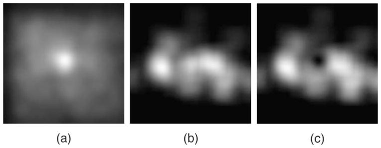
Controlling for the natural search bias. Brighter areas indicate greater fixation density. (a) Combined fixation distribution across the 160 search trials. (b) Fixation distribution in trial #26. (c) Final attentional landscape for trial #26 after controlling for the bias.
Finally, fixation density maps were normalized so that the sum of elevation across the display was one. The resulting smooth landscapes approximate the 2D probability density function of human eye fixations falling onto specific locations in the displays during the search task.
Similarity landscapes for feature dimensions
Similarity landscapes are defined as distributions of target-display similarity across the search space in terms of each visual feature dimension, peaking where the image most closely resembles the target. For example, if the spatial frequencies of the target and a given location are very similar, this location will represent a peak in the spatial frequency similarity map for this image.
In our analysis we considered a total of eight low-level visual features (see below). Their similarity maps were generated by moving a target-sized window (64 × 64 pixels) over evenly distributed locations of each search image. For each step, the window moved by 32 pixels so that it overlapped with one half of the previous location. Consequently, there were 23 × 23 locations for each search image (a total of 529 positions). As discussed above, we assumed that the constant target size in our study induced a corresponding visual span or “attentional focus” size. Consequently, our model operates exclusively at the target-size resolution, unlike other models that include multiple scales (e.g., Itti and Koch, 2000).
During this windowing process, each location’s similarity to the target was independently computed for each of the eight selected dimensions. From the many different methods to compute similarity we chose a simple, robust histogram matching method called “Histogram Intersection Similarity Method (HISM)” (Swain & Ballard, 1991), which has been successfully used, for example, in image-retrieval systems. With this method, similarity between target and local area was defined by an intersection of two histograms after both histograms were normalized so that their values ranged from zero to one (see Figure 3).
Figure 3.
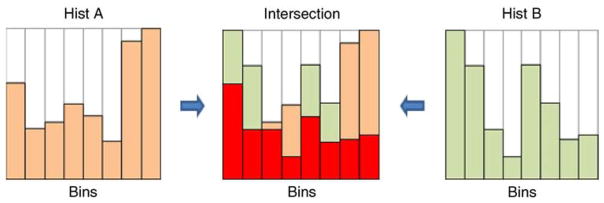
Histogram Intersection Similarity Method (HISM). Histograms have eight bins and are normalized so that their minimum value is 0 and their maximum value is 1. Histograms A (left) and B (right) are examples of target and local feature histograms, respectively. Their intersection (center) consists of the smaller of the two values in corresponding bins. The size of the red area is our measure of similarity between target and local histograms.
Similarity maps for each dimension were then created by assigning target-similarity values along the selected dimension to all locations. A 2D Gaussian function with a standard deviation of 1.5° was applied to the resulting maps, producing smooth distributions. Finally, the maps were normalized so that the sum of all similarity values over each map was one. For each image, we thus generated eight feature-similarity landscapes representing probability density functions for the given visual feature dimensions across the search image. The entire process is illustrated in Figure 4.
Figure 4.
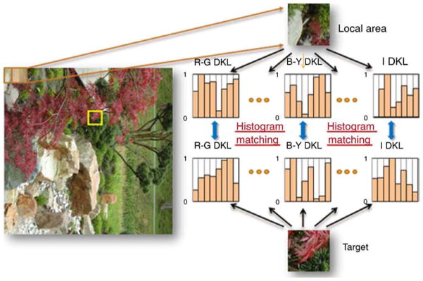
Computing similarity landscapes for individual feature dimensions. After computing the local similarity values, we applied a 2D Gaussian function and normalized the sum of similarity vales for each map to one.
The set of the eight feature dimensions used in this study was not optimized for model performance. Most likely, more comprehensive and less redundant sets of feature dimensions could be defined. The current eight dimensions were chosen simply based on their importance for the discrimination of color, direction, and complexity. Four dimensions were selected for color—red-green activation (R-G), blue-yellow activation (B-Y), and luminance (L), based on the Derrington-Krauskopf-Lennie (DKL) color model (Derrington, Krauskopf, & Lennie, 1984), and intensity, computed as the average of the three color components in the RGB space. Two dimensions for direction, orientation and luminance gradient, were also studied. We finally selected two dimensions for complexity, namely spatial frequency and intensity contrast.
The DKL color model is thought to be perceptually plausible as it simulates the eye’s cone receptor sensitivity on three wave lengths (short, medium and long) and models the responses by its main double opponent cells, a red-green type and a blue-yellow type, plus a luminance response (Conway, 2001). Details of the color-space conversion process from the RGB color space to the DKL color model are explained in Appendix A. For color features, all pixels in the given patch (target or local area) were converted to the DKL color space and their values were accumulated in an 8-bin histogram for HISM computation.
Orientation and frequency features were computed in the frequency domain. After a given patch was converted to the frequency domain using Fast Fourier Transform (FFT), its power spectrum was generated (see Figure 5a). However, there are two factors that need to be corrected before any histogram computation. The first factor is due to the nature of the FFT computation. Since FFT assumes that the image is infinitely repeated, the power spectrum shows more power on the horizontal and vertical angles due to the square edge of the local patches (Gonzalez & Woods, 2002). To reduce this effect, the power spectra were pre-processed using the Blackman function. The second factor results from the general power distribution in real-world images, in which low-frequency bands typically have much greater power than high-frequency bands. To eliminate this imbalance, we normalized the power spectra by dividing them by the average power spectrum for the whole image set.
Figure 5.
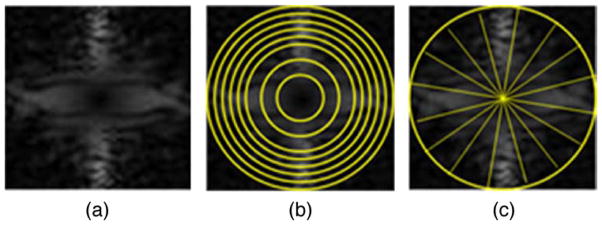
Histogram bin values for frequency and orientation were defined as the sum of power in one of eight equal-sized slices. (a) Power spectrum of target #26. (b) Example of the donut-shape slicing method for computing frequency histograms. (c) Example of the pie-shape slicing method for computing orientation histograms. Due to the symmetry of the power spectra, the 16 orientation slices resulted in only eight bin values.
The frequency histograms were computed in such a way that each bin contained the sum of power from one of eight equal-sized “donut” shapes. Therefore, each bin in the frequency histogram represents the normalized sum of power for a given frequency band (see Figure 5b). The orientation histograms were computed in a way similar to that of the frequency histograms, but power spectra were divided into 16 equal-sized “pie slices” and the power in each opposite-slice pair was summed to obtain a value for each bin in the orientation histogram (see Figure 5c).
Intensity gradient is a surface orientation measure that is defined by the average intensity difference along eight directions. Each bin represents the strength of the intensity gradient in a given direction. For every location in the given clip, the differences in brightness between a center pixel and its eight neighboring pixels were accumulated in the corresponding bin. If the difference between the center pixel and a neighboring pixel was negative, the absolute difference value was summed in the bin that represented the opposite direction. Unlike the orientation variable, which is based on power spectra and is more strongly affected by line orientations, this variable measures the overall intensity gradient of the clip.
The final dimension, intensity contrast, was processed via scalar values instead of histograms. Intensity contrast was computed as the standard deviation of intensity across the 64 × 64 pixels in a given patch. Similarity in this dimension was computed as the negative absolute difference between the values for the target and the local patch. The resulting similarity maps were normalized in the same way as the maps for the histogram-based dimensions.
Feature-dimension guidance
Feature-dimension guidance is a quantitative measure of the extent to which the visual features in a given dimension guide a subject’s attention during the course of the search task. If a target-similarity landscape generated for a given dimension—e.g. luminance—is highly predictive of the distribution of human eye movements during visual search, we can say that this dimension shows strong guidance (Hwang et al., 2007; Pomplun, 2006).
In previous studies, guidance in real-world images has been measured by several computational methods such as the average elevation of fixation density on target features (Pomplun, 2006), Pearson correlation between attentional landscape and target-similarity landscape (Hwang et al., 2007), and Receiver Operating Characteristic (ROC—e.g., Tatler, Baddeley, & Gilchrist, 2005). While yielding intuitively interpretable results, the elevation method is not an ideal standard for guidance analysis as its results strongly vary with the assumed number of features per dimension. Since both the Pearson and ROC methods do not require this assumption and provide useful and somewhat complementary measures, in the following we will use both of them for assessing guidance. The Pearson method reveals the degree to which the shape of a similarity landscape matches the shape of an attentional landscape across the display. It is important to notice, however, that attentional landscapes can be ill-defined in areas of extremely low fixation density. This potential source of noise does not affect the ROC technique, which emphasizes the correct prediction of attention peaks by the similarity landscapes and largely disregards the attention valleys.
The Pearson measure is simply computed as the correlation between the elevation of the attentional landscape and the target-similarity landscape for a given dimension at all 529 measurement locations per display. Perfect guidance by that dimension would be indicated by a value of one, whereas the absence of guidance would result in a value of zero. The ROC measure is perhaps best understood by analogy: Consider a three-dimensional landscape, such as a target-similarity landscape, being ‘flooded’ with water. An ROC value for a given feature dimension is then computed as follows: First, we flood its similarity landscape until it is completely submerged (i.e., from above, 0% of its area is visible). The landscape is then continuously drained so that 1%, 2%, …, 100% of the landscape emerges from the water. For each water level, a subject’s eye fixations for the same image are projected onto the landscape and the proportion of the fixations visible—being located above the water level—is computed. After the computation of the visibility rate, we plot it as a function of the water level as shown in Figure 6. The resulting ROC value is the area under this function.
Figure 6.
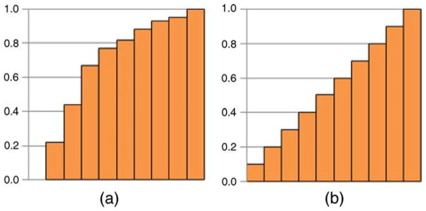
Illustration of the ROC measure. The horizontal axis represents the proportion of visible (above-threshold) area at each threshold value. The vertical axis represents the proportion of fixations hitting the visible area. (a) Example of positive predictor. (b) Example of chance-level predictor.
For a chance-level predictor (no guidance), the ROC value is 0.5 and for the perfect predictor, the ROC value is one. However, in the present context, the theoretical upper limit of one is virtually impossible to reach because landscapes are smoothed by a Gaussian function. In order to find the practical upper limit of the ROC measure, we computed the ROC value of the attentional landscapes for all images as predictors of all subjects’ fixations. While this value is one without the Gaussian function, the actual result is 0.837 ± 0.050.
In order to ensure that that theoretical baseline values for both the Pearson (0.0) and ROC measures (0.5) represent true chance-level prediction of empirical eye-movement data in this study, we generated a set of random fixations for each display such that the number of fixations was equal to that in empirical eye-movement data. We found that the prediction of empirical eye movements by these random fixation distributions in terms of both the Pearson (0.007 ± 0.144) and ROC measures (0.501 ± 0.074) did not differ significantly from the theoretical chance levels, both ts(159) < 0.4, ps > 0.5.
Using the Pearson and ROC measures, Figure 7 illustrates how well the target-similarity landscapes for the eight chosen dimensions predict the distribution of attention, that is, how strongly those dimensions guide search. Four guidance tiers are visible, which are (in descending order of guidance, with their Pearson and ROC values in parentheses): (1) Intensity (0.37, 0.66); (2) DKL R-G (0.33, 0.64), DKL B-Y (0.34, 0.64), and DKL L (0.31, 0.63); (3) contrast (0.26, 0.61) and gradient (0.29, 0.62); (4) frequency (0.20, 0.58) and orientation (0.20, 0.58). All differences in guidance between the tiers are significant for both the Pearson measure, all ts(159) > 2.51, ps < 0.05, and the ROC measure, all ts(159) > 2.88, ps < 0.05.
Figure 7.

Results of visual feature guidance using both Pearson correlation and ROC methods. Error bars indicate standard error of the mean. Dashed lines represent upper and lower bounds of possible ROC values in this analysis.
Notice that, following Pomplun (2006), all subjects’ data were combined for a useful computation of attentional landscapes. Consequently, statistical tests were computed across the 160 displays instead of the 30 subjects. In the following, unless otherwise stated, all reported statistical tests and variables such as standard deviation and standard error were calculated across displays.
Informativeness of feature dimensions
In artificial search displays showing discrete search items with a small set of visual features, a phenomenon known as the distracter-ratio effect has been shown to bias eye-movement patterns (Shen, Reingold, & Pomplun, 2000). It has been shown that visual attention is preferentially guided by those features of the target that are most distinctive, i.e., that are shared by the fewest distracter items. For example, consider a search condition in which the target is a red horizontal bar and distracters may be either red vertical bars or blue horizontal bars. As the proportion of red distracters increases, guidance along the other dimension—orientation—rises. Therefore, the distracter-ratio effect reflects an optimization mechanism for guiding search that favors more informative stimulus dimensions.
In the present study, we refined and extended the concept of the distracter-ratio effect so that it can accommodate the target-distracter similarity in real-world search displays. Following our earlier study (Hwang et al., under review), we mathematically defined the informativeness of a feature dimension as the proportion of a similarity landscape for which similarity-to-target is at most 50% of its maximum for a given display (see Figure 8).
Figure 8.

Example of informativeness computation. (a), (c) Feature dimension similarity landscapes for the DKL R-G channel and frequency, respectively. (b), (d) Result of threshold operation at 50% maximum height of each landscape. The proportion of black area over the whole image area is taken as the informativeness of that feature dimension. In this example, informativeness is 0.348 for the DKL R-G feature dimension and 0.222 for the frequency dimension. In these examples, the DKL R-G dimension is more informative for search than is the frequency dimension and thus may receive greater weight in guiding visual attention.
Why use a 50% threshold? In our previous study, this value was chosen because intuitively it should be most sensitive to differences in informativeness. The resulting measure was shown to be a useful predictor of guidance across dimensions in a given display, and an excellent predictor for the average guidance by a given dimension across displays. For the present study, we therefore decided to use the same threshold. In addition, we used the current eye-movement data to analyze the dependence of these findings on the choice of similarity threshold. As Figure 9 illustrates, the average informativeness-guidance correlation per dimension is maximized at threshold values around 40% to 50% for both the Pearson and ROC guidance measures.
Figure 9.

Average correlation between informativeness and guidance for the eight feature dimensions across the 160 search trials as a function of the similarity threshold. Both guidance measures (Pearson and ROC) reveal maximum correlation in the threshold range of approximately 40% to 50%. Curves indicate quadratic function fits, and error bars indicate standard error of the mean across dimensions.
Another important aspect of informativeness with similarity threshold of 50% is that there exists a strong positive correlation between average informativeness and average guidance across dimensions. An analysis of the present data shows only slight variation in this correlation for similarity thresholds between 10% and 60% (see Figure 10). Above this threshold range, correlation is rapidly broken. Confirming the results obtained in Hwang et al. (under review), the correlation coefficient between average informativeness and average guidance across the eight dimensions for a 50% threshold is very high for both the Pearson method (r = 0.98, p < 0.0001) and the ROC method (r = 0.96, p < 0.0005).
Figure 10.

Correlation coefficient between average informativeness and average guidance across the eight dimensions, shown as a function of the similarity threshold. For threshold up to 70%, there exists a strong positive correlation (r > 0.95).
The present data support the intuitively proposed 50% threshold as a good choice for measuring informativeness when modeling top-down guidance of attention. As shown in Figure 11, at this threshold, there exist positive informativeness-guidance correlations (for both Pearson and ROC) for all feature dimensions, all ps < 0.005: intensity (0.32, 0.29), contrast (0.33, 0.23), gradient (0.58, 0.60), frequency (0.34, 0.36), orientation (0.32, 0.34), DKL R-G (0.43, 0.35), DKL B-Y (0.36, 0.43), and DKL L (0.51, 0.51). These results indicate adaptation of guidance to informativeness in individual trials.
Figure 11.

Correlation coefficient between informativeness and guidance for individual feature dimensions.
The model
Integrating the similarity landscapes
Our proposed model relies upon the correlation between informativeness and guidance across feature dimensions. Since informativeness can be computed based on display and target information alone, this correlation enables us to—at least roughly—predict feature guidance across dimensions without requiring knowledge of human fixation data. These guidance values, in turn, tell us the contribution of a given similarity map to guiding search and can thus be used as weighting factors for the similarity maps’ integration into a top-down saliency map.
Furthermore, if we assume that there are limited processing resources available during real-time information integration (e.g., Duncan & Humphreys, 1989), weighting values should be normalized using the following Equation 1 so that the sum of weightings—i.e., processing resources—among all feature dimensions becomes one:
| (1) |
Where Wd is the final weight for feature dimension d and Id is the informativeness of feature dimension d for the current search task.
The next question we need to ask is how this weighting should be applied for the integration of similarity landscapes. The currently most popular method for computing saliency maps is the weighted sum method (Frintrop et al., 2005; Itti & Koch, 2000; Navalpakkam & Itti, 2006). It treats each feature dimension’s saliency contribution as independent signal propagation. Accordingly, the total sum of saliency strength is accumulated as if bottom-up saliency effects propagate separately along the visual pathway. Each saliency map is disjunctively summed while the given feature dimension’s weighting is applied:
| (2) |
where Ex,y is the final saliency elevation at location (x, y) in search space and Sd,x,y is the similarity value at location (x, y) in the similarity landscape for feature dimension d.
However, for modeling search behavior, which is strongly determined by top-down guidance (Henderson et al., 2007; Zelinsky et al., 2006), we argue that the weighted sum method is not the most adequate way of integrating saliency across feature dimensions. This view is based on the observation made in a previous study (Pomplun, 2006) that attentional landscapes typically contain only few peaks, while their elevation is near zero for most of the display area (see also Figures 1 and 2c). However, for individual dimensions, the distribution of saliency—i.e., target-similarity—is usually less focused and differs among the dimensions (see Figure 11). Therefore, if attention were actually guided by the sum of top-down saliency across dimensions, we would expect to see less pronounced peaks and significant elevation throughout the display. As a more appropriate approach to solving the integration problem, we propose the weighted product method:
| (3) |
This method considers features as an integrated set of characteristics that defines the target. In order to implement weighting of individual similarity maps, the weights in Equation 3 have to take the form of an exponent for the similarity value for each feature dimension. This exponential weighting results in the nice property that if a feature dimension is entirely uninformative, it will turn the similarity value of the whole similarity map for that dimension into one. Therefore, that dimension will not contribute to guiding search.
At first glance, Equation 3 seems inadequate because it implies that at locations with zero similarity to the target in one or more of the dimensions, the overall elevation will be zero as well. Consequently, in a standard conjunction search task (e.g., Wolfe, 1994), Equation 3 seems to predict that only the target object is salient and should be detected immediately, which contradicts empirical findings. However, it is important to notice that due to factors such as noise in perception and memorization as well as the complexity of search images, target-similarity never drops to zero.
The product method assumes the search task to depend on feature matching in terms of a conjunctive operation among the feature dimensions. Since similarity maps and human fixation distribution maps are correlated, each similarity map approximates the probability of eye fixations on a given location guided by that feature. Since our similarity maps are also normalized as probability mass functions, integrating similarity maps using the AND operation approximates the probability distribution of eye fixations across the search image.
Although the weighted product method is substantially more complex than the weighted sum method due to its non-linearity, our hypothesis is that the product method is a more adequate approach than the “standard” sum method at predicting the overall shape of empirical attentional landscapes in modeling top-down effects during visual search tasks. Unlike the sum method, the product method does not require any post-processing steps in order to generate plausible predictions of attentional landscapes. In the following section, the hypotheses underlying the concept of our proposed model (see Figure 12) are evaluated using the empirical eye-movement data.
Figure 12.
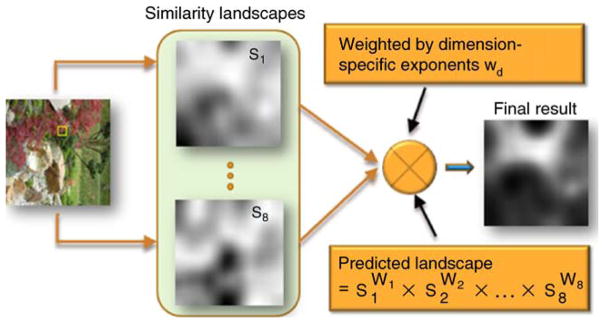
Schematic of model operation. From the similarity landscapes, weighting across dimensions is computed based on informativeness. Afterwards, similarity landscapes are integrated using the weighted product method.
Performance evaluation
Evaluation of weighting strategies
In order to quantify our model’s predictive performance, we applied the same methods that we used for computing overall feature guidance, namely the Pearson method and the ROC method. However, this time, instead of comparing the attentional landscapes and similarity landscapes, we compared the empirical attentional landscapes and the model-generated ones. To evaluate our proposed approach of computing the weighted product of the informativeness of feature dimensions in individual displays, it is compared against the weighted sum method and alternative weighting strategies. It is important to notice that for none of these algorithms, including our proposed model, were any parameters fitted to empirical performance or eye-movement data. Instead, their implementation was based on straightforward assumptions in order for our analysis to reveal qualitative differences between approaches rather than the extent to which they can be fitted to match actual subjects’ data.
Several strategies for choosing the weights across feature dimensions were tested. The Unit Weights (UW) case is a baseline strategy in which the similarity maps are integrated using unit weighting. In other words, the contributions of all feature dimensions to the guidance of search are assumed to be equal. Any strategies whose performance does not significantly exceed the UW results are thus not useful for modeling guidance.
The Average Pearson (AP), Average ROC (AR) and Average Informativeness (AI) cases utilize the dimension-wise average Pearson guidance, ROC guidance, and informativeness values, respectively, across all 160 displays as weights. These strategies assign the same pattern of weights regardless of the characteristics of the current search task. Clearly, the Pearson and ROC guidance values cannot be part of any complete modeling approach, because they require empirical eye-movement data for their computation. They are included in this comparison as reference models whose performance could be achieved if Pearson and ROC values could be exactly predicted from display and target data alone.
Finally, in the Individual Pearson (IP), Individual ROC (IR) and Individual Informativeness (II) cases, the weights are adjusted for every individual display-target pair, representing adaptive, dimension-wise weighting for each display-target pair. For the current display-target pair, its average Pearson (IP) or ROC (IR) guidance value across subjects, or its informativeness (II) for each dimension is simply taken as the weight for that dimension in predicting the distribution of attention in the current display. Again, the IP and IR cases just serve as reference models, while the II case represents our proposed modeling approach. All performance data are computed using two different integration methods, the weighted sum and the weighted product, as discussed above.
Even without looking at individual data points, the results in Figure 13a show us that guidance for integrated feature dimensions is clearly higher than previously computed dimension-wise guidance values (see Figure 7). Disregarding the uninformed UW case, for integrated dimensions, predictive performance is in the 0.40~0.48 range using the Pearson method and in the 0.67~0.70 range for the ROC method. In comparison, guidance by individual dimensions is in the 0.20~0.37 range for the Pearson method and in the 0.58~0.65 range using the ROC method. This performance boost is due to feature integration, supporting the view that the human visual system uses cross-dimensional information integration for search (Quinlan, 2003).
Figure 13.

Performance of different weighting strategies measured by Pearson method (a) and ROC method (b). Weighting strategies: Unit Weights (UW), Average Pearson (AP), Average ROC (AR), Average Informativeness (AI), Individual Pearson (IP), Individual ROC (IR) and Individual Informativeness (II). In each case, performance is measured for both the weighted product approach and the weighted sum approach. Error bars indicate standard error.
Moreover, the data indicate that the weighted product method performs significantly better than the weighted sum method when performance is measured using the Pearson method. The average difference across weighting strategies is 0.019 ± 0.007, and all of the individual differences are significant, all ts(159) > 8.36, ps < 0.001. Moreover, visual inspection of the final activation maps reveals that the weighted product method leads to “cleaner” maps in which the peaks are more condensed. This effect seems to be due to the fact that multiplication of similarity effectively removes the noise peaks. However, as shown in Figure 13b, this difference between the two weighting methods does not translate into a performance difference when performance is measured using the ROC method, all ts(159) < 1.70, ps > 0.09. As discussed above, ROC values depend more strongly on the location of the tallest peaks than on the overall distribution of fixations. The current data therefore suggest that while the product method and the sum method predict fixation peaks equally well, the product method is superior at predicting the overall distribution of fixations. We will thus limit the following analysis of the weighting strategies to the product method.
When comparing the different weighting strategies, we find that, for the Pearson measure, the average-based strategies, AP (0.40), AR (0.41) and AI (0.40) outperform the UW strategy (0.38), all ts(159) > 3.30, ps < 0.005. This difference indicates that in natural search scenes, some feature dimensions are generally more informative than others, and incorporating this knowledge into the model leads to better prediction of search behavior. For example, intensity and color dimensions exert stronger guidance than other dimensions (see Figure 7). This bias in human observers can be either a result of long-term learning of informativeness of feature dimensions in natural scenes, or an evolutionary specialization of the visual system for processing these dimensions.
It must be noted, however, that for the ROC measure only the difference between UW (0.66) and AR (0.67) reaches significance, t(159) = 4.28, p < 0.001, while there are only tendencies for such differences between UW and AP (0.67), t(159) = 1.45, p = 0.15, and between UW and AI (0.67), t(159) = 1.32, p = 0.19. This finding, once again, can be attributed to the greater sensitivity of the Pearson measure to similarity in fixation density across the display.
If we compare the average-based weighting cases (UW, AP, AR and AI) with the individual (display by display) weighting cases, we find increased performance by the latter group for both measures: IP (Pearson: 0.48; ROC: 0.69), IR (0.47, 0.70) and II (0.43, 0.68), all ts(159) > 2.90, ps < 0.05. Therefore, it seems that in human observers feature-dimension weighting is to a large extent dynamically assigned based on the current display-target pair to maximize search performance.
Again, it is important to notice that our proposed model is represented by the II strategy, whereas the IP and IR cases are based on empirical eye-movement data and are included for providing reference data only. Both the IP and the IR cases outperform the II strategy, both ts(159) > 6.77, ps < 0.001, indicating that a better prediction of guidance across dimensions could significantly improve the model. On the other hand, the II strategy performed better than any of the strategies that do not adapt their weights to individual display-target pairs (UW, AP, AR, and AI), all ts(159) > 4.10, ps < 0.001) on both Pearson and ROC measures. This result signifies that in our proposed model, the weighting of dimensions for individual displays based on our informativeness measure makes a significant contribution to the prediction of attentional guidance.
Figure 14 shows examples of empirical fixation data on top of fixation probability distributions generated by various methods. Note that the yellow dots in all four panels indicate the cumulated fixations of all subjects for a given search image and thus are always identical. What differs across panels is the underlying landscape that reflects different data generation methods. Figures 14a and 14b show the upper and lower bound performance, respectively, as discussed above. The performance of our proposed weighting strategy, individual informativeness (II), is shown for two different feature integration methods, weighted sum method (Figure 14c) and weighted product method (Figure 14d). As it can be seen, the lower peaks in the weighted-sum landscape are effectively eliminated in the weighted-product landscape, making it a stronger predictor of fixation distribution as measured by the Pearson method.
Figure 14.

Examples of fixation probability distributions (grayscale landscapes) and empirical fixation data (yellow dot fields). (a) Optimal prediction: distribution landscape generated directly from eye-movement data. (Pearson: 1.000, ROC: 0.813). (b) Chance-level prediction: distribution based on random fixation generation (Pearson: 0.010, ROC: 0.523). (c) Distribution produced by our model (“individual informativeness,” II) using the weighted sum method (Pearson: 0.505, ROC: 0.690). (d) Distribution derived from our model using the weighted product method (Pearson: 0.551, ROC: 0.670).
The model’s predictive power
The previous analyses have shown that the model meets its minimum requirement, that is, it predicts human performance above chance level. A more important question, however, is: How close is the model to the optimal performance that any model could achieve? Since there is variance in behavior between individual observers, it is impossible for any model to predict every individual observer’s behavior perfectly. For the following analysis, we used arguably the best predictor of subjects’ eye movements: other subjects’ eye movements in the same display-target pairs.
To evaluate how well the model predicts individual subjects’ eye movements, we let the model predict an attentional landscape for each of the 160 display-target pairs and compute the average ROC value for each individual subject’s fixations across these landscapes. For comparison, we repeated this procedure, but this time the landscapes were the actual attentional landscapes based on the other 29 subjects’ collective data (all subjects except the one whose data are being predicted). These ROC data represent the approximate maximal performance any model can reach.
As an additional measure for group predictions, the model was also compared to a group-to-group prediction in which the 30 subjects were randomly divided into two groups of 15 subjects each. The attentional landscapes based on the first group’s collective fixations served as the predictor of the second group’s fixations. For comparison, the model also predicted the second group’s fixations.
Figure 15 shows the predictive power of the subject population and our model for individual and group data. It demonstrates that our model’s predictive power for individual subjects (0.67) is slightly lower, t(159) = 8.18, p < 0.001, than the predictive power of the subject population (0.72). When we consider the group-wise prediction, the population’s predictive power (0.70) is slightly lower than for the individual data, t(159) = 6.36, p < 0.001, conceivably because the number of data points used to estimate the population is decreased in group-wise prediction. Conversely, the model’s prediction power increases on group prediction (0.68) compared to individual prediction, t(159) = 4.51, p < 0.001.
Figure 15.

Comparison of predictive power (ROC method) between our model and the subject population for individual and group data. (a) Prediction of individual data: Population is estimated by the other subjects’ eye fixation data except the one that is predicted. (b) Prediction of group data: Population is estimated by the other half of subject group’s fixation data. Error bars indicate standard error of the mean, and dotted lines indicate the chance level (0.5).
These data suggest that, particularly for group prediction, the current model is quite close to the maximal performance that any model could reach. Given that our model only incorporates top-down control of attention and none of its parameters were fitted to any empirical performance or eye-movement data in order to optimize its output, this result supports the plausibility of our modeling approach.
Conclusions
Unlike other search models that focus on modeling an observer’s sequence of fixations (e.g., Najemnik & Geisler, 2005; Zelinsky, 2008), the aim of this present modeling study was to predict, for a given target and real-world search display, the statistical distribution of fixations. An adequate model predicting such distribution could provide important insight into the attentional mechanisms underlying search behavior. For this purpose, no parameters of the model were fitted to empirical performance or eye-movement data. All mechanisms, both the ones proposed for the model and alternative ones used for reference and comparison, were implemented in the most straightforward and naïve manner. This research strategy most likely failed to determine the maximal predictive performance that the model could have reached if its parameters had been optimally tuned using empirical data. More importantly, however, this strategy allowed us to compare the key contributions of different mechanisms instead of their malleability toward producing specific, desired data.
Despite the omission of data fitting, the model we have presented here is able to predict the statistical distribution of human eye fixations during search in real-world images quite well. In particular, the accuracy of its prediction of combined data from multiple subjects was shown to be only slightly below the optimum that any model could achieve. This result was accomplished with relatively simple and straightforward means. First, a histogram matching technique was used to define the similarity between the target and the local display content along eight low-level stimulus dimensions. This similarity was assumed the main factor underlying the guidance of visual attention and eye movements. Second, this guidance was thought to be biased toward the most informative dimensions, as determined by a previously introduced informativeness measure (Hwang et al., under review). Third, the model’s predicted distribution of fixations was computed as the informativeness-weighted product of the target-similarity maps for individual stimulus dimensions.
The evaluation of the model and its components has brought about some noteworthy findings. Regarding the informativeness measure, we demonstrated its robustness for a range of similarity thresholds and justified the earlier choice of a 50% threshold. Furthermore, our results suggest that the weighted product method for integrating the target-similarity maps may be more appropriate than the sum method used in previous studies (e.g., Frintrop et al., 2005; Navalpakkam & Itti, 2006). While both methods predict the highest fixation peaks well, the current data seem to indicate that the product method approximates the empirical fixation density distribution more closely. Weighting the contribution of individual feature dimensions by their informativeness leads to a better prediction of subjects’ gaze behavior. Recomputing this weighting for the informativeness in every individual search display, as done in the proposed model, leads to an even greater improvement than using static weights based on the average informativeness of dimensions across displays. These results suggest that weighting of feature dimensions is an integral mechanism for attentional control, and models without such mechanism such as TAM (Zelinsky, 2008) could be further improved by adding it. The evaluation also showed that if the guidance by individual dimensions could be predicted more reliably, a significantly better prediction of fixation distribution could be achieved.
The current informativeness measure used for weighting the contribution of different stimulus dimensions is simpler than other approaches, most notably the model of attentional tuning of visual features developed by Navalpakkam and Itti (2007). However, the performance of our informativeness measure in the current model suggests that it may reflect a mechanism similar to the actual neural functions tuning cross-dimensional attention. It is reasonable to assume that the biological mechanisms have evolved to be simple and efficiently computable by a highly parallel neural network. Our informativeness measure meets these criteria. It does not require any training for specific search tasks or any prior knowledge about the target location. Once we are able to quantitatively compare different approaches on complex images, the nature of the underlying neural circuitry will become more amenable to analysis.
As a first step toward comparability of visual search models, the evaluation of the current model was performed using two common quantitative measures: Pearson correlation and ROC. Consequently, the present study yielded a wealth of quantitative performance data whose counterparts could easily be computed for other existing or future models of guidance during search. This opportunity could lead to the first useful, quantitative comparisons of visual search models, whose unattainability so far has most likely impeded the progress in this field of research.
Although our model does not include bottom-up mechanisms of attentional guidance, it nonetheless yields close predictions of empirical eye-movement data. This finding may support previous results suggesting that, at least in static scenes, purely stimulus-driven effects upon attentional guidance are minimal (Henderson et al., 2007; Zelinsky et al., 2006). In the light of the current data, the conceptualization of top-down attentional control as a modulator of bottom-up control as in the models by Frintrop et al. (2005) and Navalpakkam and Itti (2006) seems even harder to justify.
One of the significant shortcomings of the current model is its assumption of a constant distribution of visual processing resources around fixation, simulated by a Gaussian function of constant width. However, previous research such as the Area Activation Model (AAM) by Pomplun, Shen, and Reingold (2003) suggested that this width is inversely correlated with the difficulty of the search task. Our future research will develop a predictor for task difficulty based on informativeness-related measures in order to estimate the distribution of processing resources for individual search tasks.
Another important limitation of the model in its present state is its restriction to search for exact visual patterns of one particular size. In everyday search, we are typically looking for objects and need to recognize them in different orientations, at various visual angles, and under any conditions of lighting and partial occlusion. Often, we do not even search for a particular object but for an instance of some object category. An adequate model of search for object or object categories, in turn, needs to incorporate semantic and contextual effects (Neider & Zelinsky, 2006; Oliva et al., 2004). The final goal for this line of research is to integrate the current approach with the AAM concept and address these higher-level influences to derive a “general-purpose” model of attentional control during visual search.
Acknowledgments
This research was supported by Grant Number R15EY017988 from the National Eye Institute to M.P.
Appendix A
RGB to DKL color conversion
Deriving a color space conversion from the RGB to the DKL model requires multiple steps because the DKL color model is based on the response curves for short, medium and long wavelength. First, the RGB color components are converted to the CIE XYZ color space using the following formula (Fairman, Brill, & Hermmendinger, 1997):
| (A1) |
Next, the CIE XYZ color space is converted to the LMS space using the chromatic adaptation matrix MCAT02 from the CIE CAM02 model (Fairchild, 2005):
| (A2) |
Finally, the LMS color space can be converted to the DKL color model using the following three equations (Lennie et al., 1990):
| (A3) |
| (A4) |
| (A5) |
where the R-G value models the red-green double opponent cells in the retina, B-Y models the blue-yellow double opponent cells, and L represents luminance. From Equations A3, A4, and A5, we can compute the LMS to DKL conversion matrix as follows:
| (A6) |
Since all three functions are linear, they can be expressed by multiplying the three matrices. The resulting matrix directly maps from RGB color space to DKL color space:
| (A7) |
Footnotes
Commercial relationships: none.
Contributor Information
Alex D. Hwang, Email: ahwang@cs.umb.edu, Department of Computer Science, University of Massachusetts, Boston, MA, USA, http://www.cs.umb.edu/~ahwang
Emily C. Higgins, Email: emilychiggins@gmail.com, Department of Computer Science, University of Massachusetts, Boston, MA, USA
Marc Pomplun, Email: marc@cs.umb.edu, Department of Computer Science, University of Massachusetts, Boston, MA, USA, http://www.cs.umb.edu/~marc.
References
- Bruce NDB, Tsotsos JK. Saliency based on information maximization. Advances in Neural Information Processing Systems. 2006;18:155–162. [Google Scholar]
- Conway BR. Spatial structure of cone inputs to color cells in alert Macaque primary visual cortex (V-1) Journal of Neuroscience. 2001;21:2768–2783. doi: 10.1523/JNEUROSCI.21-08-02768.2001. [DOI] [PMC free article] [PubMed] [Google Scholar]
- Corbetta M, Shulman GL. Control of goal-directed and stimulus-driven attention in the brain. Nature Reviews, Neuroscience. 2002;3:201–215. doi: 10.1038/nrn755. [DOI] [PubMed] [Google Scholar]
- Derrington AM, Krauskopf J, Lennie P. Chromatic mechanisms in lateral geniculate nucleus of macaque. The Journal of Physiology. 1984;357:241–265. doi: 10.1113/jphysiol.1984.sp015499. [DOI] [PMC free article] [PubMed] [Google Scholar]
- Duncan J, Humphreys GW. Visual search and stimulus similarity. Psychological Review. 1989;96:433–458. doi: 10.1037/0033-295x.96.3.433. [DOI] [PubMed] [Google Scholar]
- Egner T, Monti JM, Trittschuh EH, Wienecke CA, Hirsch J, Mesulam MM. Neural integration of top-down spatial and feature-based information in visual search. Journal of Neuroscience. 2008;28:6141–6151. doi: 10.1523/JNEUROSCI.1262-08.2008. [DOI] [PMC free article] [PubMed] [Google Scholar]
- Fairchild MD. Color appearance models. 2. Upper Saddle River, NJ: Wiley Interscience; 2005. [Google Scholar]
- Fairman HS, Brill MH, Hermmendinger H. How the CIE 1931 color-matching functions were derived from the Wright-Guild data. Color Research and Application. 1997;22:11–23. [Google Scholar]
- Findlay JM. Eye scanning and visual search. In: Henderson JM, Ferreira F, editors. The interface of language, vision, and action: Eye movements and the visual world. New York: Psychology Press; 2004. pp. 135–159. [Google Scholar]
- Frintrop S, Backer G, Rome E. Goal-directed search with a top-down modulated computational attention system. Proceedings of the Annual Meeting of the German Association for Pattern Recognition (DAGM ‘05); Wien, Austria. 2005. [Google Scholar]
- Gonzalez RC, Woods RE. Digital image processing. 2. Upper Saddle River, NJ: Prentice Hall; 2002. [Google Scholar]
- Henderson JM. Human gaze control during real-world scene perception. Trends in Cognitive Sciences. 2003;7:498–504. doi: 10.1016/j.tics.2003.09.006. [DOI] [PubMed] [Google Scholar]
- Henderson JM, Brockmole JR, Castelhano MS, Mack ML. Visual saliency does not account for eye movements during visual search in real-world scenes. In: van Gompel R, Fischer M, Murray W, Hill RW, editors. Eye movements: A window on mind and brain. Amsterdam: Elsevier; 2007. pp. 537–562. [Google Scholar]
- Hooge IT, Erkelens CJ. Peripheral vision and oculomotor control during visual search. Vision Research. 1999;39:1567–1575. doi: 10.1016/s0042-6989(98)00213-2. [DOI] [PubMed] [Google Scholar]
- Hwang AD, Higgins EC, Pomplun M. How chromaticity guides visual search in real-world scenes. Proceedings of the 29th Annual Cognitive Science Society; Austin, TX: Cognitive Science Society; 2007. pp. 371–378. [Google Scholar]
- Hwang AD, Higgins EC, Pomplun M. Informativeness of visual features guides search. Visual Cognition (under review) [Google Scholar]
- Itti L, Koch C. A saliency-based search mechanism for overt and covert shifts of visual attention. Vision Research. 2000;40:1489–1506. doi: 10.1016/s0042-6989(99)00163-7. [DOI] [PubMed] [Google Scholar]
- Lennie P, Krauskopf J, Sclar G. Chromatic mechanisms in striate cortex of macaque. Journal of Neuroscience. 1990;10:649–669. doi: 10.1523/JNEUROSCI.10-02-00649.1990. [DOI] [PMC free article] [PubMed] [Google Scholar]
- Motter BC, Holsapple J. Saccades and covert shifts of attention during active visual search: Spatial distributions, memory, and items per fixation. Vision Research. 2007;47:1261–1281. doi: 10.1016/j.visres.2007.02.006. [DOI] [PubMed] [Google Scholar]
- Najemnik J, Geisler WS. Optimal eye movement strategies in visual search. Nature. 2005;434:387–391. doi: 10.1038/nature03390. [DOI] [PubMed] [Google Scholar]
- Navalpakkam V, Itti L. An integrated model of top-down and bottom-up attention for optimal object detection. Proceedings of IEEE Conference on Computer Vision and Pattern Recognition (CVPR); 2006. pp. 1–7. [Google Scholar]
- Navalpakkam V, Itti L. Search goal tunes visual features optimally. Neuron. 2007;53:605–617. doi: 10.1016/j.neuron.2007.01.018. [DOI] [PubMed] [Google Scholar]
- Neider MB, Zenlinsky GJ. Scene context guides eye movements during visual search. Vision Research. 2006;46:614–621. doi: 10.1016/j.visres.2005.08.025. [DOI] [PubMed] [Google Scholar]
- Oliva A, Wolfe JM, Arsenio H. Panoramic search: The interaction of memory and vision in search through a familiar scene. Journal of Experimental Psychology: Human Perception and Performance. 2004;30:1132–1146. doi: 10.1037/0096-1523.30.6.1132. [DOI] [PubMed] [Google Scholar]
- Palmer SE. Photons to phenomenology. Cambridge, MA: The MIT Press; 1999. [Google Scholar]
- Parkhurst DJ, Law K, Niebur E. Modeling the role of salience in the allocation of overt visual selective attention. Vision Research. 2002;42:107–123. doi: 10.1016/s0042-6989(01)00250-4. [DOI] [PubMed] [Google Scholar]
- Peters RJ, Itti L. Beyond bottom-up: Incorporating task-dependent influences into a computational model of spatial attention. Proceedings of the IEEE Conference on Computer Vision and Pattern Recognition (CVPR 2007); 2007. pp. 1–8. [Google Scholar]
- Pomplun M. Saccadic selectivity in complex visual search displays. Vision Research. 2006;46:1886–1900. doi: 10.1016/j.visres.2005.12.003. [DOI] [PubMed] [Google Scholar]
- Pomplun M, Shen J, Reingold EM. Area activation: A computational model of saccadic selectivity in visual search. Cognitive Science. 2003;27:299–312. [Google Scholar]
- Quinlan PT. Visual feature integration theory: Past, present, and future. Psychological Bulletin. 2003;129:643–673. doi: 10.1037/0033-2909.129.5.643. [DOI] [PubMed] [Google Scholar]
- Shen J, Reingold EM, Pomplun M. Distracter ratio influences patterns of eye movements during visual search. Perception. 2000;29:241–250. doi: 10.1068/p2933. [DOI] [PubMed] [Google Scholar]
- Swain MJ, Ballard DH. Color indexing. Journal of Computer Vision. 1991;7:11–32. [Google Scholar]
- Tatler BW. The central fixation bias in scene viewing: Selecting an optimal viewing position independently of motor biases and image feature distributions. Journal of Vision. 2007;7(14):4, 1–17. doi: 10.1167/7.14.4. http://journalofvision.org/7/14/4/ [DOI] [PubMed] [Google Scholar]
- Tatler BW, Baddeley R, Gilchrist I. Visual correlates of fixation selection: Effects of scale and time. Vision Research. 2005;45:643–659. doi: 10.1016/j.visres.2004.09.017. [DOI] [PubMed] [Google Scholar]
- Torralba A, Oliva A, Castelhano MS, Henderson JM. Contextual guidance of eye movements and attention in real-world scenes: The role of global features in object search. Psychological Review. 2006;113:766–786. doi: 10.1037/0033-295X.113.4.766. [DOI] [PubMed] [Google Scholar]
- Weidner R, Pollmann S, Muller HJ, von Cramon DY. Top-down controlled visual dimension weighting: An event-related fMRI study. Cerebral Cortex. 2002;12:318–328. doi: 10.1093/cercor/12.3.318. [DOI] [PubMed] [Google Scholar]
- Williams DE, Reingold EM. Preattentive guidance of eye movements during triple conjunction search tasks: The effects of feature discriminability and saccadic amplitude. Psychonomic Bulletin & Review. 2001;8:476–488. doi: 10.3758/bf03196182. [DOI] [PubMed] [Google Scholar]
- Wolfe JM. Guided search 2.0: A revised model of visual search. Psychonomic Bulletin & Review. 1994;1:202–238. doi: 10.3758/BF03200774. [DOI] [PubMed] [Google Scholar]
- Zelinsky GJ. A theory of eye movements during target acquisition. Psychological Review. 2008;115:787–835. doi: 10.1037/a0013118. [DOI] [PMC free article] [PubMed] [Google Scholar]
- Zelinsky GJ, Zhang W, Yu B, Chen X, Samaras D. Advances in neural information processing systems. Vol. 18. Cambridge, MA: MIT Press; 2006. The role of top-down and bottom-up processes in guiding eye movements during visual search; pp. 1569–1576. [Google Scholar]