Spiking Neural Network Decoder for Brain-Machine Interfaces

Abstract

We used a spiking neural network (SNN) to decode neural data recorded from a 96-electrode array in premotor/motor cortex while a rhesus monkey performed a point-to-point reaching arm movement task. We mapped a Kalman-filter neural prosthetic decode algorithm developed to predict the arm’s velocity on to the SNN using the Neural Engineering Framework and simulated it using Nengo, a freely available software package. A 20,000-neuron network matched the standard decoder’s prediction to within 0.03% (normalized by maximum arm velocity). A 1,600-neuron version of this network was within 0.27%, and run in real-time on a 3GHz PC. These results demonstrate that a SNN can implement a statistical signal processing algorithm widely used as the decoder in high-performance neural prostheses (Kalman filter), and achieve similar results with just a few thousand neurons. Hardware SNN implementations—neuromorphic chips—may offer power savings, essential for realizing fully-implantable cortically controlled prostheses.

I. Cortically-Controlled Motor Prostheses

Neural prostheses aim to restore functions lost to neurological disease and injury. Motor prostheses aim to help disabled patients by translating neural signals from the brain into control signals for prosthetic limbs or computer cursors. We recently reported a closed-loop cortically-controlled motor prosthesis capable of producing quick, accurate, and robust computer cursor movements by decoding action potentials from a 96-electrode array in rhesus macaque premotor/motor cortex [1]–[4]. This design and previous high-performance designs as well (e.g., [5]) employ versions of the Kalman filter, ubiquitous in statistical signal processing.

While these recent advances are encouraging, true clinical viability awaits fully-implanted systems which, in turn, impose severe power dissipation constraints. For example, to avoid heating the brain by more than 1°C, which is believed to be important for long term cell health, a 6×6mm² implant must dissipate less than 10mW [6]. Running the 96-electrode to 2 degree-of-freedom Kalman-filter on a 3.06GHz Core Duo Intel processor took 0.985μs/update, or 6,030 flops/update, which, at 66.3Mflops/watt, consumes 1.82mW for 20 updates/sec. This lack of low-power circuits for neural decoding is a major obstacle to the successful translation of this new class of motor prostheses.

We focus here on a new approach to implementing the Kalman filter that is capable of meeting these power constraints: the neuromorphic approach. The neuromorphic approach combines digital’s and analog’s best features—programmability and efficiency—offering potentially greater robustness than either [7], [8]. At 50nW per silicon neuron [9], a neuromorphic chip with 1,600 spiking neurons would consume 80μW. To exploit this energy-efficient approach to build a fully implantable and programmable decoder chip, the first step is to explore the feasibility of implementing existing decoder algorithms with spiking neural networks (SNN) in software. We did this for the Kalman-filter based decoder [1]–[4] using Nengo, a freely available simulator [10].

II. Kalman-filter Decoder

The concept behind the Kalman filter is to track the state of a dynamical system throughout time using a model of its dynamics as well as noisy measurements. The model gives an estimate of the system’s state at the next time step. This estimate is then corrected using the measurements at this time step. The relative weights for these two pieces of information are given by the Kalman gain, K [11], [12].

For neural applications, the cursor’s kinematics define the system’s state vector, ${\mathbf{x}}_t[{\mathit{vel}}_t^{\text{x}},{\mathit{vel}}_t^{\text{y}},1]$; the constant 1 allows for a fixed offset compensation. The neural spike rate (spike counts in each time step) of 96 channels of action-potential threshold crossings defines the measurements vector, y_t. And the system’s dynamics are modeled by:

$${\mathbf{x}}_t={\mathbf{Ax}}_{t-1}+{\mathbf{w}}_t,$$ (1)

$${\mathbf{y}}_t={\mathbf{Cx}}_t+{\mathbf{q}}_t,$$ (2)

where A is the state matrix, C is the observation matrix, and w_t and q_t are additive, Gaussian noise sources with w_t ~ N(0,W) and q_t ~ N(0,Q). The model parameters (A, C, W and Q) are fit with training data.

Assuming the system is stationary, we estimate the current system state by combining the estimate at the previous time step with the noisy measurements using the Kalman gain K = (I + WCQ⁻¹C)⁻¹ W C Q⁻¹. This yields:

$${\widehat{\mathbf{x}}}_t=(\mathbf{I}-\mathbf{KC})\mathbf{A}{\widehat{\mathbf{x}}}_{t-1}+{\mathbf{Ky}}_t.$$ (3)

III. Neural Engineering Framework

Neural engineers have developed a formal methodology for mapping control-theory algorithms onto a computational fabric consisting of a highly heterogeneous population of spiking neurons simply by programming the strengths of their connections [10]. These artificial neurons are characterized by a nonlinear multi-dimensional-vector-to-spikerate function—a_i(x(t)) for the i^th neuron—with parameters (preferred direction, gain, and threshold) drawn randomly from a wide distribution (standard deviation ≈ mean).

The neural engineering approach to configuring SNNs to perform arbitrary computations involves representation, transformation, and dynamics [10], [13]–[15]:

• Representation is defined by nonlinear encoding of x(t) as a spike rate, a_i(x(t)), combined with weighted linear decoding of a_i(x(t)) to recover an estimate of x(t), $\widehat{\mathbf{x}}(t)={\sum }_i{a}_i(\mathbf{x}(t)){\phi }_i^{\mathbf{x}}$. The decoding weights, ${\phi }_i^{\mathbf{x}}$, are obtained by minimizing the mean squared error.

• Transformation is performed by using alternate decoding weights in the decoding operation to map transformations of x(t) directly into transformations of a_i(x(t)). For example, y(t) = Ax(t) is represented by the spike rates b_j(Ax̂(t)), where unit j’s input is computed directly from unit i’s output using $\mathbf{A}\widehat{\mathbf{x}}(t)={\sum }_i{a}_i(\mathbf{x}(t))\mathbf{A}{\phi }_i^{\mathbf{x}}$, an alternative linear weighting.

• Dynamics are realized by using the synapses’ spike response, h(t), (aka, impulse response) to capture the system’s dynamics. For example, for h(t) = τ⁻¹e^−t/τ, ẋ = Ax(t) is realized by replacing A with A′ = τA + I. This so-called neurally plausible matrix yields an equivalent dynamical system: x(t) = h(t)*A′x(t), where convolution replaces integration.

The nonlinear encoding process—from a multidimensional stimulus, x(t), to a one-dimensional soma current, J_i, to a firing rate, a_i(x(t))—is specified as:

$$a_i(\mathbf{x}(t))=G(J_i(\mathbf{x}(t))).$$ (4)

Here G() is the neurons’ nonlinear current-to-spike-rate function, which is given by

$$G(J_i(\mathbf{x}))={\left\{{\tau }^{\text{ref}}-{\tau }^{\text{RC}}ln(1-J_{\text{th}}/J_i(\mathbf{x}))\right\}}^{-1},$$ (5)

for the leaky integrate-and-fire model (LIF). This model’s subthreshold behavior is described by an RC circuit with time constant τ^RC. When the voltage reaches the threshold, V_th, the neuron emits a spike δ(t − t_n). After this spike, the neuron is reset and rests for τ^ref seconds (absolute refractory period) before it resumes integrating. J_th = V_th/R is the minimum input current that produces spiking. Ignoring the soma’s RC time-constant when specifying the SNN’s dynamics is reasonable because the neurons cross threshold at a rate that is proportional to their input current, which thus sets the spike rate instantaneously, without any filtering [10].

The conversion from a multi-dimensional stimulus, x(t), to a one-dimensional soma current, J_i, is performed by assigning to the neuron a preferred direction, ${\stackrel{\sim }{\phi }}_i^{\mathbf{x}}$, in the stimulus space and taking the dot-product:

$$J_i(\mathbf{x}(t))={\alpha }_i\langle {\stackrel{\sim }{\phi }}_i^{\mathbf{x}}·\mathbf{x}(t)\rangle +J_i^{\text{bias}},$$ (6)

where α_i is a gain or conversion factor, and $J_i^{\text{bias}}$ is a bias current that accounts for background activity. For a 1D space, ${\stackrel{\sim }{\phi }}_j^{\mathbf{x}}$ is either 1 or −1 (drawn randomly). For a 2D space, ${\stackrel{\sim }{\phi }}_i^{\mathbf{x}}$ is uniformly distributed on the unit circle. The resulting tuning curves and spike responses are illustrated in Fig. 1 for 1D. The information lost by decoding this nonlinear representation using simple linear weighting is not severe, and can be alleviated by increasing the population size [10].

Fig. 1.

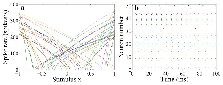
a. 1D tuning curves of a population of 50 leaky integrate-and-fire neurons. The maximum firing rate and x-intercept are chosen from uniform distributions with range 200Hz to 400Hz and −1 to +1, respectively. b. The neurons’ spike responses to a stimulus x = 0.5 (same color code).

IV. Kalman Filter with Spiking Neurons

To implement the Kalman filter with a SNN by applying the Neural Engineering Framework (NEF), we first convert (3) from discrete time (DT) to continuous time (CT), then we replace the CT matrices with neurally plausible ones, and use them to specify the SNN’s weights (Fig. 2). This yields:

$$\mathbf{x}(t)=h(t)\ast ({\mathbf{A}}^{\prime }\mathbf{x}(t)+{\mathbf{B}}^{\prime }\mathbf{y}(t)),$$ (7)

where

Fig. 2.

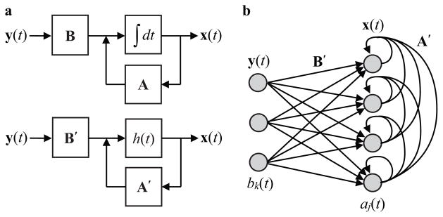
Implementing a Kalman filter with spiking neurons. a. Original Kalman filter (top) and neurally plausible version (bottom). The integrator is replaced with the synapses’ spike response, h(t), and the matrices are replaced with A′ = τA + I and B′ = τB to compensate. b. Spiking neural network implementation with populations b_k (t) and a_j (t) representing y(t) and x(t), respectively, and with feedforward and recurrent weights determined by B′ and A′, respectively.

$${\mathbf{A}}^{\prime }=\tau {\mathbf{M}}_x^{\text{CT}}+\mathbf{I}=\frac{\tau }{\mathrm{\Delta }t}({\mathbf{M}}_x^{\text{DT}}-\mathbf{I})+\mathbf{I},$$ (8)

$${\mathbf{B}}^{\prime }=\tau {\mathbf{M}}_y^{\text{CT}}=\frac{\tau }{\mathrm{\Delta }t}{\mathbf{M}}_y^{\text{DT}}.$$ (9)

${\mathbf{M}}_x^{\text{DT}}=(\mathbf{I}-\mathbf{KC})\mathbf{A}$ and ${\mathbf{M}}_y^{\text{DT}}=\mathbf{K}$ are the Kalman matrices, Δt is the discrete time step (50ms), and τ is the synaptic time constant.

The j^th neuron’s input current (see (6)) is computed from the system’s current state, x(t), which is computed from estimates of the system’s previous state ( $\widehat{\mathbf{x}}(t)={\sum }_i{a}_i(t){\phi }_i^{\mathbf{x}}$) and current input ( $\widehat{\mathbf{y}}(t)={\sum }_k{b}_k(t){\phi }_i^{\mathbf{y}}$) using (7). This yields:

$$\begin{array}{l}{\alpha }_j\langle {\stackrel{\sim }{\phi }}_j^{\mathbf{x}}·\mathbf{x}(t)\rangle +J_{\text{j}}^{\text{bias}}={\alpha }_j\langle {\stackrel{\sim }{\phi }}_j^{\mathbf{x}}·h(t)\ast ({\mathbf{A}}^{\prime }\widehat{\mathbf{x}}(t)+{\mathbf{B}}^{\prime }\widehat{\mathbf{y}}(t))\rangle +J_j^{\text{bias}}\\ ={\alpha }_j\langle {\stackrel{\sim }{\phi }}_j^{\mathbf{x}}·h(t)\ast \left({\mathbf{A}}^{\prime }\sum _i{a}_i(t){\phi }_i^{\mathbf{x}}+{\mathbf{B}}^{\prime }\sum _k{b}_k(t){\phi }_k^{\mathbf{y}}\right)\rangle +\dots \\ =h(t)\ast \left(\sum _i{\omega }_{ji}{a}_i(t)+\sum _k{\omega }_{jk}{b}_k(t)\right)+J_j^{\text{bias}}\end{array}$$ (10)

where ${\omega }_{ji}={\alpha }_j\langle {\stackrel{\sim }{\phi }}_j^{\mathbf{x}}{\mathbf{A}}^{\prime }{\phi }_i^{\mathbf{x}}\rangle$ and ${\omega }_{jk}={\alpha }_j\langle {\stackrel{\sim }{\phi }}_j^{\mathbf{x}}{\mathbf{B}}^{\prime }{\phi }_k^{\mathbf{y}}\rangle$ are the recurrent and feedforward weights, respectively.

V. Results

An adult male rhesus macaque (monkey L) was trained to perform variants of a point-to-point arm movement task in a 3D experimental apparatus for juice reward [1].¹ A 96-electrode silicon array (Blackrock Microsystems) was then implanted in premotor/motor cortex. Array recordings (−4.5 RMS threshold crossing applied to each electrode’s signal) yielded tuned activity for the direction and speed of arm movements. As detailed in [1], a standard Kalman filter model was fit by correlating the observed hand kinematics with the simultaneously measured neural signals, while the monkey was performing the point-to-point reaching task (Fig. 3). The resulting model was used online to control an on-screen cursor in real time. This model and 500 of these trials (2010-03-08) serves as the standard against which the SNN implementation’s performance is compared.

Fig. 3.

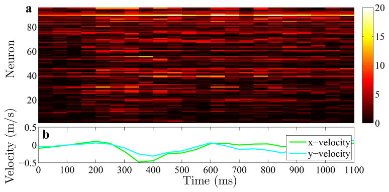
Neural and kinematic measurements for one trial. a. The ninety-six cortical recordings that were fed as input to the Kalman filter and the spiking neural network (spike counts in 50ms bins). b. Arm x- and y-velocity measurements that were correlated with the neural data to obtain the Kalman filter’s matrices, which were also used to engineer the neural network.

Starting with the matrices obtained by correlating the observed hand kinematics with the simultaneously measured neural signals, we built a SNN using the NEF methodology and simulated it in Nengo using the parameter values listed in Table I. We ensured that the time constants ${\tau }_i^{\text{RC}},{\tau }_i^{\text{ref}}$, and ${\tau }_i^{\text{PSC}}$ were smaller than the implementation’s time step (50ms).

TABLE I.

Model parameters

Symbol	Range	Description
max G(Jj (x))	200–400 Hz	Maximum firing rate
G(Jj (x)) = 0	−1 to 1	Normalized x-axis intercept
$J_j^{\text{bias}}$	Satisfies first two	Bias current
αj	Satisfies first two	Gain factor
${\stackrel{\sim }{\phi }}_j^{\mathbf{x}}$	$\Vert {\stackrel{\sim }{\phi }}_j^{\mathbf{x}}\Vert =1$	Preferred-direction vector
${\tau }_j^{\text{RC}}$	20 ms	RC time constant
${\tau }_j^{\text{ref}}$	1 ms	Refractory period
${\tau }_j^{\text{PSC}}$	20 ms	PSC time constant

We had the choice of two network architectures for the a_j(t) units: a single 3D integrator or two 1D integrators (Fig. 4). The latter were more stable, as reported previously [14], and yielded better results given the available computer resources. We also had the choice of representing the 96 neural measurements with the b_k(t) units (see Fig. 2b) or simply replacing these units’ spike rates with the measurements (spike counts in 50ms bins). The latter was more straight forward, avoided error in estimating the measurements, and conserved computer resources. Replacing b_k(t) with y(t)’s k^th component is equivalent to choosing ${\phi }_k^{\mathbf{y}}$ from a standard basis (i.e., a unit vector with 1 at the k^th position and 0 everywhere else), which is what we did.

Fig. 4.

Spiking neural network architectures. a. 3D integrator: A single population represents three scalar quantities—x and y-velocity and a constant. b. 1D integrators: A separate population represents each scalar quantity—x or y-velocity in this case.

The SNN performed better as we increased the number of neurons (Fig. 5a,b). For 20,000 neurons, the x and y-velocity decoded from its two 10,000-neuron populations matched the standard decoder’s prediction to within 0.03% (RMS error normalized by maximum velocity).² As reported in [10], the RMS error was roughly inversely proportional to the square-root of the number of neurons (Fig. 5c,d). There is a tradeoff between accuracy and computational time. For real-time operation—on a 3GHz PC with a 1ms simulation time-step—the network size is limited to 1,600 neurons. Encouragingly, this small network’s error was only 0.27%.

Fig. 5.

Comparing the x and y-velocity estimates decoded from 96 recorded cortical spike trains (10s of data) by the standard Kalman filter (blue) and the SNN (red). a,b. Networks with 2,000 and 20,000 spiking neurons. c. Dependence of RMS error (between SNN and Kalman filter) on network size (note log scale). d. Product of RMS error and neuron count’s (NC) square root is roughly constant (for NC > 200), implying that they are inversely proportional.

VI. Conclusions and Future Work

The Nengo simulations reported here demonstrate offline output that is virtually ident ical to that produced by a standard Kalman filter implementation. A 1,600-neuron network’s output is within 0.3% of the standard implementation, and Nengo can simulate this network in real-time. Which means we can now proceed to testing our new SNN on-line. This more challenging setting will enable us to further advance the SNN implementation by incorporating recently proposed variants of the Kalman filter that have been demonstrated to further increase performance and robustness during closed-loop, real-time operation [2], [3]. As such a filter and its variants have demonstrated the highest levels of brain-machine interface performance in both human [5] and monkey users [2], these simulations provide confidence that similar levels of performance can be attained with a neuromorphic architecture. Having refined the SNN architecture, we will proceed to our final validation step: implementing the network on Neurogrid, a hardware platform with sixteen programmable neuromorphic chips that can simulate a million spiking neurons in real-time [8].

The ultimate goal of this work is to build a fully implantable and programmable decoder chip using the neuromorphic approach. Variability among the silicon neurons and the large number of synaptic connections required present challenges. A distribution of spike-rates with a CV of 15% (sigma/mean) is typical, due to pronounced transistor mismatch in the subthreshold region where these nanopower circuits operate [9]. We have shown, however, that the NEF can effectively exploit even higher degrees of variability. Thus, the only real remaining challenge is achieving a high degree of connectivity. This one can be addressed by adopting a columnar organization, whereby nearby neurons share the same inputs, just like they do in the cortex—and in Neurogrid. This solution requires extending the NEF to a columnar architecture, a subject of ongoing research.

References

- 1.Gilja V. PhD Thesis. Department of Computer Science, Stanford University; 2010. Towards clinically viable neural prosthetic systems; pp. 19–22.pp. 57–73. [Google Scholar]
- 2.Gilja V, Nuyujukian P, Chestek CA, Cunningham JP, Fan JM, Yu BM, Ryu SI, Shenoy KV. 2010 Neuroscience Meeting Planner. San Diego, CA: Society for Neuroscience; 2010. A high-performance continuous cortically-controlled prosthesis enabled by feedback control design. [Google Scholar]
- 3.Nuyujukian P, Gilja V, Chestek CA, Cunningham JP, Fan JM, Yu BM, Ryu SI, Shenoy KV. 2010 Neuroscience Meeting Planner. San Diego, CA: Society for Neuroscience; 2010. Generalization and robustness of a continuous cortically-controlled prosthesis enabled by feedback control design. [Google Scholar]
- 4.Gilja V, Chestek CA, Diester I, Henderson JM, Deisseroth K, Shenoy KV. Challenges and opportunities for next-generation intra-cortically based neural prostheses. IEEE TBME. 2011 doi: 10.1109/TBME.2011.2107553. in press. [DOI] [PMC free article] [PubMed] [Google Scholar]
- 5.Kim SP, Simeral JD, Hochberg LR, Donoghue JP, Black MJ. Neural control of computer cursor velocity by decoding motor cortical spiking activity in humans with tetraplegia. J Neural Engineering. 2008;5:455–476. doi: 10.1088/1741-2560/5/4/010. [DOI] [PMC free article] [PubMed] [Google Scholar]
- 6.Kim S, Tathireddy P, Normann RA, Solzbacher F. Thermal impact of an active 3-D microelectrode array implanted in the brain. IEEE TNSRE. 2007;15:493–501. doi: 10.1109/TNSRE.2007.908429. [DOI] [PubMed] [Google Scholar]
- 7.Boahen K. Neuromorphic Microchips. Scientific American. 2005;292(5):56–63. doi: 10.1038/scientificamerican0505-56. [DOI] [PubMed] [Google Scholar]
- 8.Silver R, Boahen K, Grillner S, Kopell N, Olsen KL. Neurotech for neuroscience: Unifying concepts, organizing principles, and emerging tools. Journal of Neuroscience. 2007;27(44):11807–11819. doi: 10.1523/JNEUROSCI.3575-07.2007. [DOI] [PMC free article] [PubMed] [Google Scholar]
- 9.Arthur JV, Boahen K. Silicon Neuron Design: The Dynamical Systems Approach. IEEE Transactions on Circuits and Systems. doi: 10.1109/TCSI.2010.2089556. In press. [DOI] [PMC free article] [PubMed] [Google Scholar]
- 10.Eliasmith C, Anderson CH. Neural Engineering: Computation, representation, and dynamics in neurobiological systems. MIT Press; Cambridge, MA: 2003. [Google Scholar]
- 11.Kalman RE. A New Approach to Linear Filtering and Prediction Problems. Transactions of the ASME–Journal of Basic Engineering. 1960;82(Series D):35–45. [Google Scholar]
- 12.Welsh G, Bishop G. An Introduction to the Kalman Filter. TR 95-041. Vol. 95. University of North Carolina; Chapel Hill Chapel Hill NC: 1995. pp. 1–16. [Google Scholar]
- 13.Eliasmith C. A unified approach to building and controlling spiking attractor networks. Neural Computation. 2005;17:1276–1314. doi: 10.1162/0899766053630332. [DOI] [PubMed] [Google Scholar]
- 14.Singh R, Eliasmith C. Higher-dimensional neurons explain the tuning and dynamics of working memory cells. The Journal of Neuroscience. 2006;26(14):3667–3678. doi: 10.1523/JNEUROSCI.4864-05.2006. [DOI] [PMC free article] [PubMed] [Google Scholar]
- 15.Eliasmith C. How to build a brain: from function to implementation. Synthese. 2007;159(3):373–388. [Google Scholar]