Humans make efficient use of natural image statistics when performing spatial interpolation

Abstract

Visual systems learn through evolution and experience over the lifespan to exploit the statistical structure of natural images when performing visual tasks. Understanding which aspects of this statistical structure are incorporated into the human nervous system is a fundamental goal in vision science. To address this goal, we measured human ability to estimate the intensity of missing image pixels in natural images. Human estimation accuracy is compared with various simple heuristics (e.g., local mean) and with optimal observers that have nearly complete knowledge of the local statistical structure of natural images. Human estimates are more accurate than those of simple heuristics, and they match the performance of an optimal observer that knows the local statistical structure of relative intensities (contrasts). This optimal observer predicts the detailed pattern of human estimation errors and hence the results place strong constraints on the underlying neural mechanisms. However, humans do not reach the performance of an optimal observer that knows the local statistical structure of the absolute intensities, which reflect both local relative intensities and local mean intensity. As predicted from a statistical analysis of natural images, human estimation accuracy is negligibly improved by expanding the context from a local patch to the whole image. Our results demonstrate that the human visual system exploits efficiently the statistical structure of natural images.

Introduction

Visual systems evolve and develop with natural images as input. Natural images are highly structured statistically, and thus visual systems are likely to exploit this statistical structure when encoding the retinal images and performing visual tasks (Barlow, 1961; Brunswik & Kamiya, 1953; Field, 1987; Kersten, 1987; Laughlin, 1981; Maloney, 1986; for reviews see Geisler, 2008; Simoncelli & Olshausen, 2001).

Much of the work concerning natural image statistics has been directed at measuring the statistical structure of images and performing theoretical analyses of how best to exploit that structure (Geisler, 2008; Simoncelli & Olshausen, 2001). Less common have been attempts to determine experimentally how visual systems actually do exploit the structure of natural images when performing visual tasks (Burge, Fowlkes, & Banks, 2010; Fine, MacLeod, & Boynton, 2003; Freeman, Ziemba, Heeger, Simoncelli, & Movshon, 2013; Geisler & Perry, 2009; Geisler, Perry, Super, & Gallogly, 2001; Gerhard, Wichmann, & Bethge, 2013; Ing, Wilson, & Geisler, 2010; Kersten, 1987; Laughlin, 1981.

Kersten (1987) carried out a clever early study. Pixels were removed from natural images and subjects were required to estimate the gray level of the missing pixels. An important feature of this task is that it provides a precise quantitative measure of what the human visual system understands about the local statistical structure of natural images—the more accurate the estimated gray levels (given the local image context), the better the understanding. This task is also an interesting special case of image interpolation, which is a ubiquitous natural task. For example, projection of the three-dimensional (3-D) scene onto the two-dimensional (2-D) retina causes many occlusions, across which the visual system must interpolate (Albright & Stoner, 2002; Field, Hayes, & Hess, 1993; Kellman & Shipley, 1991; Singh & Fulvio, 2005). Interpolation also arises in filling in the blind spot and angioscotomas, and in estimating the stimulus between the image samples taken by the photoreceptors (Brainard & Williams, 1993; Williams, MacLeod, & Hayhoe, 1981).

In Kersten's (1987) study, subjects guessed the gray level repeatedly (with feedback) until they guessed the true value (this is a version of Shannon's guessing game). The aim was to obtain a lower bound on the redundancy of natural images and to compare human guesses with some simple nearest-neighbor interpolation algorithms. This experimental procedure for measuring image redundancy requires that subjects can clearly discriminate each gray level and hence it was necessary to quantize the images to 16 gray levels (4 bits). For a version of the guessing game that does not require quantized gray levels, see Bethge, Wiecki, and Wichmann (2007).

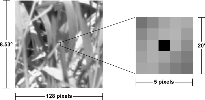
Here, we use a modified version of Kersten's (1987) pixel estimation task to address a different aim. In recent work, we measured the statistical structure of images relevant for the task of estimating missing pixel values in full 256 gray level (8 bit) natural images (Geisler & Perry, 2011). The present aim is to determine to what extent the human visual system has incorporated these statistical regularities. Specifically, we measure psychometric functions (without feedback), where the observer judges whether the gray level of the missing pixel is too bright or too dim given the image context (see Figure 1). We then take the 50% point of the psychometric function to be the observer's gray-level estimate.

Figure 1.

Pixel estimation task. The task is to estimate the gray level of the central 4′ wide pixel (black pixel) of a natural image patch, given the context of the surrounding image. Estimates were taken to be the 50% point of psychometric functions where the observer reported on each trial whether the central pixel was too bright or too dim. No feedback was given. Estimates were measured given the full (128 × 128) context and given a restricted (5 × 5) context. The contexts were surrounded by the mean gray level of the full image.

We find that human estimates are better than those of simple models such as the mean or median of the local contextual pixels. Instead we find that humans make near optimal use of the local spatial statistics of natural images. Remarkably, the specific pattern of human estimation errors across image patches closely matches those of a model observer that optimally exploits the local statistical structure of relative intensities (contrasts) in natural images.

Model observers

In the pixel estimation task the central pixel of an image patch is removed and the goal is to estimate the gray level of the missing pixel given the surrounding context of pixel values. We consider a variety of model observers for this task.

First consider an observer that approximates the Bayesian ideal observer. Let z represent the true (unknown) value of the missing pixel, and the c represent the context of surrounding pixel values. The optimal estimate is given by the standard formula from Bayesian statistical decision theory:

where γ(z, ẑ) is the cost of making the estimate ẑ when the true value is z, and p(z|c) is the posterior probability that the true value is z given the observed context. For present purposes we assume the cost function is the squared error between the true value and the estimated value, γ(z, ẑ) = (z − ẑ)². For this cost function it is well known (e.g., Bishop, 2006) that the optimal estimate is the conditional mean of the posterior probability distribution (the so-called minimum mean squared error [MMSE] estimate):

Thus, determining the Bayesian ideal observer reduces to determining the conditional mean for each possible set of context values. In general, this is extremely difficult because of the enormous number of possible combinations of context values. However, in this particular case statistical analysis suggests that the relevant context pixels are only those spatially near to the missing pixel, and thus a simple and powerful approach is to directly estimate conditional means for several small contexts and then combine those estimates using the relative reliability of the estimates. Specifically, in a previous study (Geisler & Perry, 2011) we directly estimated conditional means from a large collection of calibrated natural images for context vectors consisting of the four pixels in line with the missing pixel (in either the vertical or horizontal direction), and then combined the vertical and horizontal estimates based on their relative reliabilities. Formally, the context vector for the horizontal direction, for a pixel at location (x, y), was c = [z(x – 2, y), z(x – 1, y), z(x + 1, y), z(x + 2, y)] and the context vector in the vertical direction was c^⊥ = [z(x, y – 2), z(x, y – 1), z(x, y + 1), z(x, y + 2)]. The optimal estimates for these two contexts are ẑ_opt = E(z|c) and = E(z|c^⊥), and the combined estimate is given by

where ρ_opt = 1/Var(z|c), = 1/Var(z|c^⊥), ρ = 1/Var(z), and u = E(z). Equation 3 specifies the Bayesian optimal combination rule when two contexts (c and c^⊥), conditioned on the true value z(x, y), are statistically independent and Gaussian distributed. When the variance of the prior is infinite (ρ = 0), then Equation 3 reduces to the standard cue combination formula (Oruc, Maloney, & Landy, 2003).

Although not proven, our previous results suggest that the estimates obtained using the horizontal and vertical contexts, with the above combination rule, are near optimal (Geisler & Perry, 2011). We will refer to this model observer as the LumOpt8 observer, since it uses eight luminance (gray-level) values. We also consider the LumOpt4 observer that uses only the neighboring two luminance values in each direction.

It is well known that visual neurons beyond the photoreceptors and horizontal cells are often better described as encoding contrast rather than luminance. Thus, it is reasonable to consider a Bayesian ideal observer that operates on contrast images rather than luminance images. Here, we define the contrast image by

where ẑ(x, y) is the average value of z in the 3 × 3 neighborhood centered on (x, y). The ConOpt8 and ConOpt4 observers are defined exactly as above, but for contrast images rather than luminance images. Thus, the context vectors now consist of the contrast-image values. We note that the local statistical structure of natural images changes with the local mean luminance, and hence estimates based on the statistics of contrast images will generally be less accurate than those based on the statistics of luminance images (see Geisler & Perry, 2011).

To obtain the gray levels estimated by these contrast observers, the gray level of the center pixel (z) was varied from 0 to 255. At each gray value of the center pixel, we calculated the contrast of the center pixel z_C as well as the optimal prediction of the contrast at the central pixel using the context. Note that as z is varied, the values of the context vectors may also vary because the local average, ẑ(x, y), for some context pixels includes the center pixel being estimated. The gray level of the central pixel at which z_C most nearly equals is the gray level prediction of the model contrast observers.

Combining estimates with relative reliability (Equation 3) assumes that the two estimates are statistically independent and Gaussian, given the true gray level of the missing pixel. While Equation 3 works well for the LumOpt8 observer, we find that ConOpt8 and ConOpt4 performance is slightly better when the two estimates are averaged rather than combined with relative reliability. Below we report the performance of the contrast observers based on averaging.

We also considered model observers based on multiple linear regression: LumMlr8 and ConMlr8 (least squares linear estimators based on the same eight pixels as LumOpt8 and ConOpt8), and LumMlr4 and ConMlr4 (least squares linear estimators based on the same four pixels as LumOpt4 and ConOpt4). These linear models were also trained on the natural images. Finally, we considered several simpler model observers: Mean8 (the average of the surrounding eight pixels), Mean24 (the average of the surrounding 24 pixels), Median4 (median of the four nearest pixels), Median8 (the median of the surrounding eight pixels), and Median24 (the median of the surrounding 24 pixels). We also consider a NoContext observer, which has no knowledge of the spatial context of the central pixel, and therefore uses only the prior on gray levels in natural images to estimate the missing pixel value.

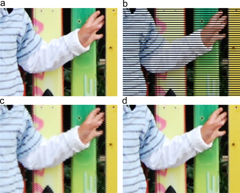
The difference in estimation accuracy between using the local mean and using the local statistics of natural images is illustrated in Figure 2. In this demonstration we removed every third horizontal row of pixels from an original image (Figure 2b) and then estimated those pixels using the local mean (Figure 2c) and the local luminance statistics (Figure 2d). Using the local mean produces substantial artifacts, whereas using the local luminance statistics produces no noticeable artifacts and the image appears very similar to the original (Figure 2a). This example demonstrates the potential value of exploiting natural image statistics. Detailed quantitative comparisons of model observers and human observers are given below.

Figure 2.

Demonstration of model-observer estimates. (a) Original image. (b) Every third row of pixels is removed from an original image. (c) Pixels estimated using local mean (notice artifacts near edges). (d) Pixels estimated using local statistics of natural images. The different color channels were processed independently and identically.

Methods

Subjects

Three observers performed the experiments. All had corrected-to-normal vision. One observer was an author, and the other two were naive to the purpose of the experiment.

Stimuli

Stimuli were presented on a Sony GDM-F520 cathode ray tube (CRT) display (Sony Corporation, Tokyo, Japan) with a 1600 × 1200 pixel resolution, at a frame rate of 60 Hz. The display was linearized over 8 bits of gray level. The maximum luminance was 104.3 cd/m². Each image pixel in the presented patches had a visual angle of 4 arc min (4 × 4 display pixels). This size was picked so that the individual test pixel was clearly visible, yet the image appeared relatively smooth and continuous.

The test stimuli consisted of 62 natural image patches (128 × 128 pixels, 8-bit grayscale) sampled from a set of 415 images (each 4284 × 2844 pixels). Raw color 14-bit images were collected using a calibrated Nikon D700 camera (Nikon Corporation, Tokyo, Japan). The images were taken in the Austin area, and contained no human-made objects. The camera was set to a low ISO setting of 200 (which minimizes camera noise), and care was taken to minimize clipping. The raw images were converted to YUV space. To obtain the test images, the Y values were scaled and quantized to 8 bits such that the top 2% of the pixels had a value of 255. More details and the images are available at http://www.cps.utexas.edu/natural_scenes/db.shtml.

The specific image patches were selected to span the range of local contexts that occur in natural images. If image patches are randomly sampled, then they tend to be dominated by cases where the central pixel is similar in gray level to the contextual pixels. For such patches, pixel estimation is relatively easy and all models perform nearly equally well. By spanning the range of local contexts we are able to better distinguish between different models.

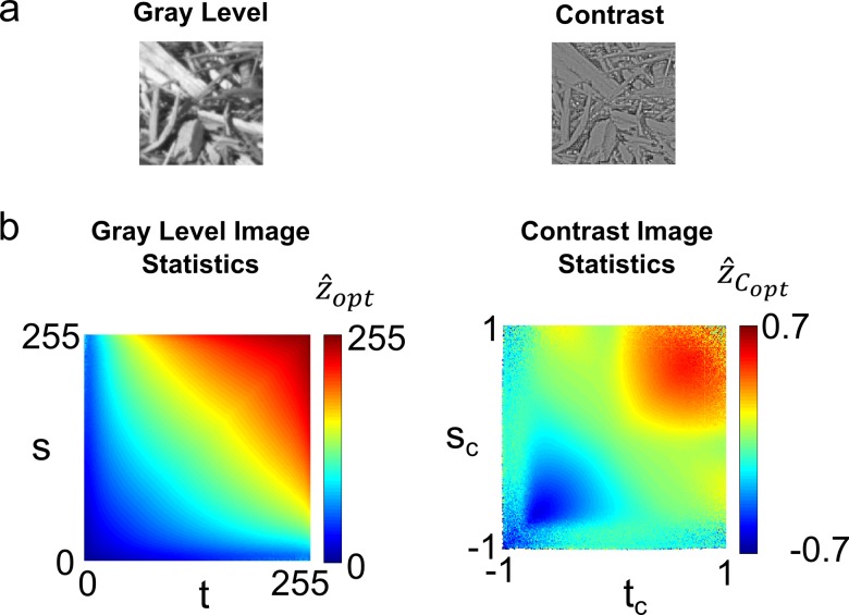
To span the range of contexts we examined the local gray level statistics in natural scenes. The left plot in Figure 3b shows the optimal estimates, ẑ_opt, for the missing pixel z(x, y) given the two neighboring horizontal pixels, z(x − 1, y), z(x + 1, y). In the figure, s and t represent the neighboring pixels' values. The horizontal and vertical axes give the 8-bit gray values of s and t and the color scale gives the optimal estimate. As expected, swapping the values of s and t does not change the optimal estimate, and hence the plot is symmetric about the diagonal.

Figure 3.

Local spatial statistics of natural gray-scale and contrast images. (a) The expected gray-scale value of a natural image pixel ẑ_opt given the values of the neighboring pixels (s, t) in the horizontal or vertical direction. (b) The expected Weber-contrast value of a natural image pixel ẑ_Copt given the values of the neighboring pixels (s_C, t_C) in the horizontal or vertical direction.

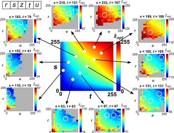
If the optimal estimate were always the average of s and t, then the contours of constant color in this plot would be straight lines with a slope of −1.0 (Geisler & Perry, 2011). As can be seen, there are substantial systematic deviations from the simple average, and the deviations are in different directions in different regions of s-t space. Therefore, it is important to sample from the different regions of the space. At the same time, we want to sample from regions of the space that are not extremely rare. The white points in the central plot of Figure 4 show the values of s and t from which the samples were drawn. The values of s and t along the diagonal are the pairs that occur most frequently. The values of s and t that are off the diagonal occur less frequently than those along the diagonal, but with equal frequency to one another.

Figure 4.

Selection of test patches. Test patches were selected to span the range of local contexts that occur in natural images. The white closed circles in the central plot show the values of s and t that were tested. For each of these values of s and t, the outer plots show the expected value (optimal estimate) of the central pixel (ẑ_opt) given the values of r, s, t, and u. Notice that for each particular pair of values of s and t, the optimal estimate is strongly modulated by the values of r and u. The white open circles show the locations in (r, s, t, u) space from which the test patches were selected—two patches were randomly selected from the patches falling within each white circle.

The white closed circles in the central plot specify values of context pixels immediately adjacent to the missing pixel. Those pixel values are shown at the tops of the outer plots. The color scale in the outer plots shows the optimal estimates (conditional means) given all four context values (r, s, t, u). These plots show that for fixed values of s and t, the optimal estimate can vary dramatically, depending on the specific values of the more distant pixels r and u. Therefore, to tile the range of natural image patches, and to test whether the visual system incorporates the statistical structure revealed in Figure 4, we selected patches whose values of r, s, t, and u fell within the open circles of the outer plots. Two patches were randomly selected from each circle.

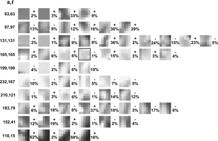
The central 5 × 5 regions of the 62 selected patches are shown in Figure 5. As might be expected, there is substantial variety among the selected patches; there are patches with different lightness, patches with horizontal, vertical, and diagonal edges, patches with vertical, horizontal, and diagonal bars, patches with central spots, etc. This suggests that we succeeded in selecting a set of stimuli that is representative of the variety that occurs in natural images.

Figure 5.

Test image patches. Shown are the 5 × 5 test patches that were randomly sampled from the regions of (r, s, t, u) space given in Figure 4 (white circles in Figure 4). The numbers to the right of each patch give the percent error of the human estimate from the true value of the center pixel. The black box indicates the test patch for the psychometric functions shown in Figure 5a.

Procedure

Psychometric functions were measured for the 62 full 128 × 128 pixel patches and for the same patches cropped to the central 5 × 5 pixels. The surrounding gray level for both 5 × 5 and 128 × 128 patches was the same as the overall mean gray level of the image from which the patch was taken.

Seven point psychometric functions were measured using the method of constant stimuli. The seven gray levels for the central pixel were determined in a preliminary experiment, and the same gray levels were used for 128 × 128 and 5 × 5 patches. All patches and central pixel gray levels were presented once, in a random order, in each experimental session. There were 30 sessions. Thus each value at the seven levels of the psychometric functions was based on 30 measurements (210 measurements per psychometric function).

The observer's head was stabilized via a chin rest while viewing the monitor screen from a distance of 74 cm. At the start of a trial, the central pixel of the patch blinked from black to white for 1 s to indicate its location. Then one of the seven gray levels was presented. The observer indicated whether they thought the gray level of the central pixel was brighter or darker than the true gray level in the patch. If the observer became unsure of the location of the central pixel, they could press a button that would cause it to blink again for 1 s. The observer had unlimited viewing time to perform each judgment. No feedback was given. After the observer indicated their judgment, the screen became uniform gray for 1 s, and then the next random stimulus was selected and the process repeated.

The psychometric data were fit with a cumulative Gaussian function using a maximum likelihood procedure. Confidence intervals on the mean and standard deviation of the cumulative Gaussian fits were calculated by bootstrapping. On each trial, each point on the psychometric function was randomly drawn from a binomial distribution with p given by the measured value (proportion of “brighter” responses) at that level, and n equal to 30. These randomly drawn points were then refit with a cumulative Gaussian using a maximum likelihood procedure. This was repeated 10,000 times, and the resulting distributions for the mean and standard deviation of the cumulative Gaussian were used to generate 95% confidence intervals (±2σ).

Results

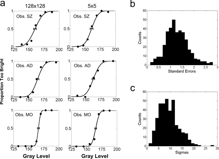
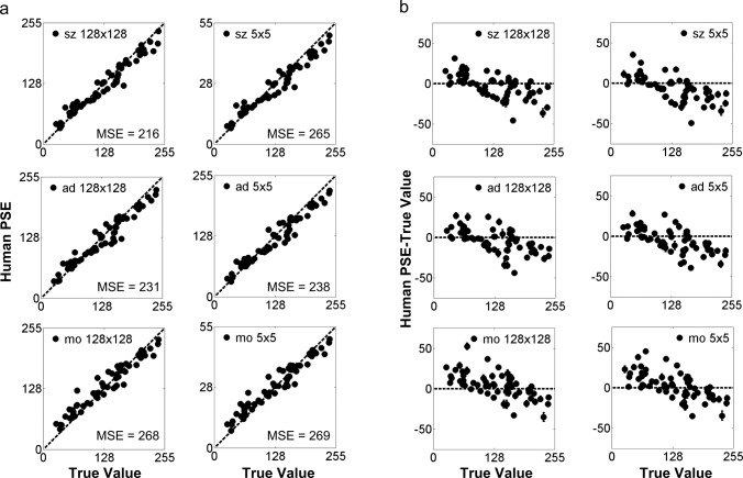
Example psychometric functions for the three observers and both patch sizes are shown in Figure 6a (the specific patch is indicated by the black box in Figure 5). The standard errors of the point of subjective equality (PSE) estimates were very small (an average of 1.38 gray level steps out of 255; Figure 6b), and hence the estimates are quite reliable. The observers' estimates (PSEs) for all of the 5 × 5 and 128 × 128 patches are plotted in Figure 7a as a function of the true gray level. If observers' estimates perfectly predicted the true gray levels, then the data points would lie on the dashed line. Observers' PSEs follow the dashed line fairly closely, showing that human observers are quite accurate at estimating the true value of a missing pixel.

Figure 6.

Human pixel estimation psychometric functions. (a) Psychometric functions for three observers and two context sizes, for the image patch indicated with the black box in Figure 5. Human estimates (PSEs) were taken to be the 50% point of the psychometric functions, which were fitted with a Gaussian integral function. Error bars indicate 95% confidence intervals of the 50% point. (b) Histogram of standard errors for the PSEs for all 372 psychometric functions (3 observers × 2 context sizes × 62 patches). (c) Histogram of the sigmas of the fitted cumulative Gaussians for all 372 psychometric functions. The average sigma is 9.32. The average sigma in (a) is 7.62.

Figure 7.

Human pixel estimation accuracy. (a) Performance accuracy for all conditions for all observers. The horizontal axis is the actual gray level of the missing pixel and the vertical axis is the value estimated by the human observers. If performance were perfect all points would fall along the diagonal line. Also, given is the MSE of the human estimates. (Note that these MSE values correspond to standard deviations of around 15 to 16 gray-level steps.) (b) Human estimation errors for all conditions and observers. The horizontal axis is the actual gray level of the missing pixel and the vertical axis is the difference between the observer's estimate and the actual gray level of the missing pixel.

On the other hand, there are clear systematic differences between the human estimates and the true values. This is illustrated in Figure 7b, which plots the estimation errors as a function of the true value. Roughly speaking, the observers tended to overestimate low true values and underestimate high true values. Overall, the observers tended to underestimate the gray value. Finally, notice that the specific pattern of errors in Figure 7b is similar across the three observers and across the two patch sizes.

To quantify these differences we computed the MSE between the estimated and true values:

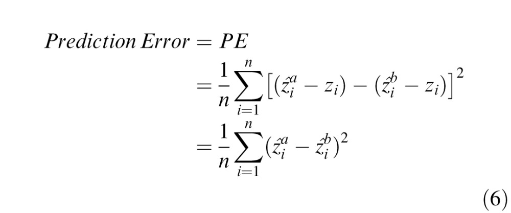
The MSEs are given in Figure 7a. Interestingly, the human estimation accuracy is only slightly better for the full 128 × 128 context than for the 5 × 5 context (an average MSE of 238 vs. 257). Also, the specific pattern of errors, across patches, made by the three observers is very similar. To quantify the similarity in the pattern of errors we compute the MSE between the observers' errors, which is equivalent to the mean square error between their estimates:

where and are the estimates by two observers for the i^th patch. The average prediction error (PE) between pairs of observers is 87, which is small relative to their MSEs. In other words, the error between observers' estimates is much smaller than the error between the observers' estimates and the true values.

The numbers to the right of each test patch in Figure 5 show the sign and magnitude of the human errors (averaged over the three observers and patch sizes), expressed as a percentage of the ground truth gray value of the center pixel. Although the pattern of errors is complex, the errors tend to be smallest when the gray levels of the pixels near the center pixel are similar to each other and to the center pixel.

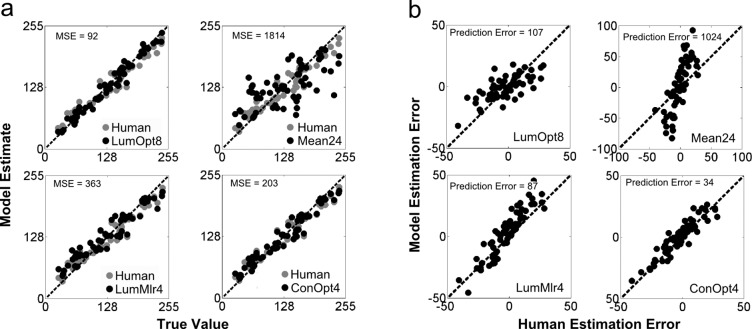
How do the human estimates compare with those of the various model observers? Given that human performance was similar across the three observers and patch sizes, we compared model predictions with the average performance across the three observers and patch sizes. These average human estimates (gray circles) are shown along with the predictions of four different models (black circles) in Figure 8a. The MSEs of the model observers are shown in the upper left corner of each plot. Again each plot in Figure 8a gives the estimated gray value as a function of the true value. The estimates of the LumOpt8 observer are substantially more accurate than those of the human observers (MSE = 92 vs. MSE = 215). This indicates that there is substantial statistical structure in natural images that the human visual system does not exploit efficiently. On the other hand the Mean24 observer performs far worse than humans (MSE = 1814 vs. MSE = 215). The multiple linear regression observer that uses the four nearest pixels (LumMlr4) also performs worse than humans (MSE = 363). The model that best matches overall human estimation accuracy is the ConOpt4 observer (MSE = 203). The natural image statistics upon which the ConOpt4 observer is based are shown in Figure 3b.

Figure 8.

Predictions of model observers. Human estimates have been averaged across observers and context size, and therefore are the same in every panel. (a) The black symbols show the gray level estimated by four of the model observers, as a function of the true gray level of the missing pixel. For reference, the gray symbols show the estimates made by the human observers. Note that human data are the same in every panel. The MSEs of the model observers' estimates are shown in the upper left corner of each panel. (b) Estimate errors of the four model observers, for each test patch, as a function of the human estimation error. If a model observer precisely predicted the human errors then all the points would fall along the positive diagonal. Also shown is the PE—the MSE between model and human estimates.

The MSEs for all the model observers (and human observers) are shown in the second column of Table 1. Also, the first row of the table shows the performance based on using only the prior probability of gray levels in natural images (i.e., not using the context at all). There are several points to make about the MSE values. First, the MSE of the LumOpt8 observer is much lower than that of the ConOpt8 observer. This implies that there is considerable useful information contained in the absolute gray levels that is not contained in the relative gray levels (see also Geisler & Perry, 2011). Second, the MSE of the LumOpt4 observer is higher than that of both the ConOpt8 and ConOpt4 observers, which are similar to each other. Presumably, this occurs because ConOpt4 observer's estimates incorporate pixel values over a larger area than the LumOpt4 observer. Third, the MSEs of the observers based on the local median and the mean are similar and much higher than the MSE of the human observers. The MSEs of the Median4 and LumMlr4 observers are similar. This is expected since LumMlr4 (in this case) is similar to the mean of the four nearest pixels. Fourth, the ConMlr observers perform better than the ConOpt observers. This unexpected result occurs because the model observers are optimized based on the entire training set of natural image patches. On both the training set and test set, which each consisted of many millions of patches, the ConOpt observers perform substantially better than the ConMlr observers. Thus, the reversal is only for the specific set of 62 patches in the experiment.

Table 1.

Model observer estimation error and prediction error. Note: MSE = mean squared error; PE = prediction error.

Observer	MSE	PE
NoContext	8,897	7,717
LumOpt8	92	107
LumOpt4	297	95
ConOpt8	164	48
ConOpt4	203	34
LumMlr8	111	144
LumMlr4	363	87
ConMlr8	129	57
ConMlr4	160	41
Mean24	1,811	1,024
Mean8	590	186
Median24	1,727	1,051
Median8	580	256
Median4	343	85
Human	215	—

More important than predictions of overall performance is the question of how well the models predict the specific estimation errors made by the human observers. Figure 8b plots the predicted estimation errors of four of the model observers as a function of the estimation error of the human observers, for all 62 test patches. If a model observer predicted the human estimates exactly, then the data points would fall along the dashed diagonal line. The average prediction error of each model is indicated in the figure. The prediction error of the ConOpt4 observer is the smallest (Table 1). Interestingly, the prediction error of all the ConOpt and ConMlr observers are substantially lower than the prediction error of the other models. This result suggests that for any randomly chosen natural image patch, the local contrast-image statistics of natural images predict (with good accuracy) both the magnitude and sign of human estimation errors in the pixel estimation task.

In addition to the model observers shown in Table 1 we also ran multiple linear regression models with a full 5 × 5 context (minus the center pixel). This model predicted human estimates less accurately than the contrast models in Table 1. Its estimates were 1% more accurate than the LumOpt8 observer on the 62 test patches (MSE = 91 vs. MSE = 92), but were 4% less accurate on five million randomly selected test patches (MSE = 14.51 vs. MSE = 13.97).

Discussion

A simple pixel interpolation task was used to assess how well the human visual system exploits the local structure of natural images. Sixty-two representative gray-level patches of natural image were selected. For each patch, psychometric functions were measured, where the task was to report (without feedback) whether the central pixel in the patch was too bright or too dim given the surrounding context of image pixels. The PSE was taken as the human estimate of gray level. The observers reported that the task was relatively easy, which was consistent with the fact that the estimates of the PSEs were reliable and similar across observers.

Although the human estimates are quite accurate, there are clear systematic deviations from the ground truth values. These deviations are very similar for the three observers. Further, the observers' estimates are nearly the same for 5 × 5 and 128 × 128 pixel patches, revealing that the visual system primarily uses the information in a local 5 × 5 pixel neighborhood to estimate missing points in an image. This result is consistent with the falloff of correlation in natural images (Deriugin, 1956; Field, 1987) and with our previous statistical analysis of natural image patches, which strongly suggests that the most informative pixels are the two on each side of the missing pixel in the vertical and horizontal directions (Geisler & Perry, 2011).

Human performance was compared with that of a number of model observers. Humans outperform simple model observers (local mean, local median), but do not reach the performance of an observer that makes near-optimal use of the local spatial statistics of natural luminance images. However, human performance closely matches that of an observer that makes optimal use of the local spatial statistics of natural contrast images (images where each pixel has been converted from a luminance value to a Weber contrast value). Apparently, the human visual system uses precise knowledge of local contrast-image statistics in the pixel estimation task.

A recent study also provides evidence for sophisticated mechanisms in very local estimation tasks. Hofer, Singer, and Williams (2005) used adaptive optics to stimulate individual cones and asked subjects to estimate the perceived color of the stimulus. They found that humans produce different color names from stimulation of the same type of cone, depending on the specific types of cones in the surrounding region. Subsequent statistical analysis, using the specific cone mosaics of the human observers, showed that in fact this complex pattern of estimates is consistent with a sophisticated Bayesian estimation mechanism (Brainard, Williams & Hofer 2008).

Kersten (1987) showed that performance for one human observer in the Shannon guessing task was very similar for 8-pixel and 1224-pixel contextual neighborhoods. A similar result is reported by Bethge et al. (2007). Kersten also blocked out the nearest 24 pixels and showed that performance dropped precipitously, but not to chance, indicating that humans can use more distant information. We have not carried out similar psychophysical tests, but we have carried out statistical analyses showing that there is predictive information in the more distant pixels; that information is simply dwarfed by the much better information in the nearby pixels. This is not a surprising result given the long-range correlations implied by the 1/f amplitude spectra of natural images (Deriugin, 1956; Field, 1987).

The present study (like the previous studies listed in the Introduction) demonstrates the value of measuring natural image statistics that are relevant for specific tasks. In particular, the measured contrast image statistics directly predict much of the human observers' estimation performance in the pixel estimation task. Furthermore, given that the test patches were selected to be generally representative of those in natural scenes, there is every reason to think that the measured image statistics would do a good job of predicting human performance for arbitrary natural image patches. This finding complements our previous study demonstrating that the statistics of contour shape in natural images predict human performance in a contour occlusion task where the observers' task is to estimate whether contour elements passing under an occluder belong to the same or different physical contours (Geisler & Perry, 2009).

The fact that human pixel estimation performance is accurately predicted by an observer that makes efficient use of the local spatial statistics of contrast images must place strong constraints on the underlying neural mechanisms. However, the constraints are not as strong as for the contour occlusion task. In the contour occlusion task, humans approach the best performance possible, and hence the detailed structure of the natural image contour statistics must be implemented implicitly (or explicitly) in the neural mechanisms. On the other hand, in the pixel estimation task, humans do not reach the best performance possible, which is that of the observer that makes optimal use of the local spatial statistics of luminance images. This gap leaves room for a wider range of neural mechanisms. For example, the human visual system could make suboptimal use of both the local luminance-image and contrast-image information. It is possible that such models predict performance as well as the contrast-image ideal. Nonetheless, it is quite remarkable that the specific errors that humans make can be so accurately predicted by natural image statistics.

Although the image statistics were obtained by measuring a very large number of conditional means (one mean for each configuration of context values), the statistics are smooth functions of the context values (see Figures 3 and 4). Thus, these functions may be implemented with relatively simple neural circuits that could have evolved or been learned during development. Indeed, the multiple linear regression models show that appropriate linear weights on the contrast image can predict human errors quite well. Figure 9 shows a simple ConMlr model (outside the family of models in Table 1) that predicts human errors slightly more accurately than the ConOpt4 model in Table 1.

Figure 9.

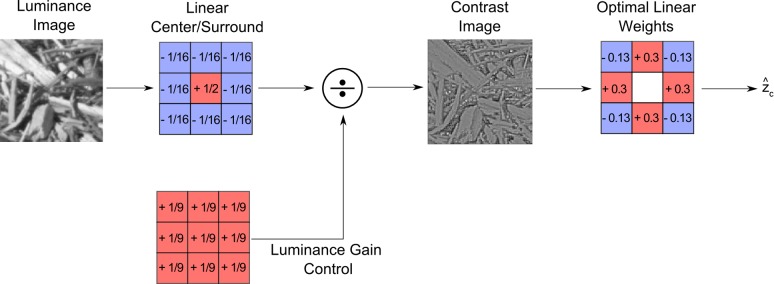
A simple model of missing pixel estimation in humans. The input image is passed through a center-surround linear filter and normalized by the local luminance, producing a Weber contrast response at each pixel location (similar to the response of a ganglion cell). The estimate of Weber contrast at the missing pixel is obtained by applying a fixed set of linear weights (shown on the right) to the eight pixel locations immediately surrounding the missing pixel. These weights were learned on a training set consisting of millions of randomly selected natural image patches.

Finally, the present pixel estimation task is subjectively easy, yielding precise estimates that are consistent across observers. Thus, this task is a promising tool that could be used to explore how the human visual system exploits both the luminance and chromatic structure of natural and artificial images.

References

- Albright T. D., Stoner G. R. (2002). Contextual influences on visual processing. Annual Review of Neuroscience, 25, 339–379 [DOI] [PubMed] [Google Scholar]
- Barlow H. B. (1961). The coding of sensory messages. In Thorpes W. H., Zangwill O. L. (Eds.), Current problems in animal behavior (pp 331–360) Cambridge, UK: Cambridge University Press; [Google Scholar]
- Bethge M., Wiecki T. V., Wichmann F. A. (2007). The independent components of natural images are perceptually dependent. Proceedings of SPIE Human Vision & Electronic Imaging XII, 6492, 1–12 [Google Scholar]
- Bishop C. M. (2006). Pattern recognition and machine learning. New York: Springer; [Google Scholar]
- Brainard D. H., Williams D. R. (1993). Spatial reconstruction of signals from short-wavelength cones. Vision Research, 33, 105–116 [DOI] [PubMed] [Google Scholar]
- Brainard D. H., Williams D. R., Hofer H. (2008). Trichromatic reconstruction from the interleaved cone mosaic: Bayesian model and the color appearance of small spots. Journal of Vision, 8 (5): 11 1–23, http://www.journalofvision.org/content/8/5/15, doi:10.1167/8.5.15 [Pubmed] [Article] [DOI] [PMC free article] [PubMed] [Google Scholar]
- Brunswik E., Kamiya J. (1953). Ecological cue-validity of “proximity” and of other Gestalt factors. American Journal of Psychology, 66, 20–32 [PubMed] [Google Scholar]
- Burge J., Fowlkes C. C., Banks M. S. (2010). Natural-scene statistics predict how the figure-ground cue of convexity affects human depth perception. Journal of Neuroscience, 30, 7269–7280 [DOI] [PMC free article] [PubMed] [Google Scholar]
- Deriugin N. (1956). The power spectrum and the correlation function of the television signal. Telecommunications, 1 (7), 1–12 [Google Scholar]
- Field D. J. (1987). Relations between the statistics of natural images and the response properties of cortical cells. Journal of the Optical Society of America, 4, 2379–2394 [DOI] [PubMed] [Google Scholar]
- Field D. J., Hayes A., Hess R. F. (1993). Contour integration by the human visual system: Evidence for a local association field. Vision Research, 23, 173–193 [DOI] [PubMed] [Google Scholar]
- Fine I., MacLeod D. I. A., Boynton G. M. (2003). Surface segmentation based on the luminance and color statistics of natural scenes. Journal of the Optical Society of America, 20, 1283–1291 [DOI] [PubMed] [Google Scholar]
- Freeman J., Ziemba C. M., Heeger D. J., Simoncelli E. P., Movshon J. A. (2013). A functional and perceptual signature of the second visual area in primates. Nature Neuroscience, 16, 974–981 [DOI] [PMC free article] [PubMed] [Google Scholar]
- Geisler W. S. (2008). Visual perception and the statistical properties of natural scenes. Annual Review of Psychology, 59, 167–192 [DOI] [PubMed] [Google Scholar]
- Geisler W. S., Perry J. S. (2009). Contour statistics in natural images: Grouping across occlusions. Visual Neuroscience, 26, 109–121 [DOI] [PMC free article] [PubMed] [Google Scholar]
- Geisler W. S., Perry J. S. (2011). Statistics for optimal point prediction in natural images. Journal of Vision, 11 (12): 11 1–7, http://www.journalofvision.org/content/11/12/14, doi:10.1167/11.12.14 [PubMed] [Article] [DOI] [PMC free article] [PubMed] [Google Scholar]
- Geisler W. S., Perry J. S., Super B. J., Gallogly D. P. (2001). Edge co-occurrence in natural images predicts contour grouping performance. Vision Research, 41, 711–724 [DOI] [PubMed] [Google Scholar]
- Gerhard H. E., Wichmann F. A., Bethge M. (2013). How sensitive is the human visual system to the local statistics of natural images? PLoS Computational Biology, 9 (1), 11 doi:10.1371/journal.pcbi.1002873 [DOI] [PMC free article] [PubMed] [Google Scholar]
- Hofer H., Singer B., Williams D. R. (2005). Different sensations from cones with the same photopigment. Journal of Vision, 5 (5): 11 444–454, http://www.journalofvision.org/content/5/5/5, doi:10.1167/5.5.5 [PubMed] [Abstract] [DOI] [PubMed] [Google Scholar]
- Ing A. D., Wilson J. A., Geisler W. S. (2010). Region grouping in natural foliage scenes: Image statistics and human performance. Journal of Vision, 10 (4): 11 1–19, http://www.journalofvision.org/content/10/4/10, doi:10.1167/10.4.10 [PubMed] [Article] [DOI] [PMC free article] [PubMed] [Google Scholar]
- Kellman P. J., Shipley T. (1991). A theory of visual interpolation in object perception. Cognitive Psychology, 23, 141–221 [DOI] [PubMed] [Google Scholar]
- Kersten D. (1987). Predictability and redundancy of natural images. Journal of the Optical Society of America, 4 (12), 2395–2400 [DOI] [PubMed] [Google Scholar]
- Laughlin S. B. (1981). A simple coding procedure enhances a neuron's information capacity. Zeitschrift fur Naturforschung C, 36, 910–12 [PubMed] [Google Scholar]
- Maloney L. T. (1986). Evaluation of linear models of surface spectral reflectance with small numbers of parameter. Journal of the Optical Society of America, 3, 1673–1683 [DOI] [PubMed] [Google Scholar]
- Oruc I., Maloney L. T., Landy M. S. (2003). Weighted linear cue combination with possibly correlated error. Vision Research, 43, 2451–2468 [DOI] [PubMed] [Google Scholar]
- Simoncelli E. P., Olshausen B. A. (2001). Natural image statistics and neural representation. Annual Review of Neuroscience, 24, 1193–1216 [DOI] [PubMed] [Google Scholar]
- Singh M., Fulvio J. M. (2005). Visual extrapolation of contour geometry. Proceedings of the National Academy of Sciences , USA, 102, 939–944 [DOI] [PMC free article] [PubMed] [Google Scholar]
- Williams D. R., MacLeod D. I. A., Hayhoe M. (1981). Foveal tritanopia. Vision Research, 21, 1341–1356 [DOI] [PubMed] [Google Scholar]